THE ROLE OF DIFFUSIVITY QUENCHING IN FLUX-TRANSPORT DYNAMO MODELS

Abstract

In the non-linear phase of a dynamo process, the back-reaction of the magnetic field upon the turbulent motion results in a decrease of the turbulence level and therefore in a suppression of both the magnetic field amplification (the $\alpha$-quenching effect) and the turbulent magnetic diffusivity (the $\eta$-quenching effect). While the former has been widely explored, the effects of $\eta$-quenching in the magnetic field evolution have rarely been considered. In this work we investigate the role of the suppression of diffusivity in a flux-transport solar dynamo model that also includes a non-linear $\alpha$ quenching term. Our results indicate that, although for $\alpha$-quenching the dependence of the magnetic field amplification with the quenching factor is nearly linear, the magnetic field response to $\eta$-quenching is non-linear and spatially non-uniform. We have found that the magnetic field can be locally amplified in this case, forming long-lived structures whose maximum amplitude can be up to $\sim 2.5$ times larger at the tachocline and up to $\sim 2$ times larger at the center of the convection zone than in models without quenching. However, this amplification leads to unobservable effects and to a worse distribution of the magnetic field in the butterfly diagram. Since the dynamo cycle period increases when the efficiency of the quenching increases, we have also explored whether the $\eta$-quenching can cause a diffusion-dominated model to drift into an advection-dominated regime. We have found that models undergoing a large suppression in $\eta$ produce a strong segregation of magnetic fields that may lead to unsteady dynamo-oscillations. On the other hand, an initially diffusion-dominated model undergoing a small suppression in $\eta$ remains in the diffusion-dominated regime.

1 INTRODUCTION

Over the past half a century, since the development of the first solar dynamo model by Parker (1955), significant investigations have been performed to find the saturation mechanism that would limit the growth of a dynamo. Such mechanisms are likely to include feedback processes, such as the back-reaction of magnetic fields on the flow fields, including mean flows (differential rotation and meridional circulation), as well as turbulent flows.

The feedback process that has been most extensively studied in the mean-field electrodynamics is the back-reaction of magnetic fields on the helical part of the turbulent flow. This process, often known as $\alpha$-quenching, was first believed to be mainly due to the back-reaction of the magnetic field on the convection, causing the suppression of kinetic helicity, and hence quenching the inducing effects of the turbulent electromotive force Stix (1972). Currently it is believed that the saturation process in the non-kinematic regime occurs due to the reduction of the kinetic $\alpha$-effect caused by a magnetic contribution of opposite sign, coming from the equation of the $\alpha$. This contribution appears asa product of the magnetic helicity conservation constraint. There exists a large literature on $\alpha$-quenching and, instead of detailed review, we refer to the following papers on this topic: Kraichnan (1979); Cattaneo & Vainshtein (1991); Gruzinov & Diamond (1994); Bhattacharjee & Yuan (1995); Cattaneo & Hughes (1996); Brandenburg & Donner (1997); Field, Blackman & Chou (1999); Blackman & Field (2001); Field & Blackman (2002); Brandenburg & Subramanian (2005).

However, the back-reaction due to induced magnetic field on the mirror-symmetric non-helical part of the turbulent flow is a relatively less explored subject. Such back reaction has the effect of reducing the eddy diffusivity. This back-reaction process has been named the $\eta$-quenching, first derived by Roberts & Soward (1975) using mean-field electrodynamics.

Later, the role of $\eta$-quenching in a dynamo has been investigated by several authors (Rüdiger, Kitchatinov, Küker & Schultz, 1994; Tobias, 1996), primarily in the context of $\alpha\Omega$-type stellar dynamo models. Rüdiger, Kitchatinov, Küker & Schultz (1994) incorporated $\eta$-quenching in one-dimensional $\alpha\Omega$ type and two-dimensional $\alpha^{2}\Omega$ type stellar dynamo models. For supercritical dynamo regimes, Rüdiger, Kitchatinov, Küker & Schultz (1994) found that in one-dimensional dynamo models with $\eta$-quenching, the field strength increased a bit, but not much, whereas the cycle period decreased significantly. By contrast, for their two-dimensional stellar dynamo models, Rüdiger, Kitchatinov, Küker & Schultz (1994) found a significant field amplification, almost two times more magnetic field was produced with $\eta$-quenching, but the cycle period did not change much from that without $\eta$-quenching. While field amplification due to $\eta$-quenching is intuitively expected, the change in dynamo cycle period, $T$, will depend on how $T$ is determined in different classes of dynamo models. For example, in the convection zone $\alpha\Omega$ dynamo models, the cycle frequency ($\omega$) follows $\omega\propto\Omega^{0.5}\eta^{0.5}$; hence an expected increase in cycle period with $\eta$-quenching.

By employing an $\alpha\Omega$ type interface dynamo model, Tobias (1996) found that for weak magnetic fields, the diffusivity is not much quenched, and the dynamo solutions are not influenced by the presence of $\eta$-quenching. In the case of strong magnetic fields, Tobias (1996) showed that the diffusivity near the base of the convection zone can be so heavily quenched that the fields can be trapped there without making their buoyant escape towards the solar surface.

In a more recent calculation Gilman & Rempel (2005) showed, by solving the induction equation for the toroidal magnetic field component including the back-reactions of magnetic fields on the turbulent diffusivity as well as on the shear, that there exists a competition between a field amplification by $\eta$-quenching and a field reduction due to the fact that the the Lorentz force feedback on the shear moves the latitudinal shear layer away from the mid-latitudes. However, Gilman & Rempel (2005) argued that a significant field amplification might be possible if the latitudinal shear is replenished in a much shorter time-scale compared to the solar cycle.

There is an effect common to all the above studies which either solved an $\alpha\Omega$ convection zone dynamo (Rüdiger, Kitchatinov, Küker & Schultz, 1994), an interface dynamo (Tobias, 1996), or an induction equation for the toroidal magnetic field component (Gilman & Rempel, 2005) – there is field amplification due to $\eta$-quenching. But the influence of $\eta$-quenching on solar cycle features, namely the butterfly diagram and the evolutionary pattern of magnetic fields in the convection zone and tachocline, has not yet been explored.

Our aim here is to simulate a Babcock-Leighton flux-transport dynamo including the back-reactions of magnetic fields on both the helical and non-helical parts of the turbulent flow, i.e. by including both the $\alpha$-quenching and $\eta$-quenching. We specifically seek the answers to the following questions: (i) what is a characteristic value of field amplification due to $\eta$-quenching in a Babcock-Leighton flux-transport dynamo model? (ii) How is the butterfly diagram changed or modified due to $\eta$-quenching? (iii) Where in the solution domain that extends from pole-to-equator in latitude and from the tachocline to the solar surface in radial extent does $\eta$-quenching have the most effect? (iv) Is the conveyor-belt mechanism preserved, or does it break down if $\eta$ is more and more quenched? (v) To what extent can the $\eta$-quenching affect the dynamo cycle period which is primarily determined by the meridional circulation in this class of models? (vi) Since the $\alpha$-quenching saturates the growth of the dynamo field and the $\eta$-quenching works in amplifying the field, how does the dynamo behave in presence of the competition between these two quenching mechanisms? (vii) Can the $\eta$-quenching take a diffusion-dominated dynamo into the advection-dominated regime?

In the next section we present the formulation of the model, including the prescriptions of the dynamo ingredients, such as the velocity fields (differential rotation and meridional circulation), diffusivity profile with $\eta$-quenching formula, and the $\alpha$-effect profile. We present the solution method, boundary conditions and initial conditions in section 3 and the detailed description of our results in section 4. We conclude in section 5.

2 MATHEMATICAL FORMULATION

In the mean field approximation, the MHD induction equation that governs the evolution of the large scale magnetic field is:

$$\frac{\partial{\bf B}}{\partial t}=\nabla\times[{\bf U}\times{\bf B}+{\bf\cal{E}}-\eta_{T}\nabla\times{\bf B}],$$ (1)

where ${\bf B}$ is the mean magnetic field and ${\bf U}$ is the large scale velocity field, $\eta_{T}$ is the magnetic diffusivity and $\cal{E}$ is the electromotive force, ${\bf u}\times{\bf b}$, that represents the contribution of the small scale fluctuations upon the large scales. There have been several previous works in the literature where the effects of the latter term have been studied in detail (Küker et al., 2001; Bonnano et al., 2002; Käpylä et al., 2006b; Guerrero & de Gouveia Dal Pino, 2008). These studies include the contribution in the mean-field dynamo equation explicitly from different parts of magnetic diffusivity tensor arising from small-scale turbulence along and perpendicular to the rotation axis. In the present work since we are concerned in exploring the effects of the $\eta$-quenching, we are going to neglect these detailed effects of $\cal{E}$ other than the $\alpha$-effect and the isotropic turbulent diffusivity.

Working in spherical coordinates and assuming spherical symmetry, we can write ${\bf B_{p}}$$=$$\nabla\times(A\hat{e}_{\phi})$ and $B\hat{e}_{\phi}$, as the poloidal and toroidal components of the magnetic field, respectively, and considering ${\bf u_{p}}$ and ${\bf\Omega}r\sin\theta$ as the meridional velocity field and the differential rotation, respectively, then we can split eq. (1) in the following pair of coupled partial differential equations for $A$ and $B$:

$$\frac{\partial A}{\partial t}+\frac{1}{s}[{\bf u_{P}}\cdot\nabla](sA)=\eta_{T}\left(\nabla^{2}-\frac{1}{s^{2}}\right)A+S_{1}(r,\theta,B)\quad,$$ (2)

$$\frac{\partial B}{\partial t}+\frac{1}{r}\left[\frac{\partial}{\partial r}(ru_{r}B)+\frac{\partial}{\partial\theta}(u_{\theta}B)\right]=s({\bf B_{p}}\cdot\nabla)\Omega$$ (3)

$$-\left[\nabla\eta_{T}\times(\nabla\times B\hat{e}_{\phi})\right]_{\phi}+\eta_{T}\left(\nabla^{2}-\frac{1}{s^{2}}\right)B\quad,$$

where $s=rsin\theta$. The other terms will be described in detail in the next paragraphs.

2.1 The velocity field

The velocity field is one of the most important ingredients in the kinematic solar dynamo. In the axisymmetric regime of a Babcock-Leighton flux-transport dynamo, the velocity field can be split into two large-scale mean-flow components in the azimuthal ($\phi$) and the meridional ($r,\theta$) directions. The azimuthal component is the differential rotation, which is the responsible for the generation of the toroidal fields. The ($r,\theta$) component is the meridional flow which transports the magnetic flux first poleward at the surface and then equatorward at the bottom of the convection zone, as in a conveyor belt. This ingredient also plays a crucial role in determining the dynamo cycle period (Wang & Sheeley Jr, 1991; Dikpati & Charbonneau, 1999; Küker et al., 2001) and the memory of the Sun’s past magnetic fields (Dikpati, de Toma & Gilman, 2006) if the advection dominates over the diffusion in determining the characteristic time-scale of the system.

Recent observational developments gave us the access to an accurate and detailed profile of the differential rotation in the entire convection zone (see, for example, Thompson et al. (2003), and references therein). Observation of the meridional flow is a more difficult task. We now know its approximate shape near the solar surface. The temporal analysis of these profiles support the use of the kinematic approximation for the solar dynamo, since the temporal variations in these profiles are small. From the observational point of view we can argue that the changes in these plasma movements due to the back reaction of magnetic fields are either small, or replenished in a time-scale much shorter than the solar cycle.

In the present calculation we incorporate the velocity profiles as prescribed in eqs. (4) and (5) of Dikpati & Charbonneau (1999), which resemble the helioseismology results regarding the differential rotation, and assume one meridional flow cell per meridional quadrant, which is a likely assumption when both the observed all-latitude poleward flux and the mass conservation law are considered together. We notice that, despite several attempts have been made in flux-transport dynamo models to include more than one convective cell (Bonnano et al., 2006; Jouve & Brun, 2007), no inferred magnetic field distribution agrees better with the observations than the one that is obtained by considering only one cell pattern (Dikpati et al., 2004; Guerrero & de Gouveia Dal Pino, 2007b). Note however, that the depth of penetration, as well as the magnitude of the flow in the deeper layers are still uncertain in these models. In fact, nothing is known from observations regarding the structure and the amplitude of the flow pattern inside the convection zone, except only very near the surface.

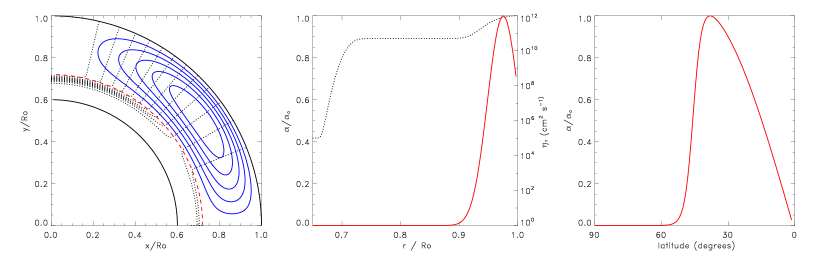
Figure 1: Profiles of the main ingredients of the solar dynamo. The left panel shows the contours of iso-rotation (dotted lines) together with the meridional flow streamlines (solid contours), the dashed line at $r$$=$$0.715R_{\odot}$ indicates the center of the overshoot region. The middle panel shows the radial variation of the BL $\alpha$ term (solid line) and the magnetic diffusivity, $\eta_{T}$ (dotted line). The values for $\alpha$ are normalized to its maximum value $\alpha_{0}$, and the values of $\eta_{T}$ are at the right axis. The right panel shows the latitudinal profile of the BL $\alpha$ term.

Both the contours of the iso-rotation and the streamlines of the meridional flow are shown in the left panel of Fig. 1. For all simulations presented below we consider a meridional flow amplitude of $u_{0}/2$$=$$15$ m s^-1 and a depth of penetration $r_{p}$$=$$0.7R_{\odot}$. Note that $u_{0}/2$ gives the maximum flow-speed (i.e. 15 ${\rm m}\,{\rm s}^{-1}$) for a maximum $u_{0}=30\,{\rm m}\,{\rm s}^{-1}$ for the mathematical prescription of meridional circulation we are using. In this calculation, we consider that the tachocline is centered at $0.7R_{\odot}$ with a thickness $\omega$$=$$0.03R_{\odot}$ (see e. g. Guerrero & de Gouveia Dal Pino (2007a)).

2.2 Diffusivity profile

The magnetic diffusivity is another important ingredient in dynamo models, but we know very little about the amplitude and profile of this ingredient in the solar interior. At the surface, it should be of the same order as the supergranular diffusion, and at the radiative layer and beneath it should attain molecular values. However we do not have a good idea what value it should have in the bulk of the convection zone. Recently the turbulent diffusivity for large-scale magnetic fields has been estimated using the so-called test field method for isotropic turbulence (Sur, Brandenburg & Subramanian, 2008) and convection (Käpylä et al., 2009). According to these studies, the turbulent diffusion is of the same order of magnitude as the first order smoothing estimate. This is in agreement with mixing length arguments for the kinematic regime in the range of currently accessible Reynolds number.

While the calculation by Käpylä et al. (2009) is a substantial advance and the best available today, given the limitation of computer powers, it is still far from solar-like conditions in terms of Reynolds number and the stratification. Inclusion of more realistic solar conditions as well as the ${\bf j}\times{\bf B}$ back-reaction that allows the formation of intense flux tubes may reduce the effective diffusivity in the bulk of convection zone. Furthermore, previous flux-transport dynamo studies have shown that the magnetic diffusivity is required to be one order of magnitude lower in the convection zone than at the surface in order for the dynamo to operate in the advection-dominated regime. So, in this work we use a diffusivity profile that has been used previously in several works (e.g., Dikpati et al. (2002); Guerrero & de Gouveia Dal Pino (2007a)), as follows:

$$\eta_{T}(r)=\eta_{rz}+\frac{\eta_{cz}}{2}\left[1+erf\left(\frac{r-r_{c}}{d_{1}}\right)\right]+\frac{\eta_{s}}{2}\left[1+erf\left(\frac{r-r_{c1}}{d_{2}}\right)\right]\quad,$$ (4)

where $\eta_{rz}$$=$$10^{5}$ cm² s^-1, $\eta_{cz}$$=$$5\times 10^{10}$ cm² s^-1 and $\eta_{s}$$=$$10^{12}$ cm² s^-1 correspond to the values of the diffusivity at the radiative, convective and near-surface layers, respectively. The transition from the radiative to the convective layers is located at $r_{rc}$$=$$0.715R_{\odot}$ (the overshoot interface), with $d_{1}$$=$$0.015R_{\odot}$, and the transition from the turbulent convective zone to the (sub-surface) supergranular diffusion layer is at $r_{rc}$$=$$0.96R_{\odot}$, with $d_{1}$$=$$0.03R_{\odot}$ (see the dotted line in the middle panel of Fig. 1).

2.3 Formulation of dynamo equations with $\eta$-quenching

As mentioned earlier, the main goal of this work is to study the quenching of the turbulent diffusivity due to the presence of strong magnetic fields. For this aim we will assume that it will affect only the toroidal fields, and replace $\eta_{T}$ in the equation for $B$ (eq. 3) by $\eta$:

$$\eta=\frac{\eta_{T}}{1+(B/B_{q})^{2}}\quad,$$ (5)

which is the same algebraic form for the $\eta$-quenching used by Gilman & Rempel (2005). In the equation above, $B_{q}$ is the value of the magnetic field at which $\eta_{T}$ begins to be quenched. In principle, the poloidal fields also could contribute to the diffusivity quenching. However, here we focus only on the influence of toroidal fields in the saturation mechanism of the the turbulent diffusivity for two reasons: (1) in most of the $\alpha$-$\Omega$ solar dynamos, the dynamo-generated toroidal fields are about a thousand times stronger than the poloidal fields; (2) the amplitude of poloidal fields generated in a Babcock-Leighton flux-transport dynamo is of the order of a few hundred Gauss, much below the value of the lowest quenching field strength selected for the study in this paper. In a more realistic situation, the diffusivity is a tensor and its quenching is bound to have some effect due to the presence of poloidal fields also, and must be explored in future.

Before we re-derive the dynamo equations with the inclusion of $\eta$-quenching, we briefly discuss the issue regarding the choice of $\eta$-quenching formula. Analytical studies considering 3D turbulence often yield a quenching formula proportional to $|B|$ rather than $B^{2}$ (Kitchatinov, Pipin & Rüdiger, 1994; Rogachevskii & Kleeorin, 2001).

In turbulent forced MHD simulations, Yousef et al. (2003) found that the suppression of the magnetic diffusivity follows the form: $\eta$$\simeq$$\eta_{T0}/(1+a({{\bf B}/B_{eq}})^{2})$, where the value of $a$ depends on the geometry of the initial magnetic field (i.e. whether it is helical or not). Käpylä and colleagues (see $http:\/\/arxiv.org\/abs\/0810.2298$) have also recently performed numerical simulation where turbulent diffusivity is quenched. However, their results are not able to make a clear conclusion about the functional form of quenching to be proportional to $|B|$ or $B^{2}$. In the present case, we will adopt a similar formulation, but with $B_{q}$ as a free parameter of the model. The results of Yousef et al. (2003) indicate that in the solar convection zone $\eta_{T}$ is quenched approximately as in eq. (5) for fiducial choices of the value of $B_{q}$.

We note that, with the quenching incorporated, $\eta$ is not only a function of $r$, but also depends on $B(r,\theta,t)$, and hence $\eta(r,\theta,t)$ is a function of $r$, $\theta$ and $t$. Due to the additional dependence of $\eta(r,\theta,t)$ on $\theta$ and $t$, the $\theta$ component of $\nabla\eta\times(\nabla\times B\hat{e}_{\phi})$ gives rise to two new terms in the induction equation.

Thus the Equation (3) becomes:

$$\frac{\partial B}{\partial t}+\frac{1}{r}\left[\frac{\partial}{\partial r}[ru_{r}B]+\frac{\partial}{\partial\theta}[u_{\theta}B]\right]=s({\bf B_{p}}\cdot\nabla)\Omega$$ (6)

$$-\left[\frac{\partial\eta}{\partial r}\left(\frac{\partial B}{\partial r}-\frac{B}{r}\right)+\frac{1}{r^{2}}\frac{\partial\eta}{\partial\theta}\left(B\cot\theta+\frac{\partial B}{\partial\theta}\right)\right]_{\phi}$$

$$+\eta\left(\nabla^{2}-\frac{1}{s^{2}}\right)B\quad,$$

2.4 Babcock-Leighton $\alpha$ effect

The source of poloidal fields (eq. 2) in a Babcock-Leighton dynamo is the decay of the tilted bipolar magnetic regions (BMR’s), which form a net surface dipole moment that drift towards the poles and eventually cause the reversal of the polar fields. The place where the magnetic flux tubes, which are responsible for the formation of the BMR’s, develop is uncertain, but due to various reasons we can assume that the flux tubes are formed at or below the base of the convection zone. There exists a vast literature on the topic of rising flux tube simulations that produce the tilt and emergence pattern at the solar surface which are in good agreement with observations (see, for example, D’Silva & Howard (1993); Fan, Fisher & McClymont (1994)). The combination of low magnetic diffusivity and helioseismically obtained differential rotation helps the amplification of toroidal fields there.

Furthermore, the rising flux tube simulations indicate that their eruption latitude and the tilt acquired during their buoyant rise through the convection zone fit best with surface observations if flux tubes with magnitudes between $5\times 10^{4}$ and $10^{5}$ G are produced at the bottom of the convection zone. .

Estimating the Babcock-Leighton $\alpha$-effect by computing the buoyant eruption of magnetic flux tubes followed by their decay is beyond the scope of this paper. So, in order to capture the properties of the BMR’s described above, we simply use the following Babcock-Leighton $\alpha$ effect profile (Dikpati et al., 2004):

$$S_{1}(r,\theta,B)=\alpha(r,\theta)f_{Q}(\overline{B_{r_{c}}})\overline{B_{r_{c}}}\quad.$$ (7)

This term is non-local in $B$ (see below), $\overline{B_{r_{c}}}$ being the radial average of $B$ between $r$$=$$0.7R_{\odot}$ and $r$$=$$0.72R_{\odot}$; this is a simple way to erupt toroidal magnetic flux from the bottom of the convection zone to the place where the $\alpha$-effect is operating. We incorporate the following radial and latitudinal dependence of the $\alpha$-effect:

$$\alpha(r,\theta) = \alpha_{0}\frac{1}{4}\left[1+\mathrm{erf}\left(\frac{r-r_{2}}{d_{2}}\right)\right]\left[1-\mathrm{erf}\left(\frac{r-r_{3}}{d_{3}}\right)\right]$$

$$\times \sin\theta\cos\theta\left[\frac{1}{1+e^{\gamma_{1}\left(\pi/4-\theta\right)}}\right]\quad,$$

where $r_{2}$$=$$0.95R_{\odot}$, $r_{3}$$=$$R_{\odot}$, $d_{2}$$=$$d_{3}$$=$$0.01R_{\odot}$, and $\gamma_{1}$$=$$30$. The amplitude of the poloidal source is determined by $\alpha_{0}$, for which we assume a fixed value of $50$ cm s^-1 for the first set of simulations below (from now onwards we will explicitly quote the value of $\alpha_{0}$ only when we are using a value different from this). As can be seen in Fig. 1, the $\alpha$-effect is distributed mainly at the low latitudes peaking around $45^{\circ}$; it is also concentrated above $0.95R_{\odot}$ since it is expected that the main poloidal field component is formed at the sunspot latitudes near the surface (Wang et al., 1989; Wang & Sheeley Jr, 1991).

The quenching of the poloidal source term (the second term of eq. 7) is given by:

$$f_{Q}(B)=\left(1+\left[\frac{\overline{B_{r_{c}}}(\theta)}{B_{0}}\right]^{2}\right)^{-1}\quad.$$ (9)

This term has the same algebraic form as the $\alpha$-quenching term used in turbulent mean field dynamo models. Its function here is to saturate the growing of the poloidal fields when the toroidal field at the base of the convection zone is around $B_{0}$$=$$10^{4}$ G. Thus the model will produce toroidal magnetic fields in the expected range, as explained above. The amount of poloidal field that will be produced from this toroidal field is determined by $\alpha_{0}$. We note that this is not the unique way of capturing the physics of buoyantly erupted flux tubes. Nandy & Choudhuri (2001) have replaced this non-local quenching term by a different buoyancy mechanism term parameterized from simulations of flux tubes.

Although the equations (5) and (9) have the same functional form, they operate in opposite ways. We will discuss that in detail in §4. On the one hand, smaller values of $B_{q}$ in eq. (5) will produce lower values of $\eta$ which will, in turn, help to increase the amplitude of the toroidal component, $B$. On the other hand, lower values of $B_{0}$ in eq. (9) will limit the growth of $B$ up to values around $B_{0}$. Both these terms are the sources of non-linearity in the model.

3 SOLUTION METHOD, BOUNDARY AND INITIAL CONDITIONS

We solve equations (2), (3) and (5) for $A$ and $B$ and $\eta$, with the coordinates $r$ and $\theta$ covering the spatial range $0.6R_{\odot}$$\leq$$r$$\leq$$R_{\odot}$ and $0$$\leq$$\theta$$\leq$$\pi/2$, which spans from the outer most part of the radiative zone, through the overshoot layer (where the tachocline is located) and the entire convection zone, up to the surface, in the northern hemisphere. We have used a second order finite difference scheme for the spatial discretization; the Lax-Wendroff method for the first order derivatives, and centered finite difference for the second order derivatives. The temporal evolution is solved with the ADI semi-implicit method (see Guerrero & Mũnoz (2004); Dikpati & Charbonneau (1999), for details). In eq. (5), the dependence of $\eta$ with time is implicit, thus we update the value of $\eta$ each half-time step with the previous values of $B$ and then we calculate the derivatives of $\eta$ and use these values to solve the equation for $B$.

The boundary conditions are: $A=0$ and $B=0$ at the north pole ($\theta=0$); and at the equator $B=0$, but $A$ is coupled with the southern hemisphere in such a way as to ensure antisymmetric magnetic fields about the equator, so we demand ${\partial\over\partial\theta}\left(r\sin\theta A\right)=0$. At the bottom radial boundary we use $A={\partial\over\partial r}(rB)=0$, and finally, at the upper radial boundary $r=R_{\odot}$, we consider a potential field boundary, i.e., $B=0$ and $A$ coupled to an external vacuum field $(\nabla^{2}+1/s^{2})A=0$. A complete description of the boundary conditions and their numerical implementation can be found in Dikpati & Choudhuri (1994); Dikpati & Charbonneau (1999).

Since our intention is to explore how the $\eta$-quenching affects a magnetic field that is well organized both in space and time, a plausible choice for an initial condition for the simulation is to start with a fully relaxed solution of the same dynamo without $\eta$-quenching. So we first obtain a fully converged solution by initializing the system with $A=\sin\theta/r^{2}$ if $r\geq 0.715$, $A=0$ otherwise, and $B=0$, and allow it to evolve until $10^{4}$ yr with the $\eta$-quenching in the Equation (6) turned off.

Figure 2 shows the time-latitude, butterfly diagram for the last $60$ years of evolution of our reference simulation. It shows the gray scale (color) contours of the radially averaged toroidal magnetic field $\overline{B_{r_{c}}}$ (in log-scale) with values above $12$ kG, together with the contours of the radial field $B_{r}$ at the surface. It can be seen that the maximum amplitudes of the toroidal field are located below $45^{\circ}$, and satisfy the $\pi/2$ phase-lag observed with respect to the radial field. The maximum value of the toroidal magnetic field $\overline{B_{r_{c}}}$ is $\sim 22.9$ kG, the maximum value of the radial field is $86.6$ G, and the period of the entire cycle is $21.2$ yr.

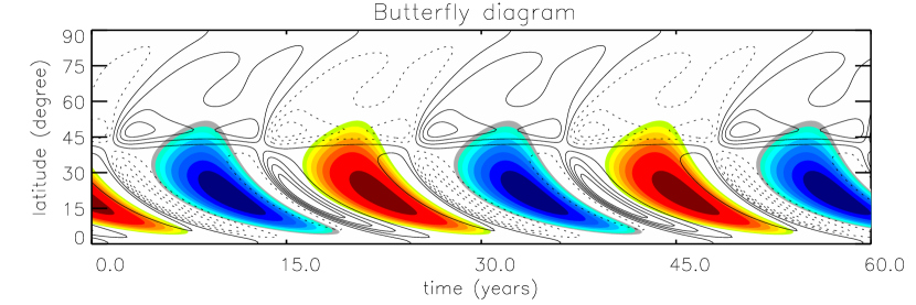
Figure 2: Butterfly diagram for the relaxed solution of the reference model. The dark (blue) contours represent positive toroidal fields and the light (red) contours represent the negative toroidal fields. The plotted values correspond to a radial average between $0.7R_{\odot}$ and $0.72R_{\odot}$. Only contours for fields above $1.2\times 10^{4}$ G are plotted. The continuous and dashed lines represent the positive and negative radial fields at the surface, respectively.

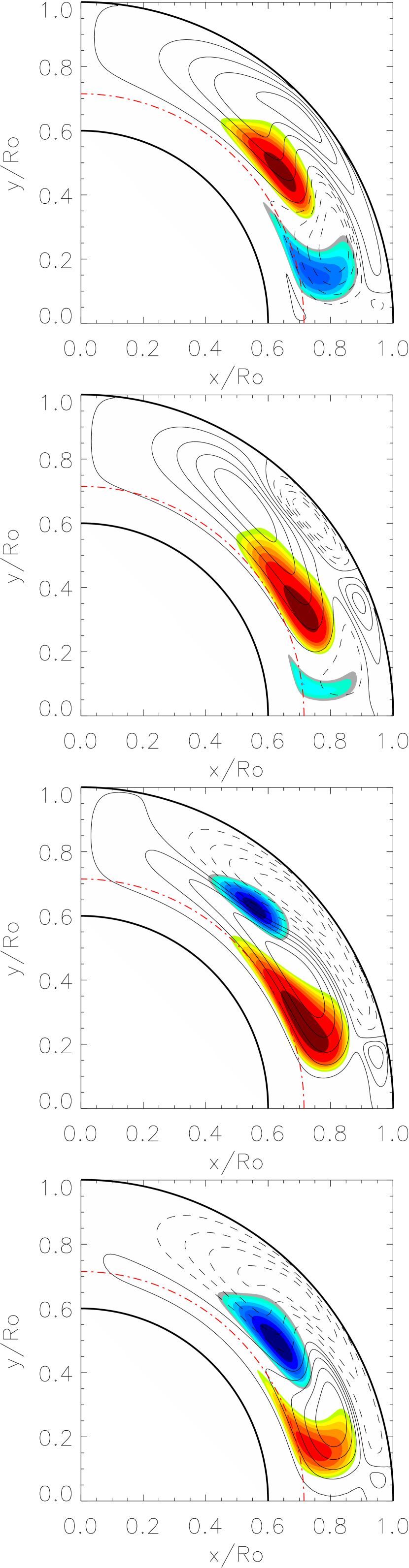
Figure 3: Snapshots of the relaxed solution of our reference model at $0$, $T/8$, $T/4$ and $T/2$, where T is the full period of the cycle. The gray scale (color) contours follow the same description as in Fig. 2, but in this case the line contours correspond to the total poloidal field.

The four frames of Fig 3 (a-d) show the same temporal evolution in the meridional cut. We see that the strongest toroidal fields begin to form at mid-latitudes inside the convection zone ($r$$\sim$$0.8R_{\odot}$). The toroidal field penetrates slightly in the overshoot layer only at lower latitudes, but it is not substantially amplified there by the radial shear. This happens due to two reasons: first, since the meridional flow is not allowed in this model to go deep inside the overshoot layer, not enough poloidal fields (which are actually the source for the toroidal fields) can reach the radial shear layer; second, the radial component of the poloidal field is much weaker there than the latitudinal component (Guerrero & de Gouveia Dal Pino, 2007a). Fig 3 also reveals that the positive and negative poloidal magnetic fields (continuous and dashed lines, respectively) are produced at mid-latitudes at the surface and then migrate poleward following the plasma flow.

We use the converged solution without the $\eta$-quenching shown in Figures 2 and 3 as our initial ($t=0$) configuration for our simulations with $\eta$-quenching and run the model for 200 years more. In §4, we present our simulation results with $\eta$-quenching.

4 Results

4.1 The effect of $\alpha$-quenching term in Babcock-Leighton dynamos

Generally $\alpha$-quenching is applied in most of the large-scale, mean-field dynamo models and the basic results are known. In a kinematic dynamo, the maximum value that the toroidal field can reach depends on the amount of poloidal field being generated by the Babcock-Leighton $\alpha$-effect, and the later depends on the values of $\alpha_{0}$ and $B_{0}$ in Equations (2.4) and (9). In order to explore the influence of $\alpha$-quenching in more detail and to compare this influence with that obtained by implementing the $\eta$-quenching, we study how the maximum toroidal fields produced at different latitudes vary with the quenching field strength. The value of $\alpha_{0}$ defines the non-dimensional number $C_{\alpha}$$=$$\alpha_{0}R_{\odot}/\eta_{cz}$$=$$70$ for $\alpha_{0}$$=$$50$ cm s^-1 and $\eta_{cz}$$=$$5\times 10^{10}$ cm² s^-1, this value remains constant during all the simulations shown below. This guarantees that the dynamo efficiency $C_{\Omega}C_{\alpha}$ is always the same. Then, we change the value of $B_{0}$ in eq. (9) between $5\times 10^{2}$ G and $5\times 10^{5}$ G and measure the maximum value that the toroidal field reaches at the numerical domain during one-half period. Intuitively we expect that the maximum value of $B_{max}$ should be larger for larger $B_{0}$.

Fig. 4 presents $B_{max}$ as function of $B_{0}$ for two different radii $r$$=$$0.7R_{\odot}$ and $r$$=$$0.8R_{\odot}$, and three different latitudes, $10^{\circ}$ (continuous line), $45^{\circ}$ (dashed line) and $80^{\circ}$ (dotted line). Figure 4 immediately reveals that maximum toroidal fields generated at different latitudes and different depths vary near linearly with the quenching field strength; the higher the quenching field strength the higher the dynamo-generated toroidal field. This means that the nonlinearity due to $\alpha$-quenching is so weak even up to a quenching field strength of $10^{5}$ Gauss that the dynamo behaves virtually as if it is operating in the linear regime.

We also see that for lower latitudes ($<45^{\circ}$), the maximum toroidal field is of the same order both in the convection zone ($r$$=$$0.8R_{\odot}$) and at the tachocline ($r$$=$$0.7R_{\odot}$). This is because the largest toroidal fields in a Babcock-Leighton flux-transport dynamo are produced mainly by the latitudinal shear working on the latitudinal poloidal fields rather than by the action of tachocline radial shear on radial fields. This reinforces the result obtained previously by some authors (Rempel, 2006; Dikpati, de Toma & Gilman, 2006; Guerrero & de Gouveia Dal Pino, 2007a). With no advective transport below the base of the convection zone, very little poloidal field diffuses down there, and due to the thinness of the tachocline, an even smaller radial component of those poloidal fields is available to be sheared there. However, the situation can be different if the magnetic fields can be transported downwards by overshooting or magnetic pumping at the lower latitudes and then acquire further amplification at the radial shear layer (Guerrero & de Gouveia Dal Pino, 2008).

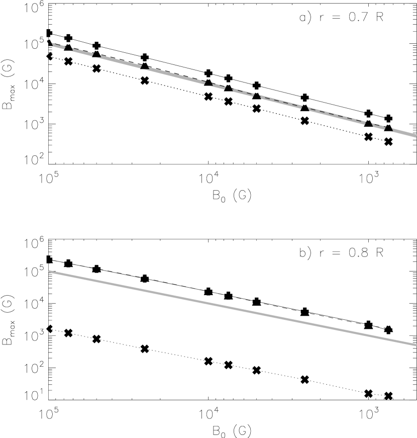
Figure 4: Maximum toroidal magnetic field as function of $B_{0}$ at $r$$=$$0.7R_{\odot}$ and $r$$=$$0.8R_{\odot}$ (see the $\alpha$ quenching function, eq. (9)) for three different latitudes, $10^{\circ}$ (continuous line, cross symbol), $45^{\circ}$ (dashed line, triangle symbol) and $80^{\circ}$ (dotted line, $X$ symbol). In the bottom panel, the continuous and dashed lines are almost coincident. In each panel, a $B_{\rm max}=B_{0}$ curve has been superimposed to show the linear proportionality of maximum toroidal fields produced by a certain $\alpha$-quenching field strength.

4.2 The effects of $\eta$-quenching in magnetic field evolution

It has already been noted in the context of one-dimensional $\alpha\Omega$ dynamo, two-dimensional $\alpha^{2}\Omega$ dynamo and interface dynamo that, the quenching of the magnetic diffusivity due to the back-reaction of magnetic fields is a possible mechanism for further field amplification. In this subsection, we first explore in detail the evolution of magnetic fields in a diffusively-quenched Babcock-Leighton flux-transport dynamo, starting from the 2D reference-state solution described in §3. Subsequently we will also present the quantitative estimation of field amplification and the change in cycle period due to $\eta$-quenching.

In the case of the $\alpha$-quenching study, we ran our simulation for $5\times 10^{2}{\rm G}\leq B_{0}\leq 5\times 10^{5}{\rm G}$. We consider same range for $B_{q}$ for the $\eta$-quenching study: $5\times 10^{2}{\rm G}\leq B_{q}\leq 5\times 10^{5}{\rm G}$, and keep all the other parameters the same as in the reference model described in §3. Using a fully converged solution of the reference model as the initial condition, we switched on the $\eta$-quenching and ran the simulation for $200$ years. At this time, the system reaches a new steady state with cyclic variations of $A$, $B$ and $\eta$.

It is not surprising that, the smaller the $B_{q}$, the faster the $\eta_{T}$ is quenched, leading to a significant increase in toroidal field. Figures 5 and 6 show the temporal evolution of both, the toroidal and poloidal fields in the pole-to-equator meridional-cut for four successive times within half a cycle (left panels) for two different representative values of $B_{q}$ ($10^{4}$ G and $10^{3}$ G, respectively). These are the solutions after 200 years’ evolution. Right panel shows the change of $\eta$ due to the quenching action, for two different latitudes, $10^{\circ}$ (solid line) and $45^{\circ}$ (dashed line). The non-quenched profile has been plotted also for comparison (red dotted line).

The common features in both cases (see Figures 5 and 6) are that the model exhibits a decrease in the diffusivity at the places where the toroidal field acquires considerable amplitude. This suppression can be as large as three orders of magnitude, as we see in Figure 6 for $B_{q}=10^{3}$ G, but this suppression of $\eta$ is not uniform – neither along the radial direction nor in latitude. Comparing the left and right panels in each of Figures 5 and 6, we see that the peaks and valleys are anti-correlated with the spatial distribution of the toroidal field amplitudes. Since we are presenting here the converged solution, this change in $\eta$ repeats in successive cycles.

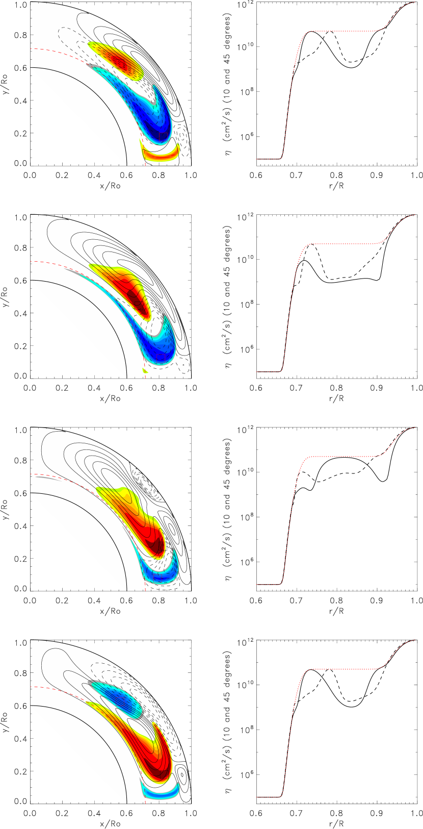
Figure 5: Left panel: Snapshots for 4 different times within a half period of the relaxed model for $B_{q}$$=$$10^{4}$ G. Right panel: Turbulent diffusivity without quenching (red dotted line), for $10^{\circ}$ (continuous black line) and $45^{\circ}$ (dashed blue line).

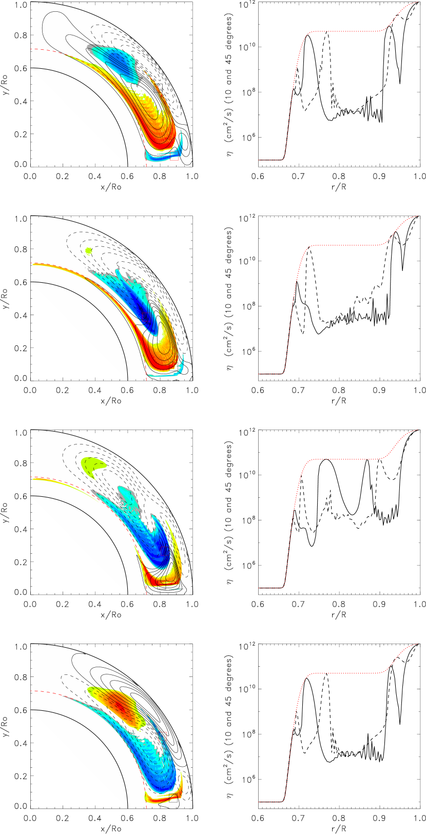
Figure 6: The same as in Fig. 5, but for $B_{q}$$=$$10^{3}$ G.

In both cases, strong gradients in diffusivity in latitude as well as in depth occur, leading to the more efficient field amplification in those regions and hence, the formation of small regions of concentrated toroidal magnetic fields. Comparing Figures 5 and 6 with Figure 3, we can see the enhancement in magnetic fields even in places where a run without quenching does not exhibit strong toroidal fields.

It is not difficult to understand why the diffusivity quenching leads to small regions of flux concentrations in the computation domain. The average diffusion time of the fields at each portion of the domain where $\eta$ is strongly suppressed is larger than the neighbouring domains where the quenching is less effective. The lifetime of the toroidal fields is several years larger there than in the regions where the quenching is not as effective. Thus the former can undergo a prolonged amplification by the $\nabla\Omega$ terms and can reach larger values than the neighbouring regions that have larger $\eta$ .

An interesting feature we note in Figure 6 is the formation of small scale magnetic patterns at the overshoot tachocline (see in the left panels). This is associated with a variation in $\eta$ in finer spatial scale compared to what we see in Figure 5 as a function of depth. This is a consequence of the non-linear coupling between $B_{q}$ and $\eta$. The smaller the $B_{q}$, the narrower the $\eta$ profile, and the more segregation of the magnetic fields is produced . Due to large suppression in $\eta$ at the overshoot tachocline regions, the spot-producing toroidal flux remains more frozen there, particularly in the case of Figure 6. In the meantime, two competing processes are going on – the prolonged shearing by the differential rotation, and the equatorward advection due to meridional flow. Since this advection must work against the diffusion of the fields, we can think of it as “dragging” or “pulling” the fields along, at some net speed that is smaller than the meridional flow there. If the equatorward advective drag partially wins at certain portions of these fields, those portions get torn out from the large-scale part of the fields, and locally reconnect. This happens predominantly on the equatorial side of the large-scale fields, and so more and more fragmentation of field takes place, leading to formation of small-scale structures.

4.3 Influence of $\eta$-quenching on field amplification

In order to quantify how effective the $\eta$-quenching is in producing strong toroidal fields, we have plotted in Fig. 7 the maximum value of the dynamo-generated toroidal field as a function of $B_{q}$. As in Fig. 4, we show the results at three different latitudes: $10^{\circ}$ (solid line), $45^{\circ}$ (dashed line) and $80^{\circ}$ (dotted line), for two different radii, namely for $0.7R_{\odot}$, the center of the tachocline, and $0.8R_{\odot}$, the lower convection zone.

At the tachocline (upper panel of Fig. 7), the curves show an interesting behaviour: at latitudes close to the poles (dotted line), the toroidal field increases with decreasing $B_{q}$ (i.e., with increasing quenching). The amplification factor could be up to $\sim 2.5$. We can understand this, because the poloidal fields carried down to the tachocline by the meridional flow, undergo prolonged shearing by the strong radial differential rotation there. However, we obtain an apparently counter-intuitive result that for lower latitudes (solid lines), there is a decrease of $B$ with the increased quenching in $\eta$ (decrease in $B_{q}$). We see a little decrease of $B$ at mid-latitudes also as $B_{q}$ decreases, but the effect is not so pronounced, and appears only for very efficient quenching factors. For the fields at $10^{\circ}$, the factor of decrease could be as large as $\sim 2.5$.

At the center of the convection zone (bottom panel of Fig. 7), the results are different; the magnetic fields for both low and mid-latitudes have the same increase, by a factor as large as $\sim 2$ with respect to the case with no quenching. With $B_{q}=5\times 10^{3}$ G the toroidal fields can reach values above $10^{5}$G. In the middle of the convection zone there is no radial shear. It is the latitudinal shear that works on the poloidal fields, so we see similar amplification for mid-latitude and low-latitude fields. If the flux tubes formed from these strong toroidal fields produced at the middle of the convection zone due to strong $\eta$-quenching, rise to the surface, their orientation may not agree with Joy’s law. So we do not know whether such a strong $\eta$-quenching is working in reality, or some other processes are inhibiting the formation of flux tubes in the middle of the convection zone.

Figure 7: Maximum toroidal magnetic field as function of $B_{q}$ (see the eq. (5) for three different latitudes, $10^{\circ}$ (continuous line, cross symbol), $45^{\circ}$ (dashed line, triangle symbol) and $80^{\circ}$ (dotted line, $X$ symbol). At the bottom panel, only the results for $10^{\circ}$ and $45^{\circ}$ are shown, the maximum values of $B$ for $80^{\circ}$ are smaller than $10^{4}$ G.

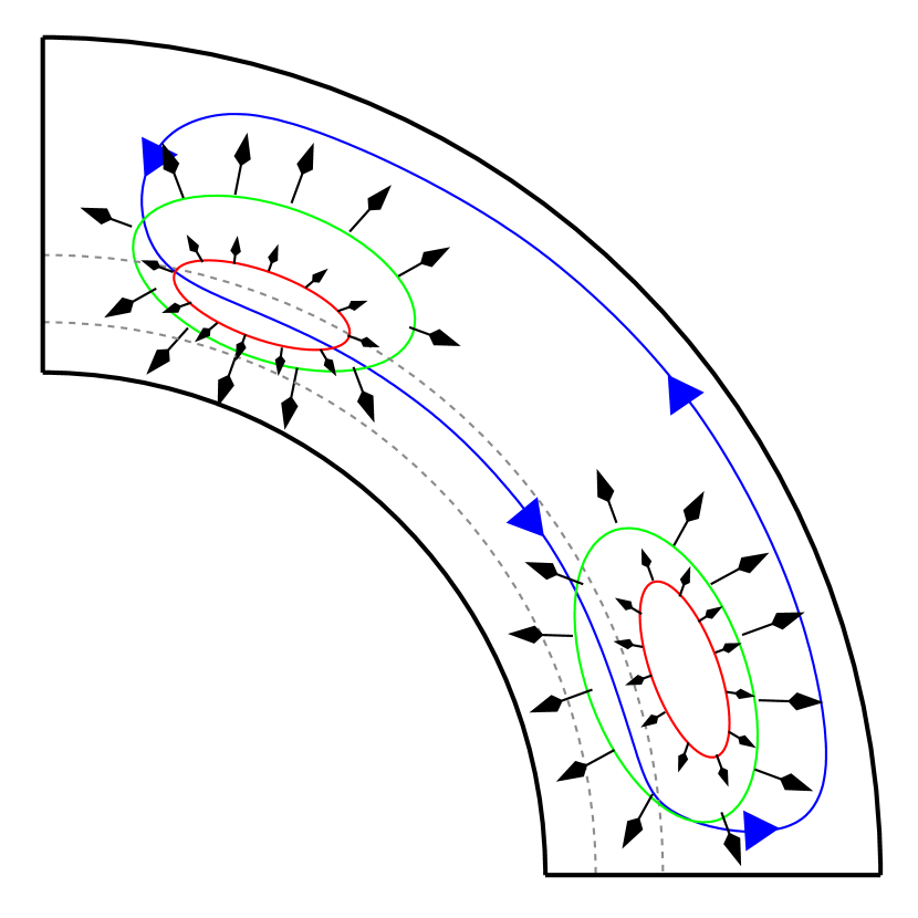
Figure 8: Schematic diagram shows how, with the help of downward advective transport, the high-latitude toroidal fields (cross section of which is represented by the red loop, direction being perpendicular to the plane of the paper) can access the shear layer (within gray doted lines) is more efficiently amplified when there is strong $\eta$-quenching. This can be compared to the toroidal fields without $\eta$-quenching (cross-section is represented by the green loop, direction being perpendicular to that loop), which diffuse more efficiently. By contrast, the upwelling flow at low-latitudes makes the toroidal fields stay away from the shear layer when diffusivity is more suppressed (see the low-latitude red-loop).

The contrasting feature of the field amplification at high and low latitudes in the tachocline (see the dotted line and solid line in the upper panel of Figure 7) occurs, respectively, due to the difference in advective transport at high and low latitudes. If it would have been due to the suppression of the diffusivity and hence a prolonged shearing effect, we would have expected the increase in field amplitude in all latitudes. Clearly the directional transport plays some role here. We can understand this by using the schematic diagram shown in Figure 8. The advective transport being downward at high-latitudes, the poloidal fields there can reach the shear layer, for both cases when there is no $\eta$-quenching and when there is strong $\eta$-quenching. But in the latter case, the toroidal fields, originated from the sheared poloidal fields there, undergo less diffusion and stay at the tachocline shear layer for longer time than in the former case. The high-latitude toroidal fields (which are normal to the red loop in the figure) undergo further amplification due to local feeding by new toroidal field lines that are created by shear due to the strong tachocline differential rotation, compared to the case without $\eta$-quenching where the toroidal field undergoes more diffusion (see the high-latitude green loop which represents a section normal to a bunch of toroidal field lines without $\eta-$-quenching). As a consequence, with the increase in the $\eta$-quenching, there is a systematic increase in the high-latitude toroidal field amplitude.

On the other hand, the upwelling flow near the equator pushes the low-latitude poloidal fields upward, away from the shear layer, making it difficult to create toroidal fields at such latitudes. However a question arises here: the low-latitude poloidal fields are advected upward always, no matter whether the $\eta$-quenching is present or not, but why do the low-latitude toroidal fields decrease with the increased $\eta$-quenching (with decreasing $B_{q}$), instead of being independent of $B_{q}$? Again we take the help of the schematic diagram in Figure 8 to explain this feature. This happens due to the combination of decrease in diffusivity and upward transport. In spite of the fact that the meridional flow at low latitudes always takes the poloidal fields away from the radial shear layer, there is a small amount of toroidal field being produced there and another amount produced at the convection zone due to latitudinal shearing. Given that the only mechanism that is able to transport the toroidal field downwards, at low latitudes, is the diffusive transport, in the case without $\eta$-quenching (green loop), the toroidal field produced in the convection zone expands and reaches a portion of the tachocline. There, it encounters the existing amount of toroidal field and thus, increases its magnitude. However, in the case with $\eta$-quenching, the toroidal field produced in the convective zone remains confined to a small region (red loop) and the toroidal field at the tachocline is not effectively increased. Hence the decrease in field amplification at low latitudes happens with increased $\eta$-quenching.

4.4 Influence of $\eta$-quenching in butterfly diagram and cycle period

The increase in high-latitude toroidal fields and decrease in low latitude toroidal fields in the tachocline regions, with smaller $B_{q}$, will influence the butterfly diagram accordingly. We recall again that the contours of the toroidal field that appear in the diagrams are computed from the radial average over the overshoot region.

Figure 9 shows several butterfly diagrams for different values of $B_{q}$. It can be seen how the butterfly wings, that are predominantly concentrated within latitudes $\leq 45^{\circ}$ when $B_{q}$ is large (less quenching), move to higher and higher latitudes as $B_{q}$ decreases (more quenching). This happens for the same reason that low-latitude fields at the tachocline decrease whereas the high-latitude fields increase with enhanced $\eta$-quenching. If a very large suppression in the $\eta$ occurs, the butterfly diagram produced from this model will not be in accordance with observations. The obvious question arises whether we can estimate how much $\eta$-quenching should be expected. Brandenburg (2001) showed in a direct numerical simulation of dynamos that the saturation level of the magnetic field is often close to the equipartition field strength given by, $B_{e}q=\sqrt{\mu_{0}\,\rho\,u^{2}}$ in MKS unit, or $=\sqrt{1/2\,\rho\,u^{2}}$ in CGS unit, where $u$ is the rms value of the turbulent velocity, $\mu_{0}$ is the conversion factor between CGS and MKS unit and $\rho$ is the plasma density. With approximate values of the turbulent velocity of 5000 ${\rm cm}\,{\rm s^{-1}}$ at the base of the convection zone and density of 0.2 gm/cc, the equipartition magnetic field comes out to be approximately $10^{4}$ Gauss. Assuming that the back-reaction of the magnetic fields to quench the $\eta$ will not start until the equpartition field strength is reached, the butterfly diagram will not depart much from observations. By contrast, in the present calculations large departures from the observed butterfly diagram occur for $B_{q}\lesssim 500$Gauss (see Fig. 9d), but according to the above arguments, $\eta$-quenching should not occur for fields so far below equipartition.

Note also that in the bottom panel of Fig. 9 the toroidal field shows some small-scale structures, as we saw in the toroidal field patterns in Figure 6. We repeat here that the primary reason for the formation of these fragmented, small-scale structures is the competition between the two transport effects; the fields tend to remain more frozen due to the lowering in the diffusivity while the equatorward advective drag is pulling them, eventually causing their fragmentation. In order to check whether these are merely the numerical effects due to resolution problem, we have performed three experiments, namely doubling the resolution (experiment #1), reducing the advective speed to half of the value used in the present paper (experiment #2) and doubling the advective speed (experiment #3). The results (figures not included) indicate that the fragmented, small-scale structures do not go away with the increased resolution; nor do they go away when the meridional flow-speed is reduced, but those structures are almost gone when the flow-speed is doubled, because advection wins the competition in that case. Perhaps a minor contribution into those small-scale structures comes from the numerical effect due to model diffusivity reaching the limit of grid-diffusion, but our experiment #3 confirms our physical explanation that the formation of those small-scale structures are the consequences of the two aforementioned competing processes.

With smaller values of $B_{q}$, it is possible to reach larger magnetic fields; however the system does not reach a steady state.

The changes in the butterfly patterns indicate that these diagrams remain consistent with observations up to a certain increase in the $\eta$-quenching, but the influence of an enhanced $\eta$-quenching is to make the butterfly-diagrams depart further from the observations. The shift in the butterfly wings towards higher latitudes could cause another problem in the dynamo model, namely loss in the coupling between the two hemispheres across the equator and hence, a shift to the quadrupole parity in the solution when solved in a full spherical shell. In that case, to restore the observed dipolar parity of the large-scale solar magnetic fields, the help of additional downward transport using turbulent pumping may be required (Guerrero & de Gouveia Dal Pino 2008). We leave those studies for the future.

In Fig. 9 we also see an increase in the dynamo cycle period with increasing $\eta$-quenching, i.e. with decreasing $B_{q}$. The number of butterfly wings produced in $60$ yr decreases. Figure 10 shows a plot of dynamo cycle period as function of $B_{q}$, and the decrease in cycle period with increased $\eta$-quenching is very clear. This happens due to the competition between the flux-freezing effect by the smaller diffusion and advective drag due to meridional flow. The suppression in $\eta$ due to quenching works against the advective transport of flux.

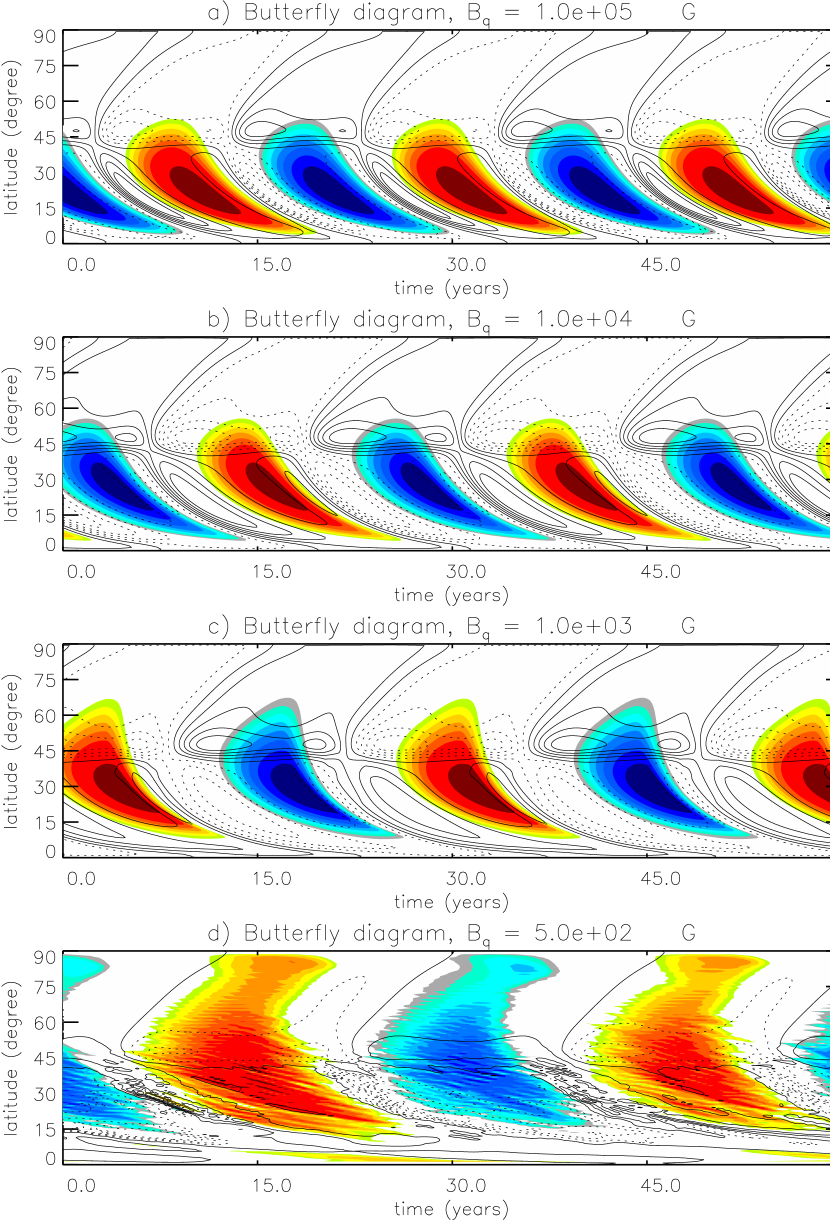
Figure 9: Butterfly diagrams for different values of $B_{q}$. Top: $B_{q}$$=$$10^{5}$ G; second from top: $B_{q}$$=$$10^{4}$ G; third from top: $B_{q}$$=$$10^{3}$ and bottom: $B_{q}$$=$$5\times 10^{2}$ G.

4.5 Advection-dominated versus diffusion-dominated dynamos

In Babcock-Leighton dynamo models, the meridional flow is the conveyor belt that carries the magnetic field, both at the surface in order to produce a new poloidal field, and at the bottom of the convection zone where it transports the toroidal fields in the direction of the equator in such a way that this flow dominates over other parameters in setting the period of the cycle (Dikpati & Charbonneau, 1999). But for this process to occur the advective term in eq. 1 must dominate the diffusive term in determining the time-scale of the system. Thus this class of models require values of $\eta_{cz}$$\lesssim$$2\times 10^{11}$ cm² s^-1. However, the values inferred from the mixing length theory at the surface are one to two orders of magnitude larger than the values considered in the bulk of the convection zone in the advection-dominated flux-transport dynamo models. To our knowledge, until now there is no accurate estimation of the magnetic diffusivity at the convection zone and beneath. This limitation have recently led to criticisms to the flux-transport scenario (see more about this discussion in Charbonneau (2007); Yousef et al. (2003)).

In previous sections, we have described the action of the $\eta$-quenching in a Babcock-Leighton dynamo and found that, depending on the quenching parameter $B_{q}$, the diffusivity can be locally suppressed by up to three orders of magnitude and this effect can also increase the cycle period (Figure 10). This is an indication that the average radial value of $\eta_{cz}$ is also being suppressed. One question arises here: will diffusion-dominated dynamos, which in general produce much faster cycles, change to advection-dominated dynamos due to the suppression of $\eta$ by quenching mechanism, and produce a cycle period similar to the observed sunspot cycle?

Figure 10: Half-cycle period as function of $B_{q}$.

Figure 11: Half-cycle period as function of $\eta_{cz}$ for $B_{q}$$=$$10^{3}$ G (triangle symbol) and $B_{q}$$=$$10^{4}$ G (cross symbol).

We have performed simulations to try to answer this question. We have increased progressively the diffusivity from $5\times 10^{10}$ cm² s^-1 (the value employed in the previous calculations) to the largest allowed value, namely $5\times 10^{11}$ cm² s^-1, for which we obtain an oscillatory solution (not decaying due to large diffusivity). The latter case is the diffusion-dominated regime, and the cycle period is small, determined by the diffusivity values. We then performed the same numerical experiments as before by switching on the $\eta$-quenching, for the two representative values of $B_{q}$, $10^{3}$ and $10^{4}$ G and maintained the constant dynamo efficiency defined by $C_{\Omega}C_{\alpha}$, for all the simulations. We note that keeping $C_{\Omega}C_{\alpha}=\alpha_{0}\Omega_{eq}R^{3}/\eta_{cz}^{2}=cte$ implies a change in $\alpha_{0}$ as $\eta_{cz}$ changes (see the Table 1 for the values used for $\alpha_{0}$ for each simulation, as well as the maximum values for the average toroidal field at the base of the convection zone, $\overline{B_{r_{c}}}$, and the radial field, $B_{r}$, at the surface).

In Figure 11, we present the dynamo cycle period as function of magnetic diffusivity for the two cases, with $B_{q}=10^{4}$ G (pluses) and $B_{q}=10^{3}$ G (triangles). The models with $B_{q}$$=$$10^{4}$ G (plus symbols) present two different regimes for the slope of the curve of the period versus $\eta_{cz}$. For values of $\eta_{cz}$$\leq$ $10^{11}$ cm² s^-1, the cycle period does not vary much with the value of $\eta$; it is primarily determined by the meridional flow speed. For $\eta_{cz}$$>$$10^{11}$ cm² s^-1, the cycle period varies more rapidly with $\eta_{cz}$, indicating that the models are operating in the the diffusion-dominated regime.

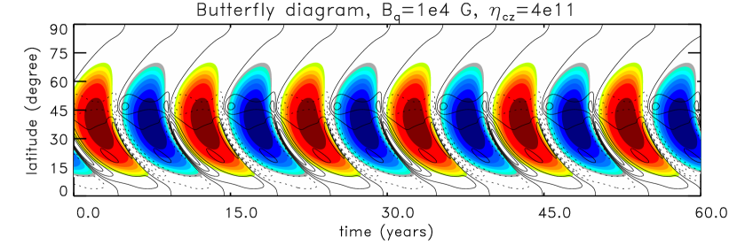
Figure 12: Butterfly diagram for the model with $B_{q}$$=$$10^{4}$ G and $\eta_{cz}$$=$$4\times 10^{11}$ cm² s^-1.

For the case of $B_{q}$$=$$10^{3}$ G, the highest value of $\eta_{cz}$, that allows a steady state solution with a well defined period is $10^{11}$ cm² s^-1. In this case, the diffusivity is highly intermittent with larger gradients than in all the previous calculations. However, we find from the plot of triangles in Figure 10, a smooth change of the period as function of $\eta_{cz}$.

Figure 12 shows a butterfly diagram for one of these diffusion-dominated cases. For these models (with higher $\eta_{cz}$), we also see in Figure 12 that the phase difference between the toroidal field at the lower latitudes and the radial fields near the poles is $\sim\pi$ rather than $\pi/2$.

These results clearly reveal that a diffusion-dominated dynamo with meridional circulation remains in a diffusion dominated regime even if the diffusivity is locally suppressed by the back-reaction of magnetic fields. However, we emphasize the fact that the amplitude and profile of the magnetic diffusivity inside the convection zone are still unknown.

Table 1: Simulation parameters ($B_{q}$, $\eta_{cz}$ and $\alpha_{0}$) and model-output (maximum toroidal field at convection zone base, maximum surface radial field and dynamo cycle period).

$B_{q}$ (G)	$\eta_{cz}$ (cm2 s-1)	$\alpha_{0}$ (cm s-1)	$B_{max}$ (G)	$B_{r_{max}}$ (G)	$T/2$ (yr)
$10^{3}$	$5\times 10^{10}$	$50$	$4.8\times 10^{4}$	$153.7$	$13.65$
$10^{3}$	$6\times 10^{10}$	$72$	$5.0\times 10^{4}$	$170.0$	$13.23$
$10^{3}$	$7\times 10^{10}$	$98$	$7.5\times 10^{4}$	$543.1$	$12.75$
$10^{3}$	$8\times 10^{10}$	$128$	$7.9\times 10^{4}$	$832.8$	$12.44$
$10^{3}$	$1\times 10^{11}$	$200$	$9.3\times 10^{4}$	$981.428$	$11.55$
$10^{4}$	$5\times 10^{10}$	$50$	$3.6\times 10^{4}$	$121.9$	$11.74$
$10^{4}$	$6\times 10^{10}$	$72$	$4.5\times 10^{4}$	$174.1$	$11.57$
$10^{4}$	$7\times 10^{10}$	$98$	$5.3\times 10^{4}$	$252.2$	$11.37$
$10^{4}$	$8\times 10^{10}$	$128$	$6.1\times 10^{4}$	$345.2$	$11.14$
$10^{4}$	$9\times 10^{10}$	$162$	$6.7\times 10^{4}$	$452.0$	$10.90$
$10^{4}$	$1\times 10^{11}$	$200$	$7.2\times 10^{4}$	$572.4$	$10.64$
$10^{4}$	$2\times 10^{11}$	$800$	$9.5\times 10^{4}$	$2547.5$	$8.07$
$10^{4}$	$3\times 10^{11}$	$1800$	$1.0\times 10^{5}$	$5998.7$	$6.23$
$10^{4}$	$4\times 10^{11}$	$3200$	$1.1\times 10^{5}$	$10635.7$	$5.07$
$10^{4}$	$5\times 10^{11}$	$5000$	$1.2\times 10^{5}$	$16515.5$	$4.32$

5 SUMMARY AND COMMENTS

We have explored here the effects of diffusivity quenching on Babcock-Leighton flux-transport solar dynamo models. We used as initial condition a converged solution of a dynamo model that reproduces most of the main features of an observed solar butterfly diagram. The $\eta$-quenching was then included in the model through an algebraic function that is similar to the usual $\alpha$-quenching formula. After some years of evolution, the system reaches a new steady state configuration in which the poloidal and toroidal components of the magnetic field, $A$ and $B$, respectively, as well as the magnetic diffusivity, $\eta$, exhibit a cyclic behavior.

With the new $\eta$ profile (Equation 5), the decrease in the diffusivity can be as large as three orders of magnitude, but it is not homogeneous over the whole domain since it presents a pattern with peaks and valleys that anti-correlate with the spatial distribution of the amplitude of the toroidal fields - the smaller the $B_{q}$ (the value of the magnetic field at which the diffusivity begins to be quenched; eq. 5) the narrower the final $\eta$ profile (Figs. 6 and 5). This spatial fluctuation in the magnetic diffusion results in the formation of small and long-lived regions of concentrated magnetic field that appear predominantly at the equatorial part of the overshoot tachocline as well as in the middle of the convection zone. The role of the meridional flow is very important in this result, since the toroidal fields have time enough to increase and be dragged along with the poloidal field lines before being dissipated. Note that if these strong flux tubes produced at the middle convection zone emerge to the surface they may not agree with the Joy’s law.

We have found that, contrary to the effects of $\alpha$-quenching, which shows an almost linear coupling between the saturation field, $B_{0}$ and the final value of $\alpha$ (see Fig. 4), the dependence between the diffusivity saturation field, $B_{q}$, and the final value of $\eta$ is predominantly non-linear, especially at the base of the convection zone where both the radial and the latitudinal shear are competing with the advective transport and with diffusive spreading. It was found that at the tachocline ($r$$=$$0.7R_{\odot}$) the magnetic field can be amplified by a factor up to $\sim 2.5$ at the highest latitudes, while for the equatorial regions the magnetic field decreases by approximately the same factor. On the other hand, at the center of the convection zone ($r$$=$$0.8R_{\odot}$), the magnetic field for both low and mid-latitudes have the same increase, by a factor as large as $\sim 2$ with respect to the no-quenching case.

The consequence of these effects on the butterfly diagram is the increase (decrease) of the toroidal fields at the high (low) latitudes and the increase of the cycle period for an enhanced $\eta$-quenching. This new distribution of magnetic fields with latitude not only shows a gradual departure from observations, but also could cause other problems in the dynamo models, such as the loss of coupling between hemispheres when solved in a full spherical shell, resulting in a quadrupole parity solution.

Since the period of the cycle diminishes when the efficiency of the quenching increases, we have also explored if the $\eta$-quenching can make a diffusion dominated dynamo, which is characterized by a small cycle-period, to evolve to an advection dominated dynamo. We have found that a diffusion-dominated dynamo with a meridional flow remains in the diffusion regime even when the diffusivity is locally suppressed due to the strong magnetic fields.

The results summarized above indicate that in the scenario of a pure Babcock-Leighton dynamo, with a meridional flow operating as a conveyor-belt and strong magnetic flux tubes emerging from the base of the convection zone, the turbulent diffusivity is probably weakly suppressed, i.e., it is quenched only for high values of the magnetic field. This implies that its role in the amplification of the magnetic field to values above the equipartition field should not be significant enough. Notice, however, that other effects, like turbulent pumping, which have been demonstrated to be important in the dynamo operation (Guerrero & de Gouveia Dal Pino, 2008), have not been considered here. The contribution of turbulent pumping might, for instance, result in a different transport of the magnetic fields, changing the parts of the parameter space where the $\eta$-quenching would become dominant. This will be explored in forthcoming work. Finally, it is also important to remark that the quenching effects of the diffusivity still need to be explored in other classes of dynamo models, for example, the ones operating with a surface shear layer. These will also be considered in future work.

References

- Bhattacharjee & Yuan (1995) Bhattacharjee, A. & Yuan, Y. 1995, ApJ, 449, 739
- Blackman & Field (2001) Blackman, E. G. & Field, G. B. 2001, Phys. of Plasmas, 8, 2407
- Bonnano et al. (2002) Bonnano, A., Elstner, D., Rüdiger, G., & Belvedere, G. 2002, A&A, 390, 673
- Bonnano et al. (2006) Bonnano, A., Elstner, D. & Belvedere, G. 2006, Astron. Nachr, 327, 680
- Brandenburg (2001) Brandenburg, A. 2001, ApJ, 550, 824
- Brandenburg (2005) Brandenburg, A. 2005, ApJ, 625, 539
- Brandenburg & Donner (1997) Brandenburg, A. & Donner, K. J. 1997, MNRAS, 288, L29
- Brandenburg & Subramanian (2005) Brandenburg, A. & Subramanian, K. 2005, Physics Reports, 417, 1
- Cattaneo & Hughes (1996) Cattaneo, F. & Hughes, D. W. 1996, Phys. Rev., 54, 4532
- Cattaneo & Vainshtein (1991) Cattaneo, F. & Vainshtein, S. I. 1991, ApJ, 376, L21
- Cattaneo (1994) Cattaneo, F. 1994, ApJ, 434, 200
- Charbonneau (2007) Charbonneau, P. 2007, Adv. in Space Res., 39,1661
- D’Silva & Howard (1993) D’Silva, S. Z. & Howard, R. F. 1993, SolP, 148, 1
- Dikpati & Choudhuri (1994) Dikpati, M. & Choudhuri, A. R. 1994, A&A, 291, 975
- Dikpati & Charbonneau (1999) Dikpati, M. & Charbonneau, P. 1999, ApJ, 518, 508
- Dikpati et al. (2002) Dikpati, M., Corbard, T. Thompson, M. J. & Gilman, P. A. 2002, ApJ, 575, L41
- Dikpati et al. (2004) Dikpati, M., de Toma, G., Gilman, P., Arge, C., White, O. 2004, ApJ, 601, 1136
- Dikpati et al. (2005) Dikpati, M., Rempel, M., Gilman, P. A. & MacGregor, K. B. 2005, A&A, 437, 699
- Dikpati, de Toma & Gilman (2006) Dikpati, M., de Toma, G. & Gilman, P. A. 2006, Geophys. Res. Lett., 33, L05102
- Dorch & Norlund (2001) Dorch, S. B. F. & Norlund, A. 2001, A&A, 365, 562
- Fan, Fisher & McClymont (1994) Fan, Y., Fisher, G. H. & McClymont, A. N. 1994, ApJ, 436, 907
- Field, Blackman & Chou (1999) Field, G. B., Blackman, E. G. & Chou, H. 1999, ApJ, 513, 638
- Field & Blackman (2002) Field, G. B &. Blackman, E. G. 2002, ApJ, 572, 685
- Gilman & Rempel (2005) Gilman, P. A. & Rempel, M. 2005, ApJ, 630, 615
- Gruzinov & Diamond (1994) Gruzinov, A. & Diamond, P. H. 1994, Phys. Rev. Lett., 72, 1651
- Guerrero & Mũnoz (2004) Guerrero G. & Mũnoz, A. 2004, MNRAS,
- Guerrero & de Gouveia Dal Pino (2007a) Guerrero G., de Gouveia Dal Pino, E. M. 2007a, A&A, 464, 341
- Guerrero & de Gouveia Dal Pino (2007b) Guerrero G., de Gouveia Dal Pino, E. M. 2007b, Astron. Nachr, 328,1122
- Guerrero & de Gouveia Dal Pino (2008) Guerrero G., de Gouveia Dal Pino, E. M. 2008, A&A, 485, 267
- Jouve & Brun (2007) Jouve, L. & Brun, A. S. 2007, A&A, 474, 239
- Käpylä et al. (2006a) Käpylä, P. J., Korpi, M. J., Ossendrijver, M. & Stix, M. 2006, A&A, 455, 401
- Käpylä et al. (2006b) Käpylä, P. J., Korpi, M. J., & Tuominen, I. 2006, Astron. Nachr., 327, 884
- Käpylä et al. (2009) Käpylä, P. J., Korpi, M. J., & Brandenburg, A. 2009, Astron. Astrophys., submitted
- Kitchatinov & Rüdiger (1992) Kitchatinov, L.L. & Rüdiger, G. 1992, A&A, 260, 494
- Kitchatinov, Pipin & Rüdiger (1994) Kitchatinov, L.L., Pipin, V.V. & Rüdiger, G. 1994, Astron. Nachr., 315, 157
- Kraichnan (1979) Kraichnan, R. H. 1979, Phys. Rev., 113, 1181
- Küker et al. (2001) Küker, M., Rüdiger, G. & Schultz, M. 2001, A&A, 374, 301
- Nandy & Choudhuri (2001) Nandy, D. & Choudhuri, R. A. 2001, ApJ, 551, 576
- Ossendrijver et al. (2002) Ossendrijver, M., Stix, M, Brandenburg, A. & Rüdiger, G. 2002, A&A, 394, 735
- Parker (1955) Parker, E. N., ApJ, 122, 293
- Rempel (2006) Remple, M., ApJ, 647, 662
- Roberts & Soward (1975) Roberts, P. H. & Soward, A. M. 1975, Astron. Nachr., 296, 49
- Rogachevskii & Kleeorin (2001) Rogachevskii, I. & Kleeorin, N. 2001, Phys. Rev. E., 64, 056307
- Rüdiger & Kitchatinov (2000) Rüdiger, G. & Kitchatinov, L. L. 2000, Astron. Nachr., 321, 75
- Rüdiger, Kitchatinov, Küker & Schultz (1994) Rüdiger, G., Kitchatinov, L. L., Küker, M. & Schultz, M. 1994, Geophys. Astrophys. Fluid Dyn., 78, 247
- Stix (1972) Stix, M., A&A, 20, 9
- Sur, Brandenburg & Subramanian (2008) Sur, S., Brandenburg, A. & Subramanian, K. 2008, MNRAS, 385, L15
- Tobias (1996) Tobias, S. M., ApJ, 467, 870
- Thompson et al. (2003) Thompson, M. J., Christensen-Dalsgaard, J., Miesch, M. S. & Toomre, J. 2003, ARA&A, 41, 599
- Wang et al. (1989) Wang, Y. M., Nash, A. G. & Sheeley Jr, N. R. 1989, Science, 245, 712
- Wang & Sheeley Jr (1991) Wang, Y. M. & Sheeley Jr, N. R. 1991, ApJ, 375, 761
- Yousef et al. (2003) Yousef, T. A., Brandenburg, A. & Rüdiger, G. 2003, A&A, 411, 321
- Ziegler & Rüdiger (2003) Ziegler, U. & Rüdiger, G. 2003, A&A, 401, 433