Study of the induced potential produced by ultrashort pulses on metal surfaces

Abstract

The influence of the induced potential on photoelectron emission from metal surfaces is studied for grazing incidence of ultra short laser pulses. To describe this process we introduce a distorted wave-method, the Surface Jellium-Volkov approach, which includes the perturbation on the emitted electron produced by both the laser and the induced fields. The method is applied to an Al(111) surface contrasting the results with the numerical solution to the time-dependent Schrödinger equation (TDSE). We found that SJV approach reproduces well the main features of emission spectra, accounting properly for effects originated by the induced potential.

I Introduction

In the past few years developments in laser technology have made it possible to produce laser pulses with durations in the sub-femtosecond scale cava07 ; Gou07 ; Kien04 ; Hawo07 ; Baltu03 . This advance in the experimental area opens up new branches in the research of the matter-radiation system Lorin08 ; Milo06 ; Kling08 ; Miaja08 ; Leme09 . In particular, the investigation of photoelectron emission from surfaces due to incidence of short laser pulses gives the chance to understand a piece of the complicated puzzle corresponding to electron dynamics at metal surfaces.

In this article we investigate the photoelectron emission produced when an ultrashort laser pulse impinges grazingly on a metal surface, focusing the attention on the role played by the surface induced potential.  The induced potential is caused by the rearrangement of valence-band electrons due to the presence of the external electromagnetic field. This potential is expected not to affect appreciably electron emission for high frequencies of the laser pulse, for which surface electrons are not able to follow the fast fluctuations of the field. But for frequencies of the pulse close or lower than the surface plasmon frequency, the induced potential becomes comparable to the laser perturbation and its effect cannot be neglected. With this goal we introduce a simple model, named Surface Jellium-Volkov (SJV) approximation, which includes information about the action of the surface induced potential, taking into account the main features of the process.

The SJV approach is a time-dependent distorted wave method that makes use of the well-known Volkov phase Volk35 to describe the interaction of the active electron with the laser and the induced fields, while the surface potential is represented within the jellium model. This kind of one-active electron theories has been recently applied to study different laser-induced electron emission processes from metal surfaces, providing reasonable predictions Fais05 ; Fara07 ; Bagge08 ; Zhang09 . To corroborate the validity of the proposed approximation, we compare SJV results with the numerical solution of the time-dependent Schrödinger equation (TDSE), in which the contribution of the surface induced potential is also included. The induced potential is here obtained from a linear response theory by considering a jellium model for a one-dimensional slab.

With both methods - SJV and TDSE - we calculate the probability of electron emission from the valence band of an Al surface, considering different frequencies and durations of the laser pulse. We analyze in detail the effect of the induced potential on electron distributions by comparing to values derived from the previous Impulsive Jellium-Volkov (IJV) approximation Fara07 , which does not contain the dynamic response of the surface.

The article is organized as follows. In Sec. II we present the theory, in Sec. III results are shown and discussed, and finally in Sec. IV conclusions are summarized. Atomic units are used throughout unless otherwise stated.

II Theory

Let us consider a laser pulse impinging grazingly on a metal surface $(S).$ As a consequence of the interaction, an electron $(e)$ of the valence band of the solid, initially in the state $i$, is ejected above the vacuum level, ending in a final state $f$.  The frame of reference is placed at the position of the crystal border, with the $\hat{z}$ axis perpendicular to the surface, pointing towards the vacuum region.

For this collision system we can write the Hamiltonian corresponding to the interacting electron as:

$$H=H_{0}+V_{L}+V_{ind},$$ (1)

where $H_{0}=-\nabla_{\mathbf{r}}^{2}/2+V_{S}$ is the unperturbed Hamiltonian, with $V_{S}$ the electron-surface potential, and $V_{L}=\mathbf{r.F}(t)$ represents the electron interaction with the laser field $\mathbf{F}(t)$ at the time $t$, expressed in the length gauge. In Eq.(1), $V_{ind}$ denotes the surface induced potential, which is originated by electronic density fluctuations produced by the external field.

The electron interaction with the surface, $V_{S}$, is here described with the jellium model, being $V_{S}=-V_{c}\Theta(-z)$ with $V_{c}=E_{F}+E_{W}$, where $E_{F}$ is the Fermi energy, $E_{W}$ is the work function and $\Theta$ denotes the unitary Heaviside function. This simple surface model has proved to give an adequate description of the electron-surface interaction for electron excitations from the valence band of metal surfaces Grav02 ; Thumm97 ; Fara07 ; Bagge08 ; Zhang09 . Within the jellium model the unperturbed electronic states, eigenstates of $H_{0}$, are written as:

$$\Phi_{\mathbf{k}}^{\pm}(\mathbf{r},t)=\frac{e^{i\mathbf{k}_{s}.\mathbf{r}_{s}}}{2\pi}\phi_{k_{z}}^{\pm}(z)e^{-iE_{\mathbf{k}}t},$$ (2)

where the position vector of the active electron $e$ is expressed as $\mathbf{r\equiv(r}_{s},z\mathbf{)}$, with $\mathbf{r}_{s}$ and $z$ the components parallel and perpendicular to the surface, respectively. The vector $\mathbf{k=(k}_{s},k_{z}\mathbf{)}$ is the momentum measured inside the solid and $E_{\mathbf{k}}$ $=k_{s}^{2}/2+\epsilon_{k_{z}}$ corresponds to the electron energy. The signs $\pm$ define the outgoing (+) and incoming (-) asymptotic conditions of the collision problem and the eigenfunctions $\phi_{k_{z}}^{\pm}(z)$ with eigenenergy $\epsilon_{k_{z}}$ are given in the Appendix of Ref. Grav98 .

Taking into account the grazing incidence condition, together with the translational invariance of $V_{S}$ in the direction parallel to the surface, we choose the electric field $\mathbf{F}\left(t\right)$ perpendicular to the surface plane, that is, along the $\hat{z}$-axis. The temporal profile of the pulse is defined as:

$$F\left(t\right)=F_{0}\sin(\omega t+\varphi)\sin^{2}(\pi t/\tau)\;\;$$ (3)

for $0<t<\tau$ and $0$ elsewhere, where $F_{0}$ is the maximum field strength, $\omega$ is the carrier frequency, $\varphi$ represents the carrier envelope phase, and $\tau$ determines the duration of the pulse.

The differential probability of electron emission from the surface is expressed in terms of the transition matrix as:

$$\frac{dP}{d\mathbf{k}_{f}^{\prime}}=\rho_{e}\frac{k_{fz}^{\prime}}{k_{fz}}\int d\mathbf{k}_{i}\ \Theta(v_{F}-k_{i})\ \left|T_{if}\right|^{2},$$ (4)

where $T_{if}$ is T-matrix element corresponding to the inelastic transition $\mathbf{k}_{i}\mathbf{\rightarrow k}_{f}^{\prime}$ and $\mathbf{k}_{f}^{\prime}=\mathbf{(k}_{fs},k_{fz}^{\prime}\mathbf{)}$ is the final electron momentum outside the solid, with $\ k_{fz}^{\prime}=\left(\ k_{fz}^{2}\ -2V_{c}\right)^{1/2}$. In Eq. (4), $\rho_{e}=2$ takes into account the spin states and $\Theta$ restricts the initial states to those contained within the Fermi sphere, with $v_{F}=(2E_{F})^{1/2}$. The angular distribution of emitted electron can be derived in a straightforward way from Eq. (4) as $d^{2}P/dE_{f}d\Omega_{f}=k_{f}^{\prime}\ dP/d\mathbf{k}_{f}^{\prime},$ where $E_{f}$ and $\Omega_{f}$ are the final energy and solid angle, respectively, of the ejected electron and $k_{f}^{\prime}=\left|\mathbf{k}_{f}^{\prime}\right|$.

In this work we evaluate $T_{if}$ by using two different methods: the SJV approximation and the numerical solution of the TDSE. Both of them are summarized below.

II.1 Surface Jellium-Volkov approximation

In the SJV theory, the final distorted state is represented by the Surface Jellium Volkov wave function, which includes the actions of the laser field and the induced potential on the emitted electron, both described by means of the Volkov phase. The induced potential is derived from a linear response theory by using a one-dimensional jellium model Aldu03 . It can be expressed as $V_{ind}(z\mathbf{,}t)=z$ $g(t)$ inside the solid, with the function $g(t)$ numerically determined, while outside the solid - in the vacuum region- $V_{ind}(z,t)=0$. Hence, the final SJV wave function can be written as

$$\chi_{f}^{(SJV)-}(\mathbf{r},t)=\Phi_{\mathbf{k}_{f}}^{-}(\mathbf{r},t)\exp\left[iD_{L}^{-}(k_{fz},z,t)\right]\xi_{ind}(z,t),$$ (5)

where $\Phi_{\mathbf{k}_{f}}^{-}(\mathbf{r},t)$ is the unperturbed final state given by Eq.(2), which includes the asymptotic condition corresponding to emission towards the vacuum zone (external ionization process Grav98 ). In Eq. (5), the function $D_{L}^{-}$ represents the Volkov phase associated with the laser field, which is expressed as:

$$D_{L}^{-}(k_{fz},z,t)=\frac{z}{c}\ A^{-}(t)-\beta^{-}(t)-k_{fz}\ \alpha^{-}(t).$$ (6)

The temporal functions involved in Eq. (6) are related to the vector potential $A^{-}(t)$, the ponderomotive energy $\beta^{-}(t)$ and the quiver amplitude $\alpha^{-}(t)$ of the pulse, being defined as:

$$A^{-}(t) = -c\int\nolimits_{+\infty}^{t}dt^{\prime}F(t^{\prime}),$$

$$\beta^{-}(t) = (2c^{2})^{-1}\int\nolimits_{+\infty}^{t}dt^{\prime}[A^{-}(t^{\prime})]^{2},$$ (7)

$$\alpha^{-}(t) = c^{-1}\int\nolimits_{+\infty}^{t}dt^{\prime}A^{-}(t^{\prime}),$$

with $c$ the speed of light. In a similar way we express the function $\xi_{ind}$, which considers the action of the induced potential on the active electron, as

$$\xi_{ind}(z,t)=\left\{\begin{array}[]{c}\exp[i(z/c)A_{ind}^{-}(t)]\ \ \ \ \ \ \ \ \ \ \mathrm{for}\text{ \ \ \ }z\leq 0\\ 1\ \ \ \ \ \ \ \ \ \ \ \ \ \ \ \ \ \ \ \ \ \ \ \ \ \ \ \ \ \ \ \ \ \ \mathrm{for}\text{ \ \ \ }z>0\end{array}\right.,$$ (8)

with $A_{ind}^{-}=-c\int\limits_{+\infty}^{t}dt^{\prime}\ g(t^{\prime})$ the momentum transferred by the induced field. Note that the effect of the image charge of the emitted electron was not taken into account in the final distorted wave function $\chi_{f}^{(SJV)-}$ because its contribution has been found negligible Dombi06 .

Employing the final SJV wave function given by Eq. (5) within a time-dependent distorted-wave formalism Dewa94 , the transition amplitude reads:

$$T_{if}^{(SJV)}=T^{(C)}+T^{(PC)},$$ (9)

where

$$T^{(C)}=-i\int\limits_{0}^{\tau}dt\left\langle\chi_{f}^{(SJV)-}(t)\left|U(t)\right|\Phi_{\mathbf{k}_{i}}^{+}(t)\right\rangle$$ (10)

represents the primary or collision (C) term, with $U(z,t)=V_{L}(z,t)+V_{ind}(z,t)$ the perturbation introduced by the laser and the induced fields and $\Phi_{\mathbf{k}_{i}}^{+}$ the unperturbed initial state, given by Eq. (2). The second term of Eq. (9), $T^{(PC)}$, is here called post-collision (PC) transition amplitude, corresponding to the emission process after the pulse turns off at the time $\tau$. It reads:

$$T^{(PC)}=-i\int\limits_{\tau}^{+\infty}dt\left\langle\chi_{f}^{(SJV)-}(t)\left|V_{ind}(t)\right|\Phi_{\mathbf{k}_{i}}^{+}(t)\right\rangle.$$ (11)

II.2 TDSE solution

Replacing the semi-infinite jellium potential by the one corresponding to a one-dimensional slab of size $a$, $V_{slab}=-V_{c}\ \Theta(a/2-z)\ \Theta(a/2+z)$, and taking into account the symmetry of the system in the direction parallel to the surface, we can write the unperturbed eigenstates as

$$\Phi_{\mathbf{k},n}(\mathbf{r},t)=\frac{e^{i\mathbf{k}_{s}.\mathbf{r}_{s}}}{2\pi}\varphi_{n}(z)e^{-iE_{\mathbf{k}}t},$$ (12)

where now the functions $\varphi_{n}(z)$ are the discretized one-dimensional eigenstates of the slab potential.

The time evolution of the electronic eigenstates under the laser pulse perturbation is governed by the one-dimensional time-dependent Schrödinger equation

$$i\frac{\partial}{\partial t}\varphi_{n}(z,t)=H(z,t)\varphi_{n}(z,t),$$ (13)

where the unperturbed part of the Hamiltonian $H(z,t)$ is now $H_{0}=-(1/2)(d^{2}/dz^{2})+V_{slab}$.

The discrete time step evolution is given by the evolution operator

$$\varphi_{n}(z,t+\Delta t)=exp(-i\Delta tH)\varphi_{n}(z,t),$$ (14)

which is computed by using the Crank-Nicholson scheme, approximating the exponential by the Cayley form Press92

$$exp(-i\Delta tH)\approx\frac{1-\frac{i\Delta t}{2}H}{1+\frac{i\Delta t}{2}H}.$$ (15)

This scheme is unitary, unconditionally stable, and accurate up to order $(H\Delta t)^{2}$.

To obtain the transition amplitude we evolve every eigenstate within the Fermi sphere of the unperturbed slab, projecting then the evolved states over the discretization box “continuum” states, $\varphi_{f}^{k}(z)$,

$$T_{if}^{(TDSE)}=\left\langle\varphi_{f}^{k}(z)|\varphi_{i}(z,t\rightarrow\infty)\right\rangle.$$ (16)

Independence of the results with different slab sizes guarantees that the used slab size accurately represents the semi-infinite medium. For the simulation box we have taken completely reflective walls as boundary conditions.

III Results

We applied the SJV and TDSE methods to study electron emission from the valence band of an Al(111) surface produced as a consequence of grazing incidence of ultrashort and intense laser pulses. As Aluminum is a typical metal surface, it will be considered as a benchmark for the theory. The Al(111) is described by the following parameters: the Fermi energy $E_{F}=0.414$ $\mathrm{a.u.}$, the work function $E_{W}=0.156$ a.u., and the surface plasmon frequency $\omega_{s}=0.4$ a.u..

For the TDSE calculations a slab with a width of $311.54$ a.u. ($142$ Aluminum atomic layers), surrounded by $244.23$ a.u. of vacuum on each side, was used. The grid sizes were $\Delta z=0.1$ a.u. for the spacial grid and $\Delta t=0.005$ a.u. for the time grid. The time evolution was considered finished when the induced potential had decayed two orders of magnitude from its value at the moment the laser pulse was switched off, at $t=\tau$. The same criteria was used to evaluate the upper limit of the time integral of Eq. (11). Note that to compare the SJV and TDSE results it is necessary to take into account that the former theory includes the proper asymptotic conditions, distinguishing the external from the internal ionization processes, while the latter does not. Then, as a first estimation we weighted TDSE values with the fraction of electrons emitted towards the vacuum derived from the SJV model Fara07 .

In this work we considered symmetric pulses, with $\varphi=-\omega\tau/2+\pi/2$ . The field strength was fixed as $F_{0}=$ $0.001\ \mathrm{a.u.(}I\simeq$ $4$ $10^{10}$ W/cm²), which belongs to the perturbative regime, far from the saturation region and the damage threshold Miaja08b ; Miaja09 . In accord with results of a previous theory Fara07 , the maximum of the emission probability corresponds to the angle $\theta_{e}=90{{}^{o}}$, which coincides with the orientation of the laser field. Therefore, all results presented here refer to this emission angle.

Since the dynamic response of the surface is characterized by the surface plasmon frequency  $\omega_{s}$, in order to investigate the influence of  the induced potential we varied the carrier frequency $\omega$ of the laser field around the value of  $\omega_{s}$. We start considering laser pulses with several oscillations inside the envelope function, which correspond to the so-called multiphoton regime. In this regime, related to a Keldysh parameter $\gamma=\omega\sqrt{E_{W}}/F_{0}$ Keld65 greater than the unity, the laser frequency tends to the photon energy and the electron spectrum displays maxima associated with the absorption of photons.

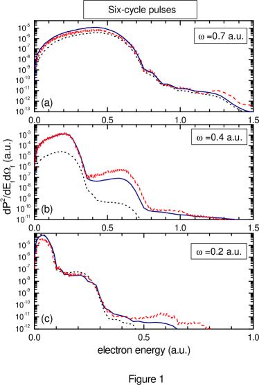
Figure 1: Differential electron emission probability, as a function of the electron energy, for the emission angle $\theta_{e}=$ $90^{\mathrm{\circ}}$. The parameters of the laser field are: $F_{0}=0.001$ $\mathrm{a.u.}$, (a) $\omega=0.7$ $\mathrm{a.u.}$, $\tau=54$ $\mathrm{a.u.,}$ (b) $\omega=0.4$ $\mathrm{a.u.,}$ $\tau=95$ $\mathrm{a.u.}$and (c) $\omega=0.2$ $\mathrm{a.u.,}$ $\tau=190$ $\mathrm{a.u.}$ Solid (blue) line, SJV results; dashed (red) line, TDSE values, and dotted line, results of the IJV model.

In Fig.1, six-cycle laser pulses with three different frequencies were considered: $\omega=0.7$, $0.4$ and $0.2$ $\mathrm{a.u..}$ In all the cases, to analyze the effect of the surface response on the electronic spectra SJV and TDSE values were compared to data derived within the previous IJV approach Fara07 , which neglects the contribution of $V_{ind}$. In Fig.1 (a) we show the emission probability corresponding to the frequency $\omega=0.7$ $\mathrm{a.u}$., which is higher than the surface plasmon frequency. For this frequency a good agreement between SJV and TDSE results is found. The SJV curve runs very close to TDSE values, showing only a small underestimation of TDSE results in high-velocity range. Note that both theories present a broad maximum, which can be associated with the above threshold ionization process. From the comparison to values obtained within the IJV approximation, we observe that for this high frequency the induced potential produces only a slight increment of the probability at low electron energies, having small influence on the overall electronic spectrum. However, when $\omega$ becomes resonant with the surface plasmon frequency, as in Fig.1 (b), the induced potential contributes greatly to increase the ionization probability in the whole energy range. Energy distributions obtained with SJV and TDSE methods are more than one order of magnitude higher than the one derived from the IJV approach. In this case SJV results follows quantitatively well the behavior of the TDSE curve, describing properly the positions of the multiphoton maxima but underestimating TDSE probabilities around the second peak. Note that in this case $V_{ind}$ does not represent a weak perturbation of the laser field, as shown in Fig.2(b) and it might be the origin of the observed discrepancy. In Fig.1 (c) we plot the emission probability for a laser field with a frequency $\omega=0.2$ $\mathrm{a.u.}$, lower than the plasmon one. Again, as in Fig.1 (a) SJV and TDSE results run very close to each other, displaying almost no differences with the IJV theory, which does not contain the induced potential. This indicates that the induced potential strongly affects emission spectra for frequencies resonant with the surface plasmon frequency, while for small deviations from this frequency it plays a minor role in the multiphoton ionization process.

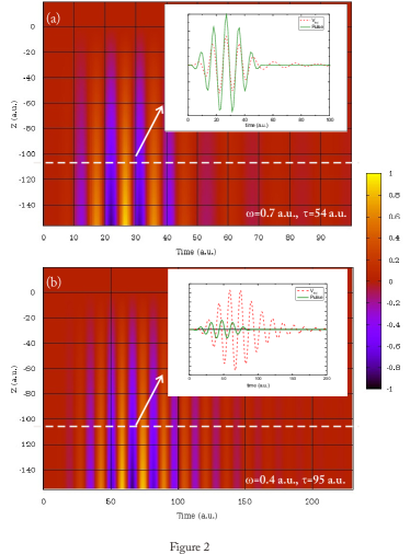
Figure 2: 2D-Representation of the induced potential, as a function of time and space. Laser pulse parameters are similar to Fig.1(a) and (b). Inset figures correspond to a given position inside the solid, with solid line, the laser pulse curve, and dashed line, the induced potential.

With the aim of examinating in detail the contribution of the induced potential, in Fig.2 we plot $V_{ind}$ as a function of time, for a given position inside the solid and for the frequencies of Fig.1(a) and (b). We observe that for $\omega=0.7$ a.u. the induced potential tends to follow the oscillations of the external field and its intensity steeply diminished when the pulse is turned off. Then, in this case the collective response of the medium produces only a weak effect on the electronic spectrum, as shown in Fig.1(a). Whereas for laser frequencies near to $\omega_{s}$ (Fig.2 (b)) the process is dominated by the induced potential, which produces an increment of the emission probability, as observed in Fig.1(b).

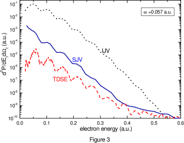
Figure 3: Similar to Fig.1. Laser field with $F_{0}=0.001$ $\mathrm{a.u.,}$ frequency $\omega=0.057$ $\mathrm{a.u.}$ and duration $\tau=660$ $\mathrm{a.u.}$

Finally, in Fig.3 we study a six-cycle laser pulse with the frequency corresponding to the experimental value for the Ti:sapphire laser system Miaja08 ( $\omega=0.057$ a.u.). For this low frequency, almost one order of magnitude lower than the plasmon one, the surface response approximates to the static limit and electronic fluctuations screen strongly the external field inside the solid. By comparing SJV and IJV results it is observed that in this case the induced potential contributes to reduce markedly the emission probability, up to two orders of magnitude at low electron energies. On the other hand, it should be noted that although the SJV theory describes properly the positions of multiphotonic maxima, it overestimates the emission probability given by the TDSE method. Such a discrepancy, which arises when $\omega$ is lower than the mean energy of initial bound electrons, was also observed for other Volkov-type methods applied to photoionization of atomic targets Macri03 .

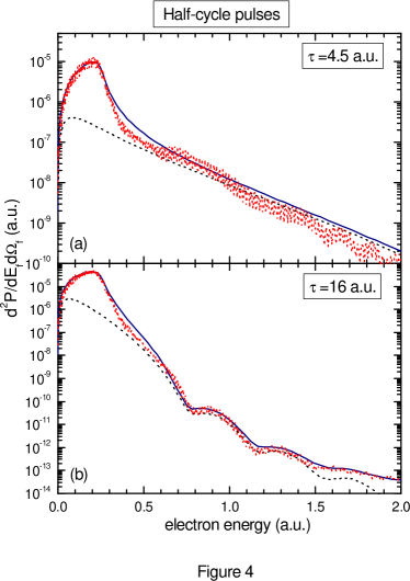
Figure 4: Similar to Fig.1. Half-cycle pulse with $F_{0}=0.001$ $\mathrm{a.u.,}$ (a) frequency $\omega=0.7$ $\mathrm{a.u.}$ and duration $\tau=4.5$ $\mathrm{a.u.,}$ (b) frequency $\omega=0.2$ $\mathrm{a.u.}$ and duration $\tau=16$ $\mathrm{a.u..}$

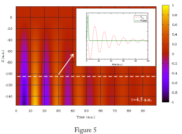
Figure 5: Similar to Fig.2. Laser field with $F_{0}=0.001$ $\mathrm{a.u.,}$ $\omega=0.7$ $\mathrm{a.u.}$ and $\tau=4.5$ $\mathrm{a.u..}$

To complete the previous analysis we reduce the duration of the pulse in order to investigate the contribution of the induced potential for photoelectron emission in the collisional regime Macri03 . In this regime, associated  with half-cycle pulses, the electromagnetic field does not oscillate, producing a perturbation similar to the one resulting of the interaction with a swift ion impinging grazingly on the surface (collision process).  Notice that for such ultrashort pulses the carrier frequency  $\omega$ loses its meaning and the pulse can be characterized by the sudden momentum transferred to the ejected electron, $\Delta p=-A^{-}(0)/c\simeq F_{0}\tau/2$ Arbo09 . In Fig.4 we plot electron distributions for half-cycle pulses with two different durations $\tau=4.5$   and $16\ \mathrm{a.u}$. In both cases we found a good agreement between SJV and TDSE methods in the whole electron velocity range. Both theories present a pronounced maximum at low electron velocities, which does not appear in the electron distribution derived from the IJV approach, being produced by the induced potential. To understand the origin of this increment of the probability at low electron energies, in Fig.5 we plot again the induced potential for a given position inside the solid, now for the case of Fig.4 (a).  We observe that for half-cycle pulses, without oscillations, after the pulse has finished the induced potential still affects solid electrons during at least a hundred atomic units more. This effect is the main source of electrons emission at low velocities.

III.1 Conclusions

In the present work we have introduced the SJV approximation, which allowed us to investigate the effects of the induced potential on the electron emission process. The proposed theory was compared to values derived from the numerical solution of the corresponding TDSE, displaying a good description of the main characteristics of photoemission spectra in the whole range of studied frequencies and durations of the laser pulse. From the comparison between SJV probabilities and those derived from the previous IJV approach, which does not include $V_{ind}$, we conclude that the induced potential can play an important role in laser-induced electron emission from metal surfaces, as expected. For laser pulses with several oscillations inside the envelope, we found that the induced potential produces a considerable increment of the probability when the laser frequency is resonant with the surface plasmon one, but as $\omega$ diminishes tending to the static case, the surface electronic density shields the laser field inside the solid,  leading to a markedly reduction of the photoemission process. In addition, for electromagnetic pulses in the collisional regime, the contribution of the surface induced potential after the pulse turns off gives rise to a maximum in the emission spectrum at low energies.

IV Acknowledgment

This work was done with the financial support of Grants UBACyT, ANPCyT and CONICET of Argentina. I. A, A. A. and V. M. S. gratefully acknowledge financial support by GU-UPV/EHU (grant no. IT-366-07) and MCI (grant no. FIS2007-66711-C02-02). The work of V.M.S is sponsored by the IKERBASQUE foundation.

References

- (1) A. L. Cavalieri, et al. Nature (London), 449, 1029 (2007).
- (2) E. Goulielmakis, V. S. Yakovlev, A. L. Cavalieri, M. Uiberacker, V. Pervak, A. Apolonski, R. Kienberger, U. Kleineberg, F. Krausz, Science 317, 769 (2007).
- (3) R. Kienberger et al. Nature (London), 427, 817 (2004).
- (4) C. A. Haworth, L. E. Chipperfield, J. S. Robinson, P. L. Knight, J. P. Marangos and J. W. G. Tisch, Nature Physics 3, 52 (2007).
- (5) A. Baltuska, et al. Nature (London) 421, 611 ( 2003).
- (6) E. Lorin, S. Chelkowski and A. D. Bandrauk, New Journal of Physics 10, 025033 (2008).
- (7) D. B. Milos̆ević, G. G. Paulus, D. Bauer and W. Becker, J. Phys. B 39, R203 (2006).
- (8) M. F. Kling, J.Rauschenberger, A. J. Verhoef, E. Hasovic, T. Uphues, D.B. Milosevic, H. G. Muller and M.J.J. Vrakking, New Journal of Physics 10, 025024 (2008).
- (9) L. Miaja-Avila et al. Phys. Rev. Lett. 101, 046101 (2008).
- (10) C. Lemell, B. Solleder, K. Tőkési, and J. Burgdörfer, Phys. Rev. A. 79, 062901 (2009).
- (11) D. M. Volkov, Z. Phys. 94, 250 (1935).
- (12) F..H. M. Faisal, J. Z. Kamiński and E. Saczuk, Phys. Rev. A. 72, 023412 (2005).
- (13) M. N. Faraggi, M. S. Gravielle and D. M. Mitnik, Phys. Rev. A 76, 012903 (2007).
- (14) J.C. Baggesen and L.B. Madsen, Phys. Rev. A 78, 032903 (2008).
- (15) C.-H. Zhang and U. Thumm, Phys. Rev. Lett. 102, 123601 (2009).
- (16) M.S. Gravielle and J.E. Miraglia, Phys. Rev. A 65, 022901 (2002).
- (17) P. Kurpick, U. Thumm and U. Wille, Phys. Rev. A 56, 543-554 (1997).
- (18) M. S. Gravielle, Phys. Rev. A 58, 4622 (1998).
- (19) M. Alducin, V. M. Silkin, J.I. Juaristi and E. V. Chulkov, Phys. Rev A 67, 032903 (2003).
- (20) P. Dombi, F. Krausz and G. Farkas, J. Mod. Optics 53,163 (2006).
- (21) D. P. Dewangan and J. Eichler, Phys. Rep. 247, 59-219 (1997).
- (22) W. H. Press, S. A. Teukolsky, W.T. Vetterling and B.P. Flannery, Numerical Recipes (Cambridge University Press, New York, 1992).
- (23) G. Saathoff, L. Miaja-Avila, M. Aeschlimann, M. M. Murnane, and H.C. Kapteyn, Phys. Rev. A 77, 022903 (2008).
- (24) L. Miaja-Avila, J. Yin, S. Backus, G. Saathoff, M. Aeschlimann, M. M. Murnane, and H.C. Kapteyn, Phys. Rev. A 79, 030901(R) (2009).
- (25) L.V. Keldysh, Sov. Phys. JETP 20, 1307 (1965).
- (26) P. Macri, J. E. Miraglia and M. S. Gravielle, J. Optical Society of America B 20, 1801 (2003).
- (27) D.G. Arbó, K. Tőkési and J.E. Miraglia, Nucl. Instr. and Meth. B 267, 382 (2009).