Production of two gluons in the Lipatov effective action formalism

Abstract

The one-loop diffractive amplitude for emission of two real gluons with widely different rapidities is studied in the Lipatov effective action formalism. It is shown that after integration over longitudinal momenta in the loop the resulting expression coincides with the one obtained by the Lipatov-Bartels formalism in transversal space provided the same prescription is used to exclude divergent contributions as previously proposed for emission of a single real gluon.

1 Introduction

In the framework of the perturbative QCD, in the Regge kinematics, particle interaction is described by the exchange of reggeized gluons which emit and absorb real gluons with certain production vertexes (”Lipatov vertexes’) [1]. Pomeron interaction leads to their splitting. Emission of real gluons from split reggeized gluons is described by vertexes introduced by J.Bartels (”Bartels vertexes’)  [2]. Originally both type of vertexes were calculated directly from the relevant simple Feynman diagrams in the Regge kinematics. Later a powerful effective action formalism was proposed by L.N.Lipatov  [3], which considers reggeized and normal gluons as independent entities from the start and thus allows to calculate all QCD diagrams in the Regge kinematics automatically and in a systematic and self-consistent way. However the resulting expressions are 4-dimensional and need reduction to the final 2-dimensional transverse form.

In the paper of two co-authors of the present paper (M.A.B. amd M.I.V.)  [4] it was demonstrated that the diffractive amplitude for the production of a real gluon calculated by means of the Lipatov effective action, after integration over the longitudinal variables, goes over into the expression obtained via the Lipatov and Bartels vertexes. However in the process of reduction to the transverse form a certain prescription had to be used to give sense to divergent integrals.

In this paper we generalize these results to a more complicated case of production of two real gluons with a large difference in rapidity. This case is of importance in view of the contradiction between the results obtained by Yu.Kovchegov and K.Tuchin  [5], on the one hand, and J.Bartels, M.Salvadore and G.P.Vacca  [6], on the other for the inclusive cross-section of gluon production in the Regge kinematics. Analysis of these results requires to compare expressions for the two-gluon production amplitude in the Lipatov-Bartels and dipole pictures. The study of this amplitude in the Lipatov effective action formalism is thus a valuable test of the presently used expressions.

Our results demonstrate that the Lipatov effective action leads to the standard expression for the two gluon production amplidude with the Lipatov and Bartels vertexes, provided the same prescription for the longitudinal integration is used as in  [4].

2 The set of diagrams

Our purpose is to study the amplitude for the production of two gluons in the diffractive collision on a colorless target. To simplify we shall restrict ourselves with a case when both colliding particle are quarks. This will introduce infrared divergence in the final intergrations over the transferred transverse momenta, absent with the realistic colorless participants. However our final goal is only to obtain the amplitudes with fixed transverse variables to be able to compare with the corresponding expression in the Lipatov-Bartels formalism. For this particular purpose using quarks as the projectile and target is sufficient. And it substancially reduces the number of diagrams to study.

Contributions to the process we study start at the perturbative order $g^{6}$, with which we limit ourselves here. All relevant diagrams then can be split into three groups shown in Figs. 1,2,3. Reggeized gluons are shown by wavy lines. The first group (1) consists of diagrams in which one gluon (the harder) is emitted before the reggeized gluon splits into two and the other at the splitting vertex. The second group (2) represents diagrams in which the harder gluon is emitted at the splitting vertex. Finally the third group (3) is represented by digrams in which the reggeized gluons do not split at all. Note that the contribution from the diagrams in which the harder gluon is emitted before splitting and the softer after splitting is equal to zero, since the splitting vertex without emission of a real gluon vanishes due to signature conservation.

We denote the momentum of the incident quark $k$ and that of the target quark $l$. Their final momenta are $k^{\prime}$ and $l^{\prime}$ respectively. We assume that $k_{-}=k_{\perp}=l_{+}=l_{\perp}=0$. The momenta of the emitted gluons are $p_{1}$ and $p_{2}$ with $p_{1+}>>p_{2+}$. For all longitudinal components we use the definition $a_{\pm}=a_{0}\pm a_{3}$, so that $ab=\frac{1}{2}a_{+}b_{-}+\frac{1}{2}a_{-}b_{+}+(ab)_{\perp}$.

In order to have the uniform notations for all diagrams we used the following definitions of various transferred momenta:

$$q=k-k^{\prime},\ \ q_{2}=q-p_{1}-q_{1},\ \ q_{3}=q-p_{1}-p_{2}-q_{1},\ \ q_{4}=q-p_{1},\ \ q_{5}=q-q_{1},\ \ q_{6}=q-q_{2}\,,$$ (1)

where $q_{1}$ is a loop momentum. In the Regge kinematics we have:

$$\sqrt{s}=k_{+}\approx k^{\prime}_{+}\gg p_{1+}\sim q_{+}\gg p_{2+}\sim q_{4+}\gg l^{\prime}_{+}$$

$$\sqrt{s}=l_{-}\approx l^{\prime}_{-}\gg p_{2-}\gg p_{1-}\sim-q_{4-}\gg k^{\prime}_{-}$$

$$q_{5+}\ll\sqrt{s},q_{6+}\ll\sqrt{s},q_{1-}\ll\sqrt{s},q_{2-}\ll\sqrt{s}\,.$$ (2)

We recall that in the Regge kinematics non-zero tranversal momentum components are assumed to be much smaller than longitudinal ones.

3 Diagram of Fig. 1

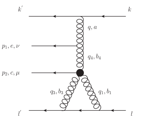
Figure 1: Diagram of the type 1

The only diagram of type 1 is shown in Fig. 1. We denote the wave functions of the projectile and target as $\bar{u}(k^{\prime})$, $u(k)$ and $\bar{w}(l^{\prime})$, $w(l)$ correspondingly. So the factors describing the projectile and target quarks are correspondingly

$$ig\bar{u}(k^{\prime})\frac{\gamma_{+}}{2}t^{a}u(k)$$ (3)

and

$$(ig)^{2}\bar{w}(l^{\prime})t^{b_{3}}\frac{\gamma_{-}}{2}\frac{i(\hat{l}+\hat{q_{1}})}{(l+q_{1})^{2}+i0}\frac{\gamma_{-}}{2}t^{b_{1}}w(l)\,.$$ (4)

We can use (2) to simplify

$$\gamma_{-}(\hat{l}+\hat{q_{1}})\gamma_{-}=\frac{1}{2}\gamma_{-}(l_{-}+q_{1-})\gamma_{+}\gamma_{-}=2\gamma_{-}(\sqrt{s}+q_{1-})\approx 2\sqrt{s}\gamma_{-}\,.$$ (5)

We shall be interested in the diffraction process when the target does not change its colour and so the $t$-channel coupled to the target is colourless. So we introduce a projector onto the colourless target state

$$P_{b_{1}b_{3}|b^{\prime}_{1}b^{\prime}_{3}}=\frac{\delta_{b_{1}b_{3}}\delta_{b^{\prime}_{1}b^{\prime}_{3}}}{N_{c}^{2}-1}\,.$$ (6)

Acting on the target quark colours it gives a factor

$$\frac{1}{N_{c}^{2}-1}\delta_{b^{\prime}_{1}b^{\prime}_{3}}t^{b^{\prime}_{3}}t^{b^{\prime}_{1}}=\frac{1}{2N_{c}}\,.$$ (7)

The diagram of Fig. 1 is formed by the vertexes already studied previously. The lower vertex is the Reggeon $\to$ 2 Reggeons + Particle (”effective”) vertex obtained in  [4]:

$$\begin{split}\frac{ig^{2}f^{b_{3}cd}f^{b_{4}b_{1}d}}{(q_{4}-q_{1})^{2}}\left[q_{4+}(q_{4}\varepsilon^{*}_{2})_{\bot}+\frac{q_{4}^{2}}{q_{1-}}\left(-((q_{4}-q_{1})\varepsilon^{*}_{2})_{\bot}+\frac{(q_{4}-q_{1})^{2}}{p_{2\bot}^{2}}(p_{2}\varepsilon^{*}_{2})_{\bot}\right)\right]\\ +\frac{ig^{2}f^{b_{1}cd}f^{b_{4}b_{3}d}}{(q_{4}-q_{3})^{2}}\left[q_{4+}(q_{4}\varepsilon^{*}_{2})_{\bot}+\frac{q_{4}^{2}}{q_{3-}}\left(-((q_{4}-q_{3})\varepsilon^{*}_{2})_{\bot}+\frac{(q_{4}-q_{3})^{2}}{p_{2\bot}^{2}}(p_{2}\varepsilon^{*}_{2})_{\bot}\right)\right]\,.\end{split}$$ (8)

The third term in each square brackets is the contribution of the so-called ”induced” vertex which is given by expansion of the $P$-exponential in the effective action [3].

The upper vertex is the well-known Reggeon $\to$ Reggeon $+$ particle (”Lipatov”) vertex, which we write as:

$$igf^{ab_{4}e}q_{\bot}^{2}\Big{(}L_{\perp}(q,p_{1})\varepsilon^{*}_{1}\Big{)}\,,$$ (9)

where we define the transverse vector

$$L_{\nu}(q,p)=\frac{q_{\bot\nu}}{q^{2}_{\bot}}-\frac{p_{\bot\nu}}{p^{2}_{\bot}}\,.$$ (10)

The effective vertex consists of two parts proportional to $f^{b_{3}cd}f^{b_{4}b_{1}d}$ and and $f^{b_{1}cd}f^{b_{4}b_{3}d}$, each containing three terms. In both cases the convolution of the vertex colour factors with the target colour factor (7) gives the final overall colour factor

$$\frac{1}{2N_{c}}f^{ab_{4}e}f^{b_{1}cd}f^{b_{4}b_{1}d}t^{a}=\frac{1}{2}f^{aec}t^{a}\,.$$ (11)

To reduce the contribution of the diagram to the 2-dimensional form we have to integrate over the longitudinal variables in the loop. This integration does not involve the four reggeon propagators as they are purely transversal

$$D^{ab}(q)=-i\frac{2\delta_{ab}}{q^{2}_{\bot}}$$ (12)

and thus contribute a totally transverse factor

$$\frac{16}{q^{2}_{\bot}q^{2}_{4\bot}q^{2}_{1\bot}q^{2}_{3\bot}}\,.$$ (13)

The effective vertex generates three kinds of terms including longitudinal components proportional to

$$q_{4+}(q_{4}\varepsilon^{*}_{2})_{\bot}\,,$$ (14)

$$\frac{q_{4}^{2}}{q_{i-}}(-((q_{4}-q_{i})\varepsilon^{*}_{2})_{\bot}),\ \ i=1,3$$ (15)

and

$$\frac{q_{4}^{2}}{q_{i-}}\frac{(q_{4}-q_{i})^{2}}{p_{2\bot}^{2}}(p_{2}\varepsilon^{*}_{2})_{\bot},\ \ i=1,3\,.$$ (16)

Combined with the denominator from the quark propagator the first two terms lead to the longitudinal integrals of two forms

$$J_{1}(k_{1},k_{2})=\frac{1}{2i}\int\frac{dq_{1-}}{2\pi}\int\frac{dq_{1+}}{2\pi}\frac{1}{(k_{1}^{2}+i0)(k_{2}^{2}+i0)}$$ (17)

and

$$J_{2}(k,k_{1},k_{2})=\frac{1}{2i}\int\frac{dq_{1-}}{2\pi}\int\frac{dq_{1+}}{2\pi}\frac{1}{k_{-}}\frac{1}{(k_{1}^{2}+i0)(k_{2}^{2}+i0)}\ .$$ (18)

where $k$, $k_{1}$ and $k_{2}$ are some linear functions of the integration momentum $q_{1}$.

The first terms, proportional to (14), lead to the integrals

$$I_{1}=J_{1}(q_{4}-q_{1},l+q_{1})$$ (19)

and

$$I_{2}=J_{1}(q_{4}-q_{3},l+q_{1})\,.$$ (20)

The second terms (15) combined with the target quark denominator lead to the integrals

$$I_{3}=J_{2}(q_{1},q_{4}-q_{1},l+q_{1})$$ (21)

and

$$I_{4}=J_{2}(q_{3},q_{4}-q_{3},l+q_{1})\,.$$ (22)

The third terms (16) combined with the target quark propagator give the integrals

$$\frac{1}{2i}\int\frac{dq_{1-}}{2\pi}\int\frac{dq_{1+}}{2\pi}\frac{1}{q_{1-}}\frac{1}{(l+q_{1})^{2}+i0}$$ (23)

and

$$\frac{1}{2i}\int\frac{dq_{1-}}{2\pi}\int\frac{dq_{1+}}{2\pi}\frac{1}{q_{3-}}\frac{1}{(l+q_{1})^{2}+i0}\ .$$ (24)

In these formulas $q_{3}=q-p_{1}-p_{2}-q_{1}$.

The first four integrals (19-22) are calculated in the Appendix. The last integrals (23), (24) are formally divergent. The same integrals were also found in the simpler case of the single gluon production in  [4]. There it was noted that if a prescription is imposed to calculate the integral in the principal value sense then the integral vanishes and the result turns out to be in agreement with the standard Lipatov-Bartels approach in terms of ordinary Feynman diagrams. Relying on this conclusion we also in this study impose the same rule of calculation and consequently neglect these integral altogether.

The results found in the Appendix for the sum of the first two integrals is

$$I_{1}+I_{2}=\frac{i}{4q_{4+}\sqrt{s}}\,,$$ (25)

attaching the rest factor from the effective vertex we find the total contribution to the diagram from the terms (14) as

$$\frac{i(q_{4}\varepsilon^{*}_{2})_{\bot}}{4\sqrt{s}}\ .$$ (26)

For the second terms, the factors (15) are different for the two parts of the effective vertex. If we change the variable of the loop integration $q_{1}\to q_{3}=q-p_{1}-p_{2}-q_{1}$ only in the contribution of the second part, then the factors (15) become equal and we need to calculate the sum of integrals $I_{3}$ and $I_{4}=J_{2}(q_{1},q_{4}-q_{1},l^{\prime}-q_{1})$. The sum of integrals is found to be

$$I_{3}+I_{4}=\frac{i}{4\sqrt{s}(q_{4}-q_{1})^{2}_{\bot}}\ .$$ (27)

Combined with the rest factor from the effective vertex they give the contribution from the terms (15) as

$$-\frac{iq_{4\bot}^{2}}{4\sqrt{s}(q_{4}-q_{1})^{2}_{\bot}}((q_{4}-q_{1})\varepsilon^{*}_{2})_{\bot}\ .$$ (28)

Summing (26) and (28) we find the final result for the diagram of type 1 in the form

$$g^{6}\cdot\bar{u}(k^{\prime})\gamma_{+}\Delta_{1}u(k)\cdot\bar{w}(l^{\prime})\gamma_{-}w(l)\,,$$ (29)

where

$$\Delta_{1}=\frac{i}{2}f^{aec}t^{a}\cdot\int\frac{d^{2}q_{1\bot}}{(2\pi)^{2}}\frac{1}{q^{2}_{1\bot}}\frac{1}{q^{2}_{3\bot}}\left(L_{\bot}(q,p_{1})\varepsilon^{*}_{1}\right)\left(B_{\bot}(q_{4},q_{2})\varepsilon^{*}_{2}\right)\,.$$ (30)

Here we denoted

$$B_{\nu}(q,p)=\frac{q_{\bot\nu}}{q^{2}_{\bot}}-\frac{p_{\bot\nu}}{p^{2}_{\bot}}$$ (31)

with

$$q_{2}=q_{4}-q_{1}=q-p_{1}-q_{1},\ \ q_{3}=q-p_{1}-p_{2}-q_{1}\,.$$ (32)

This is the momentum part of the well-known Bartels vertex [2] expressed in terms of this part for the Lipatov vertex. Expression (30) is exactly the one which is found for the configuration of the diagram in Fig. 1 in the Lipatov-Bartels formalism using the transverse space approach from the start.

4 Diagrams of Fig. 2

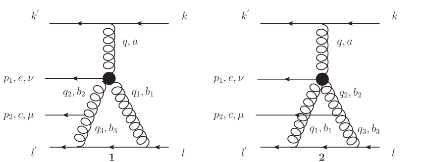
Figure 2: Diagrams of the type 2

The two diagrams of type 2 are shown in Fig. 2. The softer gluon is now emitted from inside the loop. The structure of the diagrams is similar to the previous case except that the effective vertex has the larger rapidity than the Lipatov vertex.

The target factor for the diagram Fig. 2.1 is

$$\bar{w}(l^{\prime})t^{b_{3}}\frac{ig\gamma_{-}}{2}\frac{i(\hat{l}+\hat{q_{1}})}{(l+q_{1})^{2}+i0}\frac{ig\gamma_{-}}{2}t^{b_{1}}w(l)$$ (33)

and for the diagram Fig. 2.2 is

$$\bar{w}(l^{\prime})t^{b_{1}}\frac{ig\gamma_{-}}{2}\frac{i(\hat{l^{\prime}}-\hat{q_{1}})}{(l^{\prime}-q_{1})^{2}+i0}\frac{ig\gamma_{-}}{2}t^{b_{3}}w(l)\,.$$ (34)

Similar to (5):

$$\gamma_{-}(\hat{l^{\prime}}-\hat{q_{1}})\gamma_{-}\approx 2\sqrt{s}\gamma_{-}\ .$$ (35)

Reggeon propagators give a factor

$$\frac{16}{q^{2}_{\bot}q^{2}_{1\bot}q^{2}_{2\bot}q^{2}_{3\bot}}\ .$$ (36)

For the first diagram Fig. 2.1 the effective vertex is

$$\frac{ig^{2}f^{b_{1}ed}f^{ab_{2}d}}{(q-q_{2})^{2}}\left[q_{+}(q\varepsilon^{*}_{1})_{\bot}+\frac{q^{2}}{q_{2-}}\left(-((q-q_{2})\varepsilon^{*}_{1})_{\bot}+\frac{(q-q_{2})^{2}}{p_{1\bot}^{2}}(p_{1}\varepsilon^{*}_{1})_{\bot}\right)\right]$$

$$+\frac{ig^{2}f^{b_{2}ed}f^{ab_{1}d}}{(q-q_{1})^{2}}\left[q_{+}(q\varepsilon^{*}_{1})_{\bot}+\frac{q^{2}}{q_{1-}}\left(-((q-q_{1})\varepsilon^{*}_{1})_{\bot}+\frac{(q-q_{1})^{2}}{p_{1\bot}^{2}}(p_{1}\varepsilon^{*}_{1})_{\bot}\right)\right]\ .$$ (37)

and the Lipatov vertex is

$$igf^{b_{2}b_{3}c}q_{2\bot}^{2}\left(L_{\bot}(q_{2},p_{2})\varepsilon^{*}_{2}\right)=igf^{b_{2}b_{3}c}q_{2\bot}^{2}\left(\frac{(q_{2}\varepsilon^{*}_{2})_{\bot}}{q^{2}_{2\bot}}-\frac{(p_{2}\varepsilon^{*}_{2})_{\bot}}{p^{2}_{2\bot}}\right)\ .$$ (38)

For the second diagram Fig. 2.2 the effective vertex is the same (37), since it is invariant under interchange of the two lower reggeons, and the Lipatov’s vertex is also (38).

The projection of the reggeons coupled to the target onto the colorless state supplies the same factor as for the diagram of Fig. 1 (6). Its convolution with other color factors for both digarams of Fig. 2 however gives different results for the two parts of the effective vertex. For the first part we get

$$\frac{1}{2N_{c}}f^{b_{1}ed}f^{ab_{2}d}f^{b_{2}b_{1}c}t^{a}=-\frac{1}{4}f^{aec}t^{a}$$ (39)

and for the second part we get the opposite sign

$$\frac{1}{2N_{c}}f^{b_{2}ed}f^{ab_{1}d}f^{b_{2}b_{1}c}t^{a}=\frac{1}{4}f^{aec}t^{a}\,.$$ (40)

Further calculations are quite similar to those for the diagram on Fig. 1, except that now we have to consider the two parts of the effective vertex separately. In the following we choose the integration variable to be $q_{1}$.

Consider the diagram Fig. 2.1. The first terms in the two parts of the effective vertex lead to the integrals respectively

$$I_{5}=J_{1}(q-q_{2},l+q_{1})=0$$ (41)

and

$$I_{6}=J_{1}(q-q_{1},l+q_{1})=\frac{i}{4q_{+}\sqrt{s}}\,.$$ (42)

Notice that $I_{5}$ enters with the color factor (39) and $I_{6}$ does with the color factor (40). For the second diagram Fig. 2.2 the integrals for the first terms of the effective vertex are

$$I_{7}=J_{1}(q-q_{2},l^{\prime}-q_{1})=\frac{i}{4q_{+}\sqrt{s}}$$ (43)

and

$$I_{8}=J_{1}(q-q_{1},l^{\prime}-q_{1})=0$$ (44)

and the color factors are (39) and (40) respectively. Since the contributions of the two non-zero integrals enter with the opposite sign, in the sum of the two diagrams in Fig. 2 we get zero.

The last terms in the effective vertex again formally diverge. Using our prescription of the principal value integration we put them to zero. So in the end only the second terms in the effective vertex give non-zero contribution.

For the first diagram in Fig. 2 they lead to the longitudinal integrals $I_{9}=J_{2}(q_{2},q-q_{2},l+q_{1})$ and $I_{10}=J_{2}(q_{1},q-q_{1},l+q_{1}).$ For the second diagram in Fig. 2 one has to change $l+q_{1}\to l^{\prime}-q_{1}$: $I_{11}=J_{2}(q_{2},q-q_{2},l^{\prime}-q_{1})$ and $I_{12}=J_{2}(q_{1},q-q_{1},l^{\prime}-q_{1}).$

The integrals are similar to that we have calculated for diagram in Fig. 1. Color factor (39) corresponds to $I_{9}$ and $I_{11}$. Summing them we obtain

$$-\frac{1}{4}f^{aec}t^{a}(I_{9}+I_{11})=-\frac{1}{4}f^{aec}t^{a}\frac{i}{4(q-q_{2})^{2}_{\bot}}\,.$$ (45)

Similarly, the second part gives

$$\frac{1}{4}f^{aec}t^{a}(I_{10}+I_{12})=\frac{1}{4}f^{aec}t^{a}\frac{i}{4(q-q_{1})^{2}_{\bot}}\,.$$ (46)

Taking in account that vertex (38) is the same for both diagrams we obtain for the sum of diagrams Fig. 2:

$$g^{6}\cdot\bar{u}(k^{\prime})\gamma_{+}\Delta_{2}u(k)\cdot\bar{w}(l^{\prime})\gamma_{-}w(l)\,,$$ (47)

where

$$\Delta_{2}=\frac{i}{4}f^{aec}t^{a}\cdot\int\frac{d^{2}q_{1\bot}}{(2\pi)^{2}}\frac{1}{q^{2}_{1\bot}}\frac{1}{q^{2}_{3\bot}}\left[(B_{\bot}(q,q_{5})\varepsilon^{*}_{1})-(B_{\bot}(q,q_{6})\varepsilon^{*}_{1})\right]\left(L_{\bot}(q_{2},p_{2})\varepsilon^{*}_{2}\right)\,.$$ (48)

The definition of $B_{\nu}$ was made in (31). This result is also corresponding to the Lipatov-Bartels formalism.

5 Diagrams of Fig. 3

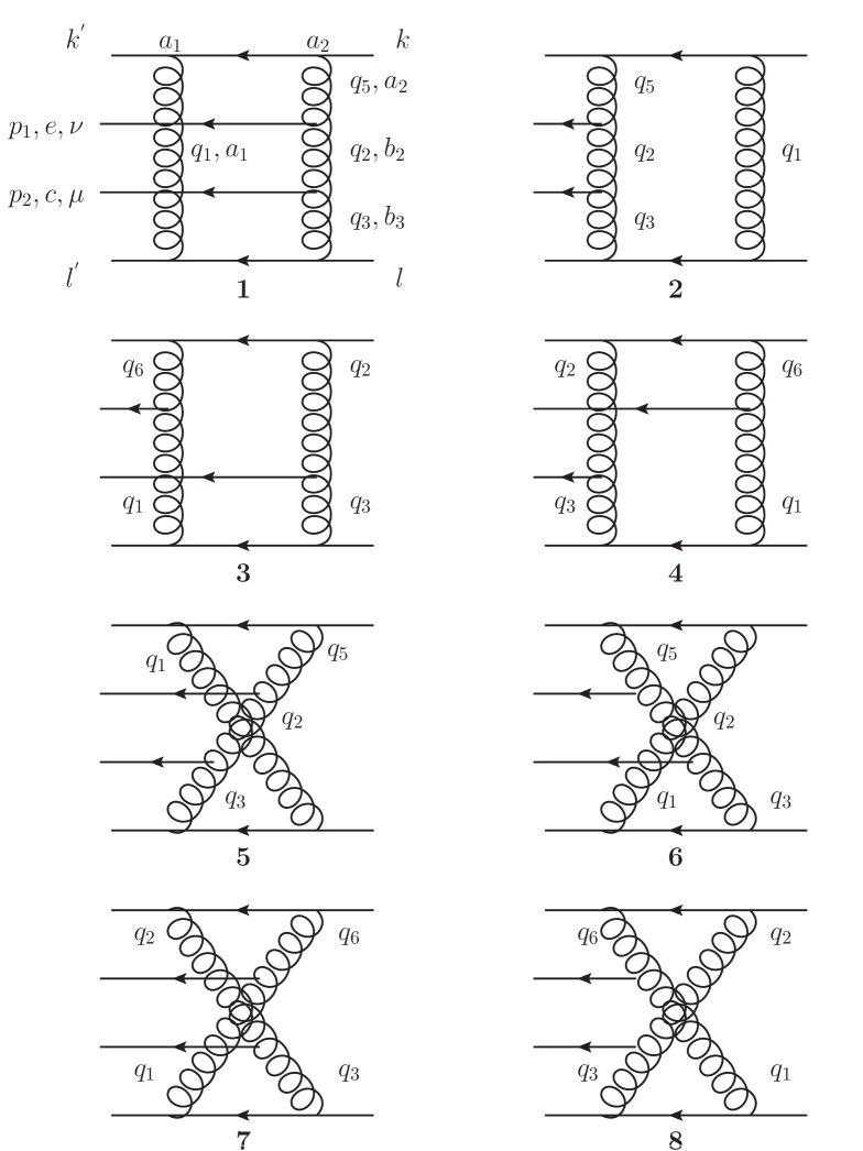
Figure 3: Diagrams of the type 3

The diagrams on Fig (3) divide into two parts: with emission of the two gluons from the same reggeon (diagrams 1,2,5 and 6) and from different reggeons (diagrams 3,4,7 and 8). These two parts have different structures of the Lipatov vertices. Consider diagram 1. Factors coupled with the target and projectile quarks are:

$$\bar{w}(l^{\prime})t^{a_{1}}\frac{ig\gamma_{-}}{2}\frac{i(\hat{l^{\prime}}-\hat{q_{1}})}{(l^{\prime}-q_{1})^{2}+i0}\frac{ig\gamma_{-}}{2}t^{b_{3}}w(l)$$ (49)

and

$$\bar{u}(k^{\prime})t^{a_{1}}\frac{ig\gamma_{+}}{2}\frac{i(\hat{k^{\prime}}+\hat{q_{1}})}{(k^{\prime}+q_{1})^{2}+i0}\frac{ig\gamma_{+}}{2}t^{a_{2}}u(k)\,.$$ (50)

As before we simplify

$$\gamma_{-}(\hat{l^{\prime}}-\hat{q_{1}})\gamma_{-}\approx 2\sqrt{s}\gamma_{-}\ ,$$ (51)

$$\gamma_{+}(\hat{k^{\prime}}+\hat{q_{1}})\gamma_{+}\approx 2\sqrt{s}\gamma_{+}\ .$$ (52)

The reggeon propagators are:

$$\frac{16}{q^{2}_{1\bot}q^{2}_{2\bot}q^{2}_{3\bot}q^{2}_{5\bot}}\,.$$ (53)

The two Lipatov vertices are:

$$igf^{a_{2}b_{2}e}q_{5\bot}^{2}\left(\frac{(q_{5}\varepsilon^{*}_{1})_{\bot}}{q^{2}_{5\bot}}-\frac{(p_{1}\varepsilon^{*}_{1})_{\bot}}{p^{2}_{1\bot}}\right)\,,$$ (54)

$$igf^{b_{2}b_{3}c}q_{2\bot}^{2}\left(\frac{(q_{2}\varepsilon^{*}_{2})_{\bot}}{q^{2}_{2\bot}}-\frac{(p_{2}\varepsilon^{*}_{2})_{\bot}}{p^{2}_{2\bot}}\right)\,.$$ (55)

After the projection of the reggeons coupled to the target onto the colorless state we obtain the following color structure:

$$\frac{1}{2N_{c}}f^{a_{2}b_{2}e}f^{b_{2}a_{1}c}t^{a_{1}}t^{a_{2}}\ .$$ (56)

The diagram 5 differs from this one only in the target quark propagator in which $l^{\prime}-q_{1}\to l+q_{1}$. The diagrams 2 and 6 have a different color structure

$$\frac{1}{2N_{c}}f^{a_{2}b_{2}e}f^{b_{2}a_{1}c}t^{a_{2}}t^{a_{1}}\ .$$ (57)

It is convenient to combine momentum parts of these four diagrams. In order to do it we split $t^{a_{1}}t^{a_{2}}$ into symmetric and antisymmetric parts:

$$t^{a_{1}}t^{a_{2}}=\frac{1}{2}\{t^{a_{1}},t^{a_{2}}\}+\frac{1}{2}[t^{a_{1}},t^{a_{2}}]$$ (58)

to obtain colour factors

$$\frac{1}{4N_{c}}f^{a_{2}b_{2}e}f^{b_{2}a_{1}c}[t^{a_{1}},t^{a_{2}}]=\frac{i}{8}f^{aec}t^{a}$$ (59)

$$\frac{1}{4N_{c}}f^{a_{2}b_{2}e}f^{b_{2}a_{1}c}\{t^{a_{1}},t^{a_{2}}\}=-\frac{1}{4N_{c}}\delta^{ce}-\frac{1}{8}d^{aec}t^{a}\ .$$ (60)

Thus for the antisymmetric part we use (59) with an extra minus sign for diagrams 2 and 6. For the total symmetric part we use (60) for all four diagrams.

The longitudinal integrals for diagrams 1, 2, 5 and 6 are correspondingly

$$I_{13}=J_{1}(k^{\prime}+q_{1},l^{\prime}-q_{1})=\frac{i}{4s}\,,$$ (61)

$$I_{14}=J_{1}(k-q_{1},l+q_{1})=\frac{i}{4s}\,,$$ (62)

$$I_{15}=J_{1}(k^{\prime}+q_{1},l+q_{1})=0\,,$$ (63)

$$I_{16}=J_{1}(k-q_{1},l^{\prime}-q_{1})=0\,.$$ (64)

As we observe, the antisymmetric part completely vanishes. In the symmetric part for the sum of diagrams 1, 2, 5 and 6 we obtain

$$2i\left(-\frac{\delta^{ce}}{4N_{c}}-\frac{d^{aec}}{8}t^{a}\right)\cdot\int\frac{d^{2}q_{1\bot}}{(2\pi)^{2}}\frac{1}{q^{2}_{1\bot}}\frac{1}{q^{2}_{3\bot}}\left(L_{\bot}(q_{5},p_{1})\varepsilon^{*}_{1}\right)\left(L_{\bot}(q_{2},p_{2})\varepsilon^{*}_{2}\right)\,.$$ (65)

Calculation of diagrams 3, 4, 7 and 8 is completely similar. The total result for all diagrams in Fig. 3 is

$$g^{6}\cdot\bar{u}(k^{\prime})\gamma_{+}\Delta_{3}u(k)\cdot\bar{w}(l^{\prime})\gamma_{-}w(l)\,,$$ (66)

where

$$\Delta_{3}=2i\left(-\frac{1}{4N_{c}}\delta^{ce}-\frac{1}{8}d^{aec}t^{a}\right)\cdot\int\frac{d^{2}q_{1\bot}}{(2\pi)^{2}}\frac{1}{q^{2}_{1\bot}}\frac{1}{q^{2}_{3\bot}}\left(L_{\bot}(q_{2},p_{2})\varepsilon^{*}_{2}\right)$$

$$\left[(L_{\bot}(q_{5},p_{1})\varepsilon^{*}_{1})-(L_{\bot}(q_{6},p_{1})\varepsilon^{*}_{1})\right]\,.$$ (67)

This expression is exactly the one obtained in the standard Lipatov-Bartels transverse space approach .

6 Conclusions

Using the Lipatov effective field theory we have generalized the results of  [4] to the case when in the diffractive process two real soft gluons are emiited with large distance between their rapidities The Reggeon $\to$ 2 Reggeons+Particle vertex involved in the process was taken from  [4]. The found general structure of the amplitude corresponds to what has been known from the direct calculation of standard Feynman diagrams. To check the full correspondence we performed longitudinal integrations. The encountered difficulties are the same as with the single gluon emission. They require imposition of a certain rule, which reduces to taking certain integrals in the prinicpal value recipe. With this rule obeyed, the found expression for the production amplitude completely coincides with the one obtained by using Lipatov and Bartels vertexes in the transversal space from the start.

It however remains to be seen if this result is true when the target changes its colour. Such a process is an important part of the inclusive soft gluon production, which is now under careful study in view of the contradiction betwen the results found in the Lipatov-Bartels and dipole pictures, mentioned in the introduction. We leave this problem for future studies.

7 Acknowledgements

This work has been partially supported by grants RNP 2.1.1/1575 of Education and Science Ministry of Russia and RFFI 09-02-01327a.

8 Appendix. Calculation of longitudinal integrals

The typical longitudinal integral of the form (17) is

$$I_{1}=J_{1}(q_{4}-q_{1},l+q_{1})=\frac{1}{2i}\int\frac{dq_{1-}}{2\pi}\int\frac{dq_{1+}}{2\pi}\frac{1}{[(q_{4}-q_{1})^{2}+i0]}\frac{1}{[(l+q_{1})^{2}+i0]}\ .$$ (68)

The standard procedure to calculate similar integrals is to use that the longitudinal components of the reggeon momentum $q_{1\pm}$ can be neglected as compared to large longitudinal components of the particles to which the reggeon is coupled, that is $q_{1+}$ is to be neglected as compared to $q_{4+}$ and $q_{1-}$ is to be neglected as compared to $l_{-}$. Should we follow this procedure, integral $I_{1}$ will factorize into two independent integrals over $q_{1+}$ and $q_{1-}$, but both of them will be divergent at large $q_{1\pm}$. Below we shall demonstrate that this procedure still can be applied not to separate integrals like (68) but to the sum of integrals coming from the direct and crossed terms in our expression and also somewhat transformed to achieve convergence. To be able to calculate separate integrals of our type we recur to a slightly different procedure, in which the condition that $q_{1\pm}$ are small is imposed not from the start but after integration in one of the longitudinal momenta. Of course our procedure is fully equivalent to the standard one applied to convergent integrals and gives identical results.

As a function of $q_{1+}$ the integrand has two poles

$$q_{1+}=q_{4+}-\frac{(q_{4}-q_{1})^{2}_{\bot}+i0}{q_{1-}}$$ (69)

and

$$q_{1+}=-\frac{(q_{1}+l)^{2}_{\bot}+i0}{q_{1-}+l_{-}}\ .$$ (70)

A non-zero result is obtained only if the two poles in $q_{1+}$ are on the opposite sides from the real axis. It determines the limits of the integration over $q_{1-}$. In the Regge kinematics in any case $q_{1-}<<l_{-}$ so that the limits are

$$-l_{-}<q_{1-}<0\,.$$ (71)

Thus taking the residue at (69) we get an integral over $q_{1-}$

$$\frac{1}{4\pi}\int_{-l_{-}}^{0}dq_{1-}\frac{1}{D_{1}}\ ,$$ (72)

where

$$D_{1}=q_{1-}^{2}q_{4+}+q_{1-}(l_{-}q_{4+}-(q_{4}-q_{1})^{2}_{\bot}+q_{1\perp}^{2})-l_{-}(q_{4}-q_{1})^{2}_{\perp}-i0\,.$$ (73)

The integral over $q_{1-}$ can be directly calculated as it stands. However such calculation is incorrect, since it does not take into account the kinematical conditions which are to be fulfilled for the propagating reggeons. In fact we have to require that both longitudinal components of the reggeon momenta are small as compared with the transversal components. Otherwise the longitudinal momenta have to be kept in the reggeon propagator and, if large, will correspond to the kinematics quite different to the Regge one. So we have to restrict integration in (68) to the region

$$|q_{1+}q_{1-}|<<|q_{1\perp}^{2}|\,.$$ (74)

In our case from (69) we have

$$q_{1+}q_{1-}=q_{4+}q_{1-}-(q_{4}-q_{1})_{\perp}^{2}\,,$$ (75)

so that condition (74) transforms into

$$|q_{4+}q_{1-}-(q_{4}-q_{1})_{\perp}^{2}|<<|q_{1\perp}^{2}|\ .$$ (76)

This implies that the integration in $q_{1-}$ is to be restricted to a narrow interval around the point where the left-hand side of (76) vanishes.

With small values of $q_{1-}$ of this order, we have to drop here all terms except by those which contain a large factor $l_{-}$, so that we get

$$D_{1}(q_{1-})=l_{-}\Big{(}q_{4+}q_{1-}-(q_{4}-q_{1})_{\perp}^{2}-i0\Big{)}\ ,$$ (77)

and according to (76) the integration should go in a small interval around the point where $D_{1}(q_{1-})=0$. This means that in fact

$$\frac{1}{D_{1}(q_{1-})}=\frac{i\pi}{l_{-}}\delta\Big{(}q_{4+}q_{1-}-(q_{4}-q_{1})_{\perp}^{2}\Big{)}\ .$$ (78)

Notice that $q_{4+}\approx p_{2+}>0$. Since $(q_{4}-q_{1})_{\perp}^{2}<0$ and in the integration region also $q_{4+}q_{1-}<0$ the $\delta$-function gives a nonzero contribution and we obtain

$$I_{1}=\frac{i}{4l_{-}q_{4_{+}}}\ .$$ (79)

Now take integral (20). First changing the integration variable to $q_{3}$ and then redenoting it as $q_{1}$ we find

$$I_{2}=J_{1}(q_{4}-q_{1},l^{\prime}-q_{1})=\frac{1}{2i}\int\frac{dq_{1-}}{2\pi}\int\frac{dq_{1+}}{2\pi}\frac{1}{[(q_{4}-q_{1})^{2}+i0]}\frac{1}{[(l^{\prime}-q_{1})^{2}+i0]}\ .$$ (80)

The two poles in $q_{1+}$ are now the old one (69) and

$$q_{1+}=l^{\prime}_{+}+\frac{(l^{\prime}-q_{1})_{\perp}^{2}+i0}{l^{\prime}_{-}-q_{1-}}\ .$$ (81)

Now the integration region in $q_{1-}$ is

$$0<q_{1-}<l^{\prime}_{-}\ .$$ (82)

We get an integral

$$I_{2}=-\frac{1}{4\pi}\int_{0}^{l^{\prime}_{-}}dq_{1-}\frac{1}{D_{2}}\,,$$ (83)

where

$$D_{2}(q_{1-})=q_{1-}^{2}(q_{4+}-l^{\prime}_{+})-q_{1-}(l^{\prime}_{-}q_{4+}+(q_{4}-q_{1})^{2}_{\bot}-(l^{\prime}-q_{1})^{2}_{\bot}+{l^{\prime}}_{\perp}^{2})+l^{\prime}_{-}(q_{4}-q_{1})^{2}_{\bot}+i0$$ (84)

and the minus sign is due to the fact that the pole (69) now lies in the upper half plane. According to our estimates, in the assumed kinematical conditions only the term in $D_{2}$ which contains $q_{1-}$ multiplied by $l^{\prime}_{-}q_{4+}$ is to be kept, so that

$$D_{2}(q_{1-})=l^{\prime}_{-}\Big{(}(q_{4}-q_{1})^{2}-q_{1-}q_{4_{+}}+i0\Big{)}$$ (85)

and according to (76) we have to integrate over $q_{1-}$ in the small interval around the point where $D_{2}(q_{1-})=0$. But now in (85) the right-hand side never vanishes, since in the brackets both terms are negative in the integration region. So we find

$$I_{2}=0$$ (86)

and the result (25) follows.

The integrals of the second form (18) $I_{3}$ and $I_{4}$ contain an extra factor $q_{1-}$ in the denominator as compared to $I_{1}$ and $I_{2}$. On the formal level this leads to a divergency of these two integrals at the point $q_{1-}=0$. However in the sum $I_{3}+I_{4}$ this divergence cancels. Indeed using our approximate expressions for $D_{1}$ and $D_{2}$ valid in the region (76) we find

$$I_{3}+I_{4}=\frac{1}{4\pi}\int_{0}^{l_{-}}\frac{dq_{1-}}{q_{1-}}\Big{(}-\frac{1}{D_{1}(-q_{1-})}-\frac{1}{D_{2}(q_{1-})}\Big{)}$$

$$=\frac{1}{4\pi l_{-}}\int_{0}^{l_{-}}\frac{dq_{1-}}{q_{1-}}\Big{(}\frac{1}{q_{4+}q_{1-}+(q_{4}-q_{1})_{\perp}^{2}+i0}-\frac{1}{(q_{4}-q_{1})_{\perp}^{2}-q_{1-}q_{4_{+}}+i0}\Big{)}\ .$$ (87)

Obviously the integrand is not singular at $q_{1-}=0$.

We have to integrate this expression in in the small interval around the points where $D_{1}=0$ or $D_{2}=0$. However, as we have seen, the denominator $D_{2}$ never vanishes. So in (87) we can drop the second term and in the first term change

$$\frac{1}{q_{4+}q_{1-}+(q_{4}-q_{1})_{\perp}^{2}+i0}\to-i\pi\delta\Big{(}q_{4+}q_{1-}+(q_{4}-q_{1})_{\perp}^{2})\Big{)}\ ,$$

which gives

$$I_{3}+I_{4}=\frac{i}{4l_{-}(q_{4}-q_{1})_{\perp}^{2}}$$ (88)

that is Eq. (27).

The rest of longitudinal integrals can be calculated in a similar manner.

Now we are going to demonstrate that one can also calculate our integrals in the standard manner, factorizing them into two independent ones over $q_{1\pm}$. Take integral $I_{1}$. As mentioned one cannot neglect $q_{1+}$ in the first denominator and $q_{1-}$ in the second without losing convergence. To preserve it we consider the sum of integrals (19) and (20)

$$I_{1}+I_{2}=\frac{1}{2i}\int\frac{dq_{1-}}{2\pi}\int\frac{dq_{1+}}{2\pi}\Big{\{}\frac{1}{(q_{4}-q_{1})^{2}+i0}+\frac{1}{(q_{4}-q_{3})^{2}+i0}\Big{\}}\frac{1}{(l+q_{1})^{2}+i0}\ .$$ (89)

Here $q_{3}=q_{4}-p_{2}-q_{1}$. One observes that convergence in $q_{1-}$ is improved. In order to do this with respect to $q_{1+}$ we first pass to integration over $q_{3}$ with $q_{1}=q_{4}-p_{2}-q_{3}$ and then rename $q_{3}\to q_{1}$ to obtain

$$I_{1}+I_{2}=\frac{1}{2i}\int\frac{dq_{1-}}{2\pi}\int\frac{dq_{1+}}{2\pi}\Big{\{}\frac{1}{(q_{4}-q_{1})^{2}+i0}+\frac{1}{(q_{4}-q_{3})^{2}+i0}\Big{\}}\frac{1}{(l+q_{3})^{2}+i0}\ .$$ (90)

Taking half the sum of (89) and (90) we finally find

$$I_{1}+I_{2}=\frac{1}{4i}\int\frac{dq_{1-}}{2\pi}\int\frac{dq_{1+}}{2\pi}\Big{\{}\frac{1}{(q_{4}-q_{1})^{2}+i0}+\frac{1}{(q_{4}-q_{3})^{2}+i0}\Big{\}}$$

$$\times\Big{\{}\frac{1}{(l+q_{1})^{2}+i0}+\frac{1}{(l+q_{3})^{2}+i0}\Big{\}}\ .$$ (91)

Now both factors have enough convergence to put $q_{1+}=0$ in the first one and $q_{1-}$ in the second. The integrals factorizes in two.

$$I_{1}+I_{2}=\frac{1}{4i}I_{+}I_{-}$$ (92)

where

$$I_{-}=\int\frac{dq_{1-}}{2\pi}\Big{\{}\frac{1}{q_{4+}(q_{4-}-q_{1-})+(q_{4}-q_{1})_{\perp}^{2}+i0}+\frac{1}{q_{4+}(p_{1-}+q_{1-})+(q_{4}-q_{3})_{\perp}^{2}+i0}\Big{\}}$$

$$=-i\frac{1}{q_{4+}}$$ (93)

and

$$I_{+}=\int\frac{dq_{1+}}{2\pi}\Big{\{}\frac{1}{l_{-}q_{1+}+q_{1\perp}^{2}+i0}+\frac{1}{l_{-}(q_{4+}-p_{2+}-q_{1+})+q_{3\perp}^{2}+i0}\Big{\}}=-i\frac{1}{l_{-}}$$ (94)

Obviously the result (92) is identical to the the sum of (79) and (86) calculated previously by a different method.

Integrals with $1/q_{1-}$ in the denominator can also be calculated by the standard method provided one eliminates the singularity at $q_{1-}=0$. In fact the sum of (21) and (22) can be rewritten as

$$I_{3}+I_{4}=\frac{1}{2i}\int\frac{dq_{1-}}{2\pi}\int\frac{dq_{1+}}{2\pi}\frac{1}{q_{1-}}\frac{1}{(q_{4}-q_{1})^{2}+i0}\Big{\{}\frac{1}{(l+q_{1})^{2}+i0}+\frac{1}{(l+q_{3})^{2}+i0}\Big{\}}\ .$$ (95)

where as before $q_{3}=q_{4}-p_{2}-q_{1}$. Now we can safely put $q_{1+}=0$ in the first factor and $q_{1-}=0$ in the brackets without losing convergence. The integral again factorizes in two:

$$I_{3}+I_{4}=\frac{1}{2i}I_{+}I_{1-}$$ (96)

where $I_{+}$ is the same as before and given by (94) and

$$I_{1-}=\int\frac{dq_{1-}}{2\pi}\frac{1}{q_{1-}}\ \frac{1}{q_{4+}(q_{4-}-q_{1-})+(q_{4}-q_{1})_{\perp}^{2}+i0}\ .$$ (97)

Here we can safely neglect the term $q_{4+}q_{4-}$ in the denominator since this product is to be small as compared to squares of the transverse momenta. The singularity at $q_{1-}=0$ then becomes spurious. Indeed changing $q_{1-}\to-q_{1-}$ and taking half of the sum we get

$$I_{1-}=\frac{1}{2}\int\frac{dq_{1-}}{2\pi}\frac{1}{q_{1-}}\Big{\{}\frac{1}{-q_{4+}q_{1-}+(q_{4}-q_{1})_{\perp}^{2}+i0}-\frac{1}{q_{4+}q_{1-}+(q_{4}-q_{1})_{\perp}^{2}+i0}\Big{\}}\ .$$ (98)

The bracket vanishes at $q_{1-}=0$ so that there is no singularity at this point. Taking the residue in the upper half-plane we find

$$I_{1-}=\frac{-i}{2(q_{4}-q_{1})_{\perp}^{2}}\ ,$$ (99)

so that (96) again coincides with (88) calculated in our previous manner.

References

• [1] L.N.Lipatov, Sov. J. Nucl. Phys. 23 (1976) 338; E.A.Kuraev, L.N.Lipatov and V.S.Fadin, Sov. Phys. JETP 45 (1977) 199; I.I.Balitsky amd L.N.Lipatov, Sov. J. Nucl. Phys. 28 (1978) 822.
• [2] J.Bartels, Nucl. Phys. B175 (1980) 365; J.Bartels and M.Wuesthoff, Z.Phys. C 66 (1995) 157.
• [3] L.N.Lipatov, Nucl. Phys. B452 (1995) 369; L.N.Lipatov, Phys. Rep. 286 (1997) 131.
• [4] M.A.Braun, M.I.Vyazovsky, Eur. Phys. J. C 51 (2007) 103.
• [5] Yu.Kovchegov, K.Tuchin, Phys. Rev. D 65 (2002) 074026.
• [6] J.Bartels, M.Salvadore, G.P.Vacca, JHEP 0806 (2008) 032 (arXiv: 0802.2702).