Quantum computation via measurements on the low temperature state of a many-body system

Abstract

We consider measurement-based quantum computation using the state of a spin-lattice system in equilibrium with a thermal bath and free to evolve under its own Hamiltonian. Any single qubit measurements disturb the system from equilibrium and, with adaptive measurements performed at a finite rate, the resulting dynamics reduces the fidelity of the computation. We show that it is possible to describe the loss in fidelity by a single quantum operation on the encoded quantum state that is independent of the measurement history. To achieve this simple description, we choose a particular form of spin-boson coupling to describe the interaction with the environment, and perform measurements periodically at a natural rate determined by the energy gap of the system. We found that an optimal cooling exists, which is a trade-off between keeping the system cool enough that the resource state remains close to the ground state, but also isolated enough that the cooling does not strongly interfere with the dynamics of the computation. For a sufficiently low temperature we obtain a fault-tolerant threshold for the couplings to the environment.

I Introduction

The “one-way” model for quantum computation, which requires only local adaptive measurements of individual qubits prepared in a fixed multi-qubit resource state, provides a new approach for assessing the physical requirements for universal quantum computing. The cluster state on a two-dimensional square lattice is the canonical example of a resource state that allows for universal measurement-based quantum computation (MBQC) Rau01 ; Rau03 . Much research on MBQC focusses on properties of the resource state itself, and in particular how such a state could be prepared dynamically via, say, local controlled-$Z$ operations in a variety of systems for which the dynamics of the individual qubits can be uncoupled, such as an optical lattice Tre06 or single photons Bro05 ; Wal05 . In contrast, recent new theoretical results in MBQC have been obtained by viewing the resource state as the ground or low-temperature thermal state of a strongly-coupled quantum many-body system Rau05 ; Bar06 ; Bre08 ; Doh08 ; Barr08 ; Skr09 . This perspective allows us to use some powerful tools and techniques of quantum many-body theory, for example, to determine what type of systems permit universal MBQC Gross08 ; Gross07 ; Bre09 and for those that do, how robust the system is in its universality Rau05 ; Doh08 ; Barr08 ; Skr09 .

One could take this perspective of ground states serving as computational resources as a physical realisation, and thus obtain a new mechanism for creating cluster states or other such resource states. That is, if a quantum many-body system could be engineered such that it possesses the cluster state as its unique ground state Bar06 , and if the system is sufficiently gapped, then MBQC can be performed by cooling the system down to a sufficiently low temperature and then performing a sequence of adaptive measurements on this thermal state. However, by treating the resource state for MBQC as the equilibrium state of a dynamical system, any measurements that we perform will necessarily disturb it from its thermal state. As measurements must be adaptive, if they are separated by finite time intervals we are faced with both errors produced by the evolution under the system’s Hamiltonian and also the cooling interaction with the environment. These two sources of dynamical error, together with thermal errors, act to reduce the output fidelity of any MBQC scheme that we might wish to perform.

In this paper, we investigate a regular lattice of qubits for which the free Hamiltonian has the cluster state as its ground state. The system is first prepared by cooling via a simple and convenient choice of coupling to a bosonic bath in a thermal state, and we assume that the coupling to the bath is present throughout the computation. This situation is relevant to an experiment in which a strongly coupled system is first prepared in a useful initial resource state using a refrigerator, and which cannot easily be subsequently decoupled from the refrigerator before the MBQC commences. Alternatively, in the context of a laser-cooled atomic system, it may be inconvenient or undesirable to turn off the cooling interaction before the MBQC commences.

We explicitly determine how MBQC proceeds on this system’s thermal state as it is perturbed by measurements, with free evolution and cooling interaction ongoing between measurements. In particular, for the lattice of spins in the presence of a spin-boson coupling to a thermal bath that acts to restore the system to the pure cluster state, we show that the free Hamiltonian for the spin lattice state induces coherent oscillations that determine a natural measurement rate. Importantly, the effect of the bath may be conveniently described by a single quantum operation that acts on the encoded quantum information within the MBQC computation and which is independent of the particular measurement history. With this result we demonstrate that MBQC on such a dynamical thermal state is fault-tolerant for a sufficiently low temperatures and for couplings to the bath below a given threshold.

II MBQC with Dynamics

The cluster state on a lattice $\mathcal{L}$ of $N$ qubits may be defined in the stabilizer formalism Nie00 as the unique eigenstate of each of the mutually commuting stabilizers $K_{i}=X_{i}\otimes_{j\sim i}Z_{j}$ with eigenvalue one Rau03 . Here $i$ labels a particular site in the lattice and $j\sim i$ signifies that $j$ is a neighbouring site of $i$. The stabilizer description allows us to define the cluster state as the ground-state of the Hamiltonian

$$H_{c}=-\frac{\Delta}{2}\sum_{i\in\mathcal{L}}K_{i}\,,$$ (1)

with an energy gap $\Delta$. A state in the $k^{\mbox{\tiny th}}$ excited level of this Hamiltonian is obtained by performing $Z$ errors at $k$ distinct sites, and implies that the energy level is $\binom{N}{k}$-fold degenerate.

A useful alternative description of the cluster state, which we shall make use of shortly, is in terms of the action of entangling unitaries between neighbouring qubits on the lattice. The qubits at all sites are first initialized in the state $|+\rangle$, i.e., stabilized by the set of operators $X_{i}$, and then for every bond in the lattice the controlled-$Z$ unitary $\exp(i\pi|1\rangle\langle 1|\otimes|1\rangle\langle 1|)$ is performed between the two end qubits. We denote the product of all controlled-$Z$ operations on each bond simply as $U$, and the link between the two descriptions is provided by the relation $UK_{i}U^{\dagger}=X_{i}$.

MBQC on the ground state of a spin lattice model governed by this Hamiltonian involves an adaptive measurement procedure, in which qubits are measured sequentially in different bases until the desired output state is produced, up to Pauli operator corrections, on the remaining unmeasured qubits. The $Z$ measurements play a special role and are used to remove individual qubits from the cluster state, while sequences of single qubit measurements in the $X$-$Y$ plane are used to implement unitary gates on the encoded quantum information. For the perfect cluster state, the inputs can be taken, without loss of generality, to be $|+\rangle$ on each of the qubits to be measured first.

II.1 Measurements and free evolution of the lattice

As some of these measurements are adaptive (i.e., the choice of measurement bases are conditional on prior measurement outcomes) they must necessarily be performed at different times. Measurements disturb the system out of its ground state, and between measurements this disturbed state will evolve under the Hamiltonian (1). An important property of this Hamiltonian is that it is dispersionless, and so any localized excitations will remain local and will not propagate across the lattice. For example, if a $Z$ measurement is performed at site $s$ the system is projected into an equal superposition of the ground-state $U(\otimes_{i}|+\rangle_{i})$ and the state with a single $Z$ error on site $s$, $U(\otimes_{i\neq s}|+\rangle_{i}\otimes|-\rangle_{s})$. In the case of a single $X$ measurement at the site $s$, the system is projected into a superposition of the ground-state $U(\otimes_{i}|+\rangle_{i})$ and the state with $Z$ errors on all of the neighbouring sites of $s$, $U(\otimes_{i\not\sim s}|+\rangle_{i}\otimes_{i\sim s}|-\rangle_{i})$. This local disturbance remains local under evolution; however, because the post-measurement state is no longer an energy eigenstate, this evolution must be accounted for when we perform subsequent measurements on neighbouring qubits.

If all of the measurements on the system can be performed on a timescale much less than that of the system’s evolution, one may be able to treat the effect of short-time evolution as a small perturbation of the cluster state. However, one could alternatively make use of a natural timescale of this system. The equal-spaced spectrum of the Hamiltonian (1), with spacing $\Delta$, ensures that evolution is periodic with period $\tau=2\pi/\Delta$. If (instantaneous) measurements are made at time intervals which are multiples of this period, the evolution of the system under the Hamiltonian can be ignored. In essence, the energy gap $\Delta$ of the Hamiltonian provides a natural “clock speed” for the quantum computation. Given that the gap in the system will determine the temperature to which the lattice must be cooled in order to approach the ground state, it will be desirable to engineer systems in which this gap is as large as possible; with this in mind, performing very fast measurements (i.e., at a frequency $\gg\Delta$) may not be possible, and performing measurements at this clock speed (or integer fractions thereof) is a much less stringent requirement.

II.2 Spin-boson model

The quantum many-body system with Hamiltonian (1) is gapped, and so we can prepare a cluster state (or a close approximation to it) by cooling the system down to near its ground state though coupling to a thermal bath. (This cooling can be done efficiently because of the simplicity of the Hamiltonian Ver08 .) Performing measurements on the ground state yields excited states that are no longer in equilibrium with the bath and so, if the cooling interaction is present, any measurement scheme that we may perform on the cluster state must proceed sufficiently quickly to avoid a return to equilibrium. However, we have already argued that the free Hamiltonian $H_{c}$ will require measurements to be close to the intervals $2\pi/\Delta$, and this clock speed provides a lower bound on the overall duration of the computation. We now consider the effect of a finite measurement rate in the presence of such cooling.

To model the effects of cooling, we consider a system consisting of a bath of bosons held at a low temperature and coupled to each site qubit via a spin-boson interaction, which takes the form $H_{I}=\sum_{i,j}\lambda_{ij}Z_{i}q_{ij}$. Here, $q_{ij}=a_{ij}+a^{\dagger}_{ij}$ is the displacement operator for the $j^{\mbox{\tiny th}}$ mode at site $i$ and $\lambda_{ij}$ are coupling constants. The full Hamiltonian for the system of qubits and bosons is then

$$H_{\mbox{\tiny tot}}=H_{c}+H_{I}+H_{b}\,,$$ (2)

where $H_{b}=\sum_{ij}\omega_{ij}a^{\dagger}_{ij}a_{ij}$ is the free Hamiltonian for the bath.

We note that our results depend on this choice of $Z$ axis to describe the coupling to the bath. In practice we may not have full control over this coupling, but in many systems (e.g., in trapped atoms), to a good approximation the environment couples only to a single spin component of the qubit degree of freedom. In such a situation, one may take the coupling to the bath as defining the $Z$ axis. This assumes we have full control over the cluster Hamiltonian, and so may adjust it so as to coincide the $Z$ axis for the cluster state with the axis defined by the cooling interaction. We leave as open the question of how MBQC can proceed with a more general coupling.

Because the interaction Hamiltonian commutes with the set of controlled-$Z$ unitaries applied to every neighbouring pair of qubits, we can map this system using the unitary $U$ to a dual system of uncoupled qubits, with the same interaction $H_{I}$ to the thermal bath. We shall consider the master equation for this dual system with total Hamiltonian

$$\overline{H}_{\mbox{\tiny tot}}\equiv UH_{\mbox{\tiny tot}}U^{\dagger}=-\frac{\Delta}{2}\sum_{i}X_{i}+H_{I}+H_{b}\,.$$ (3)

In general, we denote operators in the dual model with a overline bar. For example, single-qubit measurements on the original system, given by projectors $P_{k}$, are now described in this dual model by multi-qubit projectors $\overline{P_{k}}=UP_{k}U^{\dagger}$.

A standard derivation results in a master equation walls95 for the lattice subsystem given by

$$\dot{\overline{\rho}}(t)=\sum_{i}\Bigl{(}i\frac{\Delta}{2}[X_{i},\overline{\rho}(t)]+\alpha_{i}{\cal D}\bigl{[}|+\rangle_{i}\langle-|\bigr{]}\overline{\rho}(t)\\ +\beta_{i}{\cal D}\bigl{[}|-\rangle_{i}\langle+|\bigr{]}\overline{\rho}(t)\Bigr{)}\,,$$ (4)

where the action of the superoperator ${\cal D}[A]$ on the state $\overline{\rho}$ is given by ${\cal D}[A]\overline{\rho}=A\overline{\rho}A^{\dagger}-\frac{1}{2}\{A^{\dagger}A,\overline{\rho}\}$. The constants $\alpha_{i}$ and $\beta_{i}$ are parameters that depend on the couplings to the bath, $\lambda_{ij}$, and the temperature of the bath, $T$. They are given explicitly as

$$\alpha_{i} =2\pi\sum_{j}\lambda_{ij}^{2}\delta(\omega_{ij}-\Delta)(1+n(\Delta))$$

$$\beta_{i} =2\pi\sum_{j}\lambda_{ij}^{2}\delta(\omega_{ij}-\Delta)n(\Delta)$$

$$n(E) =(e^{E/kT}-1)^{-1}\,.$$ (5)

We make the simplifying assumption that the couplings $\alpha$ and $\beta$ do not vary from site to site and for later reference we may relate the temperature of the bath to the coupling parameters through the equation

$$kT = \Delta/(\log(\alpha/\beta)).$$ (6)

Within the dual picture, a qubit initially in the state $\overline{\rho}_{0}$ will evolve in time $t$ under a completely-positive (CP) map $\overline{{\cal E}}_{t}$ to the state $\overline{\rho}_{t}=\overline{{\cal E}}_{t}(\overline{\rho}_{0})$. A Kraus decomposition for this CP map $\overline{{\cal E}}(\overline{\rho})=\sum_{i}M_{i,t}\overline{\rho}M_{i,t}^{\dagger}$, is given by

$$M_{1,t} =\sqrt{\frac{\alpha}{\alpha+\beta}}\bigl{(}e^{-i\Delta t}|+\rangle\langle+|+e^{-(\alpha+\beta)t/2}|-\rangle\langle-|\bigr{)}$$

$$M_{2,t} =\sqrt{\frac{\beta}{\alpha+\beta}}\bigl{(}e^{+i\Delta t}|-\rangle\langle-|+e^{-(\alpha+\beta)t/2}|+\rangle\langle+|\bigr{)}$$

$$M_{3,t} =\sqrt{\alpha(1-e^{-(\alpha+\beta)t})/(\alpha+\beta)}|+\rangle\langle-|$$

$$M_{4,t} =\sqrt{\beta(1-e^{-(\alpha+\beta)t})/(\alpha+\beta)}|-\rangle\langle+|\,.$$ (7)

This evolution takes any single qubit state $\overline{\rho}$ asymptotically in time towards an equilibrium state

$$\overline{\rho}_{e} = \frac{\alpha}{\alpha+\beta}|+\rangle\langle+|+\frac{\beta}{\alpha+\beta}|-\rangle\langle-|$$ (8)

$$= \frac{1}{1+e^{-\Delta/kT}}|+\rangle\langle+|+\frac{e^{-\Delta/kT}}{1+e^{-\Delta/kT}}|-\rangle\langle-|\,.$$

Thermal equilibrium for the full lattice is reached with a rate governed by the couplings $\alpha$ and $\beta$.

II.3 Example: Arbitrary X-rotation

To illustrate the effect of dynamics on MBQC we consider performing a simple single-qubit gate using MBQC on a one-dimensional lattice. More general gates will behave similarly, as we shall show in Sec. III.

Consider performing an arbitrary $X$-rotation gate, i.e., a rotation $X(\theta)=\exp[-i\frac{\theta}{2}X]$ of a single qubit about the $X$-axis by angle $\theta$. The smallest cluster state that can realise such a gate is the three-qubit cluster state on a line. The ideal gate proceeds as follows for a non-dynamical cluster state. The qubits are initially prepared in the state $|\psi_{\rm in}\rangle_{1}\otimes|+\rangle_{2}\otimes|+\rangle_{3}$. The state is then entangled with the unitary $U$. Qubit 1 is measured in the basis $\{|+\rangle,|-\rangle\}$, with measurement result $s_{1}\in\{0,1\}$. Based on this measurement result, qubit 2 is measured in the basis $\{\exp(-i\frac{\eta}{2}Z)|+\rangle,\exp(-i\frac{\eta}{2}Z)|-\rangle\}$, where $\eta=(-1)^{s_{1}}\theta$, with measurement result $s_{2}$. For the static case it is simple to show that, subsequent to these measurements, qubit 3 is left in the state $\exp[-i\frac{\eta}{2}X_{3}]Z_{3}^{s_{1}}X_{3}^{s_{2}}|\psi\rangle_{3}=Z_{3}^{s_{1}}X_{3}^{s_{2}}\exp[-i\frac{\theta}{2}X_{3}]|\psi\rangle_{3}$. That is, the initial state $|\psi\rangle$ has been rotated by the gate $\exp[-i\frac{\theta}{2}X]$ up to Pauli operator corrections $Z_{3}^{s_{1}}X_{3}^{s_{2}}$.

For a dynamical three-qubit cluster state that evolves according to the Hamiltonian (2), the timing of the two projective measurements becomes important for the gate to succeed with high fidelity. First, if the initial state is left to interact with the bath, the system would eventually evolve to the equilibrium state and the input state $\overline{\rho}_{\mbox{\tiny in}}=|\psi_{\mbox{\tiny in}}\rangle\langle\psi_{\mbox{\tiny in}}|$ would be erased. For temperature $T\geq 0$ we assume that the initial state is $U(\overline{\rho}_{\mbox{\tiny in}}\otimes\overline{\rho}_{e}^{\otimes 2})U^{\dagger}$, where $\overline{\rho}_{e}$ is given by Eq. (8), and that the system evolves for a time $t_{0}$ until the projective measurement $P_{1}$ on qubit 1; the measured state then evolves until time $t_{0}+t$ at which point the second measurement $P_{2}$ is performed. The output state is thus given by

$$\rho=U\overline{P}_{2}\overline{{\cal E}}_{t}(\overline{P}_{1}\overline{{\cal E}}_{t_{0}}(\overline{\rho}_{\rm in}\otimes\overline{\rho}_{e}^{\otimes 2})\overline{P}_{1}^{\dagger})\overline{P}_{2}^{\dagger}U^{\dagger}\,,$$ (9)

where we described the evolution in our dual model, related to our system by the unitary operation $U$, with evolution $\overline{{\cal E}}_{t_{i}}$ at time $t_{i}$ obtained from (4), and $\overline{P_{k}}=UP_{k}U^{\dagger}$.

The evolution up to time $t_{0}$ is given by

$$\overline{{\cal E}}_{t_{0}}:\overline{\rho}_{\mbox{\tiny in}}\otimes\overline{\rho}_{e}^{\otimes 2}\mapsto\overline{{\cal E}}_{t_{0}}(\overline{\rho}_{\mbox{\tiny in}})\otimes\overline{\rho}_{e}^{\otimes 2}\,.$$ (10)

For convenience, we define $\overline{\rho}_{t_{0}}=\overline{{\cal E}}_{t_{0}}(\overline{\rho}_{\mbox{\tiny in}})$, which can be expressed in Bloch vector form as $\overline{\rho}_{t_{0}}=\frac{1}{2}(I+\vec{r}_{t_{0}}\cdot\vec{\sigma})$ with $\vec{r}_{t_{0}}=(x_{t_{0}},y_{t_{0}},z_{t_{0}})$.

The second stage of the evolution is different due to the projective measurement on the first qubit. A direct calculation of (9) followed by tracing out qubits 1 and 2 yields the final state of qubit 3

$$\overline{\rho}_{3}(t_{0},t)=Z_{3}^{s_{1}}X_{3}^{s_{2}}e^{-i\frac{\theta}{2}X_{3}}\overline{\rho}_{\rm\tiny out}e^{i\frac{\theta}{2}X_{3}}X_{3}^{s_{2}}Z_{3}^{s_{1}}\,,$$ (11)

where $\overline{\rho}_{\rm\tiny out}=\frac{1}{2}[I+\vec{r}_{\rm\tiny out}(t_{0},t)\cdot\vec{\sigma}]$ and

$$\vec{r}_{\rm out}(t_{0},t) =(x_{\mbox{\tiny out}},y_{\mbox{\tiny out}},z_{\mbox{\tiny out}})$$

$$x_{\mbox{\tiny out}} =x_{t_{0}}e^{-\frac{1}{2}(\alpha+\beta)t}\cos\Delta t$$

$$y_{\mbox{\tiny out}} =(y_{t_{0}}\cos\Delta t-z_{t_{0}}\sin\Delta t)e^{-(\alpha+\beta)t}\cos\Delta t$$

$$z_{\mbox{\tiny out}} =(z_{t_{0}}\cos\Delta t+y_{t_{0}}\sin\Delta t)e^{-\frac{3}{2}(\alpha+\beta)t}\,.$$ (12)

The decoherence due to the evolution under the coupling to the bath does not depend on the particular choice of unitary that we perform, and furthermore the fidelity, being unitarily invariant, depends only on $\vec{r}_{\mbox{\tiny out}}$. For the situation of a perfect cluster state ($T=0$) with $t_{0}=0$ and $\overline{\rho}_{\mbox{\tiny in}}=|+\rangle\langle+|$ we have

$$F(\overline{\rho}_{\mbox{\tiny in}},\overline{\rho}_{\mbox{\tiny out}})=\frac{1}{2}(1+e^{-\frac{1}{2}\alpha t}\cos\Delta t)\,,$$ (13)

which is plotted in Fig. 1. For a fixed $\alpha$, the local maxima for fidelity occur slightly before the times given by multiples of $\tau=2\pi/\Delta$, due to the presence of the exponential factor, however we note that the analysis derived from the master equation (4) will only be valid for weak bath couplings $\alpha\ll\Delta$.

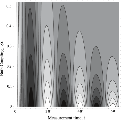
Figure 1: Contour plot of fidelity as a function of coupling $\alpha$, to a zero temperature bath and measurement time $t$. We set $\Delta=1$ and show ten equally spaced contours between $F=0$ $(\alpha=0,t=\pi)$ and $F=1$ $(\alpha=0,t=2\pi n)$. Each shaded band corresponds to an interval of 10%, for example, the white regions correspond to a fidelity of $90\leq F\leq 100\%$, centered around multiples of $\tau$, the uppermost large grey region corresponds to $40\leq F\leq 50\%$ while the black regions correspond to $0\leq F\leq 10\%$.

We see that to obtain high fidelity, we perform the measurements at times given by multiples of $\tau$. In the large $t$ limit the output state decoheres to the maximally mixed state $\frac{1}{2}I$, which reflects a return to the pure cluster state. We also note that the evolution of the encoded quantum information between time $0$ and time $t_{0}$ is distinct from the evolution between $t_{0}$ and $t_{0}+t$ and we will show that, in general, the latter form of evolution is the typical way in which fidelity is lost. For comparing results here with those obtained in the general decoherence situation, we note that the measurement on qubit 1 produces a Hadamard transformation of the encoded state, and consequently swaps the $x$ and $z$ components of the Bloch vector.

II.4 Optimal Cooling Rate

In any experimental realization of MBQC on a strongly coupled system, there will be a residual thermal coupling to an ambient background (the environment), at temperature $T_{\mbox{\tiny bg}}$. Typically, this environment is warm compared to the relevant energy scale in the system, i.e. $kT_{\mbox{\tiny bg}}\gtrsim\Delta$. The coupling to this background can be reduced, for example by screening the system from thermal noise, but usually it can not be eliminated altogether. The purpose of the cooling bath (at temperature $T_{\mbox{\tiny bath}}$) is to counteract this residual heating effect, by actively cooling the system such that the lattice of spins is prepared in a highly entangled cluster state at an effective temperature $kT\ll\Delta,kT_{\mbox{\tiny bg}}$. However, as described in the previous section, the coupling to this bath also has an unwanted effect, which is to reduce the fidelity of MBQC on the system, by disrupting the state of the system over the course of the computation. A reasonable question to ask, then, is how the fidelity of a calculation varies as the strength of the coupling to the cooling bath is varied.

The effects of a cooling bath plus high-temperature background may be modeled by including separate Lindblad terms for each of the baths in the master equation:

$$\dot{\overline{\rho}}(t)=\sum_{i}i\frac{\Delta}{2}[X_{i},\overline{\rho}(t)]\\ +\sum_{i}\Bigl{(}\alpha_{\mbox{\tiny bath}}{\cal D}[|+\rangle_{i}\langle-|]\overline{\rho}(t)+\beta_{\mbox{\tiny bath}}{\cal D}[|-\rangle_{i}\langle+|]\overline{\rho}(t)\Bigr{)}\\ +\sum_{i}\Bigl{(}\alpha_{\mbox{\tiny bg}}{\cal D}[|+\rangle_{i}\langle-|]\overline{\rho}(t)+\beta_{\mbox{\tiny bg}}{\cal D}[|-\rangle_{i}\langle+|]\overline{\rho}(t)\Bigr{)}\,,$$ (14)

where $\alpha_{\mbox{\tiny bath}}$ and $\beta_{\mbox{\tiny bath}}$ describe the coupling to the cooling bath at temperature $T_{\mbox{\tiny bath}}$, and $\alpha_{\mbox{\tiny bg}}$ and $\beta_{\mbox{\tiny bg}}$ are the corresponding coupling strengths to the background environment at temperature $T_{\mbox{\tiny bg}}$. For simplicity, we assume that the background is very warm compared to the energy gap in the system, $kT_{\mbox{\tiny bg}}\gg\Delta$, and use (6) to deduce that $\alpha_{\mbox{\tiny bath}}=\beta_{\mbox{\tiny bath}}\equiv\gamma$, and also that the cooling bath is at a very low temperature $kT_{\mbox{\tiny bath}}\ll\Delta$, such that $\beta_{\mbox{\tiny bath}}=0$. In this limit, the master equation becomes

$$\dot{\overline{\rho}}(t)=\sum_{i}i\frac{\Delta}{2}[X_{i},\overline{\rho}(t)]+\sum_{i}\alpha_{\mbox{\tiny bath}}{\cal D}[|+\rangle_{i}\langle-|]\overline{\rho}(t)\\ +\gamma\sum_{i}\Bigl{(}{\cal D}[|+\rangle_{i}\langle-|]\overline{\rho}(t)+{\cal D}[|-\rangle_{i}\langle+|]\overline{\rho}(t)\Bigr{)}\,.$$ (15)

(Note that the effect of a non-zero temperature cooling bath can also be described by this master equation by a suitable redefinition of $\alpha_{\mbox{\tiny bath}}$, $\beta_{\mbox{\tiny bath}}$ and $\gamma$).

To understand the effect of cooling on the fidelity of a computation, we consider the three qubit example of Sec. II.3, using the master equation (15). We assume that the system is initially in equilibrium under (15) and that the measurements are performed on qubits 1 and 2 at times $t=0$ and $t=2\pi/\Delta$. Between the measurements the system evolves according to the master equation (15), after which we calculate the fidelity between the actual output state on qubit 3 and the ideal output state. The behaviour of the fidelity as a function of the coupling $\alpha_{\mbox{\tiny bath}}$, for various values of $\gamma$, is shown in Fig. 2.

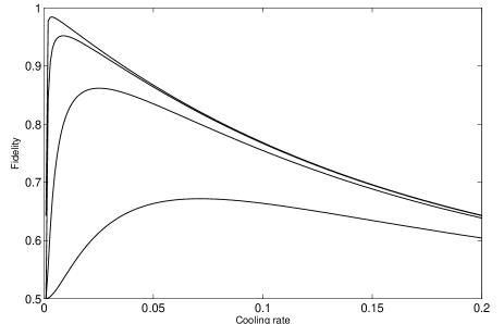
Figure 2: Fidelity as a function of the cooling constant $\alpha_{\mbox{\tiny bath}}$ for couplings to the background (from the bottom to the top) $\gamma=10^{-2},10^{-3},10^{-4}$, and $10^{-5}$. For each there is an optimal cooling rate that maximizes the fidelity.

From Fig.  2 it can be seen that, for large $\alpha_{\mbox{\tiny bath}}$, there is a high loss in fidelity due to rapid dynamics in between the measurement steps, that try to bring the system back to equilibrium. At the other extreme, for a weak coupling to the cooling bath $\alpha_{\mbox{\tiny bath}}\to 0$, the initial state of the system is highly mixed, due to the coupling to the warm background, and so the fidelity is also reduced. There is consequently a trade-off in terms of cooling strength, between counteracting the heating effects of the background and reducing errors due to dynamics between measurements for MBQC on the system. Thus given any ambient background there is an optimal coupling of the system to the cooling bath. Provided the coupling to this cooling bath is under the control of the experimentalist, the optimal coupling should be selected in order to maximise the fidelity of computations.

Note that the two Lindblad terms in (15) can be absorbed into a single term, such that the effect of the two baths is the same as coupling to a single bath with $\alpha=\alpha_{\mbox{\tiny bath}}+\gamma$ and $\beta=\gamma$, so that using (6), the effective temperature of the bath is given by $kT=\Delta/\log(1+\alpha_{\mbox{\tiny bath}}/\gamma)$. In the subsequent sections we treat the system as if it were coupled to a single bath parameterized by $\alpha$ and $\beta$.

III General Decoherence in MBQC

For our simple $X$-rotation gate on a 3 qubit state, we found that the loss in fidelity of the encoded qubit takes on a particularly simple form. In this section, we generalize this result for an arbitrary sequence of measurements in a MBQC scheme, performed at the multiples of the natural timescale $\tau$. Within a general MBQC scheme on a $d$-dimensional lattice, one dimension is identified as “time” and a $(d-1)$-dimensional logical state evolves through the lattice via measurements. We show that the decoherence of this logical state as MBQC proceeds along the time direction coupled via $H_{I}$ to a bath at a given temperature is described by a single quantum operation, acting on the logical state, producing anisotropic decoherence towards the maximally mixed state. The importance of this result is that the error model for the logical qubit is Markovian when we restrict to measurements at multiples of $\tau$ on the cluster state. This error model in turn allows for the application of standard fault-tolerant thresholds.

III.1 One-dimensional lattice

We begin by considering single-qubit unitaries through MBQC on one-dimensional lattices, and will consider the general case in the next section. On a line, with qubits labeled sequentially left to right, consider the situation of already having performed $N-1$ projective measurements after a time $(N-1)\tau$, where $\tau=2\pi/\Delta$ is the natural measurement time. Consequently, the qubit at site $N-1$ is in a pure state, while the qubits $i<N-1$ are partially entangled having evolved back towards the cluster state under the full Hamiltonian for the spin-lattice system coupled to the thermal bath. The qubits $i>N-1$ are in an entangled state and are still awaiting measurement.

We map the qubits $N,N+1,N+2,\cdots$ to a system of unentangled qubits by applying the unitary

$$V_{N}=\prod_{i>N}U_{i-1,i}\,,$$ (16)

where $U_{i-1,i}$ is the controlled-$Z$ unitary between qubit $i-1$ and qubit $i$. This map transforms the Hamiltonian $H_{\mbox{\tiny tot}}\rightarrow H^{\prime}_{\mbox{\tiny tot}}=V_{N}H_{\mbox{\tiny tot}}V_{N}^{\dagger}$ such that qubits $i>N-1$ are uncoupled, and more importantly localizes the logical state to qubit $N$,

The dynamics of the original state is determined by mapping under $V_{N}$, evolving under $H^{\prime}_{\mbox{\tiny tot}}$ and then mapping back with $V_{N}^{\dagger}$. However, because the qubits at sites $i>N$ are assumed to be in equilibrium, they are static under the dynamics and may be ignored, and so we only have to consider the dynamics of the measured qubits together with the logical state at qubit $N$. The logical state, localized at site $N$, decoheres during the time interval $(N-1)\tau$ to $N\tau$ under $H^{\prime}$, where the qubit interacts with site $N-1$ through the cluster Hamiltonian term $-\frac{\Delta}{2}Z_{N-1}X_{N}$, and with the bath through the $\sum_{j}\lambda_{Nj}Z_{N}q_{Nj}$.

The state of the measured qubits and qubit $N$ evolves according to the map ${\cal E}^{\mbox{\tiny tot}}_{\tau}(\rho)=\sum_{I}W_{I,\tau}\rho W_{I,\tau}^{\dagger}$, where the Kraus operators $W_{I}$ for the entire system can be expressed in terms of the Kraus operators $M_{i}$ of Eq. (II.2) as

$$W_{I=\{i_{1},\dots,i_{N}\},\tau}=U(M_{i_{1},\tau}\otimes M_{i_{2},\tau}\otimes\cdots\otimes M_{i_{N},\tau})U^{\dagger}$$ (17)

and where $U$ is the product of all the controlled-$Z$ unitaries for bonds to the left of site $N$.

The evolution has the effect of partially entangling the logical state at $N$ with the other qubits. The input state for the $N^{\mbox{\tiny th}}$ projective measurement is then

$$\mbox{Tr}_{1,\dots,N-1}[{\cal E}^{\mbox{\tiny tot}}_{\tau}(\rho)]=\frac{1}{2}(I+\vec{r}_{N\tau}\cdot\vec{\sigma})\,,$$ (18)

and we obtain the components of its Bloch vector $\vec{r}_{N\tau}$ via $\vec{r}_{N\tau}=\mbox{Tr}[\vec{\sigma}{\cal E}^{\mbox{\tiny tot}}_{\tau}(\rho)]$. Consequently, we can determine the equations of motion for this vector as a function of time from the master equation.

For simplicity, we go to the interaction picture, with $\rho_{I}(t)=\exp[-iH_{c}t]\rho(t)\exp[iH_{c}t]$ and obtain the equations

$$\partial_{t}\langle X_{N}(t)\rangle_{I} =(\alpha-\beta)\langle Z_{N-1}(t)\rangle_{I}-\frac{3}{2}(\alpha+\beta)\langle X_{N}(t)\rangle_{I}$$

$$\partial_{t}\langle Y_{N}(t)\rangle_{I} =-(\alpha+\beta)\langle Y_{N}(t)\rangle_{I}$$

$$\partial_{t}\langle Z_{N}(t)\rangle_{I} =-\frac{1}{2}(\alpha+\beta)\langle Z_{N}(t)\rangle_{I}\,,$$ (19)

where $\langle A(t)\rangle_{I}=\mbox{Tr}[\rho_{I}(t)A]$ for any observable $A$ and $\alpha$ and $\beta$ the temperature dependent coupling parameters as in (4). The equation for the $Z$ component holds for any site $s$ and so $\langle Z_{s}(t)\rangle_{I}=z_{s}\exp[-\frac{1}{2}(\alpha+\beta)t]$. Now all computational measurements in MBQC on the cluster take place in the $X$-$Y$ plane, and so $\langle Z_{s}(t)\rangle=0$ for all $s<N$ and for all time $t$ after site $s$ has been measured.

The components of the logical state in the interaction picture then evolve as

$$\langle X_{N}(t)\rangle_{I} =x_{N}\exp[-\frac{3}{2}(\alpha+\beta)t]\,,$$

$$\langle Y_{N}(t)\rangle_{I} =y_{N}\exp[-(\alpha+\beta)t]\,,$$

$$\langle Z_{N}(t)\rangle_{I} =z_{N}\exp[-\frac{1}{2}(\alpha+\beta)t]\,.$$ (20)

However, at times $t=n\tau$, we have $\rho_{I}(t)=\rho(t)$, and so for these times the decoherence to the maximally mixed state is deduced from the interaction picture results, and agrees with the explicit example of the 3 qubit system in Sec. II.3.

The result of this analysis is that the MBQC scheme along the line of qubits with a free Hamiltonian and in contact with a bath at a finite temperature can be described in simple terms for any sequence of measurements on the logical state at times which are multiples of $\tau$, using a fixed Markovian noise operator $\mathcal{F}$. For a sequence of measurements $\{\phi_{1},\phi_{2},\dots\phi_{N}\}$ in the $X$-$Y$ plane labelled at each site by an angle $\phi$ from the $X$ axis and with outcomes $\{s_{1},s_{2},\dots,s_{N}\}$, the single qubit logical state is processed as

$$\psi_{\mbox{\tiny in}} \rightarrow[Z^{s_{1}}X(\phi_{1})H][\psi_{\mbox{\tiny in}}]\rightarrow{\cal F}[[Z^{s_{1}}X(\phi_{1})H][\psi_{\mbox{\tiny in}}]]\rightarrow$$

$$\rightarrow[Z^{s_{2}}X(\phi_{2})H][{\cal F}[[Z^{s_{1}}X(\phi_{1})H][\psi_{\mbox{\tiny in}}]]]\rightarrow$$

$$\rightarrow{\cal F}[[Z^{s_{2}}X(\phi_{2})H][{\cal F}[[Z^{s_{1}}X(\phi_{1})H][\psi_{\mbox{\tiny in}}]]]]\rightarrow\cdots\,,$$ (21)

where for any $A$ we denote $[A][\rho]=A\rho A^{\dagger}$, $H=|+\rangle\langle 0|+|-\rangle\langle 1|$, $X(\phi)=\exp(-i\frac{\phi}{2}X)$, and ${\cal F}[\rho]$ is the quantum operation given by

$${\cal F}[\rho]=p_{1}\rho+p_{2}X\rho X+p_{3}Y\rho Y+p_{4}Z\rho Z\,,$$ (22)

with

$$p_{1} =\frac{1}{4}(1+w)(1+w^{2})\hskip 14.22636ptp_{2}=\frac{1}{4}(1-w)(1-w^{2})$$

$$p_{3} =\frac{1}{4}(1-w)(1+w^{2})\hskip 14.22636ptp_{4}=\frac{1}{4}(1+w)(1-w^{2})$$ (23)

and $w=\exp[-(\alpha+\beta)t/2]$.

It is also clear from this analysis why in the case of an arbitrary $X$ rotation performed with three qubits, that the first evolution is slightly different from the second one: before the first measurement there are no qubits to the left of the first site to affect the logical state, while the qubits to the right are already in their equilibrium state, and so the evolution of the state is localized to the first site.

III.2 General lattices

The analysis of the last section can be extended to higher-dimensional lattices. For example, if upon localization to a site $s$ using an analogous unitary to $V_{N}$, the single qubit logical state has $k$ neighbouring sites, labeled $1,2,3,\dots,k$, then (III.1) generalizes to

$$\partial_{t}\langle X_{s}(t)\rangle_{I} =(\alpha-\beta)\langle Z_{1}\cdots Z_{k}(t)\rangle_{I}$$

$$\quad-\frac{k+2}{2}(\alpha+\beta)\langle X_{s}(t)\rangle_{I}$$

$$\partial_{t}\langle Y_{s}(t)\rangle_{I} =-\frac{k+1}{2}(\alpha+\beta)\langle Y_{s}(t)\rangle_{I}$$

$$\partial_{t}\langle Z_{s}(t)\rangle_{I} =-\frac{1}{2}(\alpha+\beta)\langle Z_{s}(t)\rangle_{I}$$

$$\partial_{t}\langle Z_{1}\cdots Z_{k}(t)\rangle_{I} =-\frac{k}{2}(\alpha+\beta)\langle Z_{1}\cdots Z_{k}(t)\rangle_{I}\,.$$ (24)

For general MBQC on for example the 2D or 3D lattice, we assume that the adaptive measurements are performed in steps, with a time interval $\tau$ before the next round of measurements. Each round of measurements is composed of a set of $Z$ measurements to eliminate qubits from the lattice and a set of measurements in the $X$-$Y$ plane to propagate correlations and to perform the desired computational transformations.

After $N-1$ such measurement steps, we may formally disentangle the qubits to be measured at steps $N,N+1,N+2,\dots$ and transform to a system where the logical state is localized to a set of qubits, which we denote $\mathcal{Q}_{N}$. Once again, the qubits to measured at stages $N+1,N+2,\dots$ are in their equilibrium states and can be ignored for the timestep. The reduced state for the logical state after a time $\tau$ is determined from terms of the form $\langle M\rangle_{I}$, where $M$ is a product of Pauli operators on $\mathcal{Q}_{N}$ and its surrounding qubits.

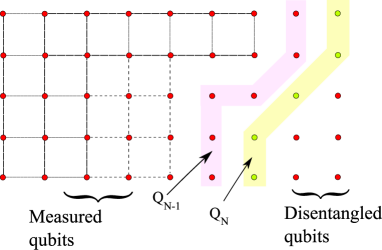
Figure 3: Schematic diagram for the localization of the logical state to the qubits $\mathcal{Q}_{N}$ after $N-1$ timesteps. The qubits to the right of $\mathcal{Q}_{N}$ are disentangled with a unitary $V_{N}$, while those to the left have already been measured. The qubits $\mathcal{Q}_{N-1}$ are in a pure product state, having just been measured.

A site $i$ on the lattice contributes to the equation of motion of a general observable $M$ according to the following rule: it contributes $-\frac{(\alpha+\beta)}{2}\langle M\rangle_{I}$ if either $[M,Z_{i}]=\{M,K_{i}\}=0$ or if $\{M,Z_{i}\}=\{M,K_{i}\}=0$; it contributes $-(\alpha+\beta)\langle M\rangle_{I}+(\alpha-\beta)\langle MK_{i}\rangle_{I}$ if $\{M,Z_{i}\}=[M,K_{i}]=0$; and zero otherwise. Consequently, awkward terms can arise when $M$ contains an $X$ observable. These terms couple the equations of motion for observables on $\mathcal{Q}_{N}$ with observables on $\mathcal{Q}_{N}$ plus its neighbours, however for MBQC on the cluster state these equations decouple, from the following argument.

For an observable $M$ on $\mathcal{Q}_{N}$ containing $m$ $X_{i}$ observables, its equation of motion will only have terms of the form $\langle M\rangle_{I}$ and $\langle MK_{i}\rangle_{I}$. However $MK_{i}$ is an observable with $(m-1)$ $X$’s on $\mathcal{Q}_{N}$ and a number of $Z$’s in $\mathcal{Q}_{N-1}$, the set of qubits that have just been measured. If we iterate and obtain the full set of coupled equations that determine $\langle MK_{i}\rangle_{I}$ we arrive at a dependence on observables without any $X$ observables and with at least one $Z_{s}$ on site $s$ in $\mathcal{Q}_{N-1}$. The equation of motion for such an observable $M^{\prime}$ is of the form $\partial_{t}\langle M^{\prime}\rangle_{I}=-p(\alpha+\beta)/2\langle M^{\prime}\rangle_{I}$ for some integer $p$. Furthermore, if $s$ was measured in the $X$-$Y$ plane then initially $\langle M^{\prime}\rangle_{I}=0$ and so will remain zero for the whole time interval. Retracing the chain of coupled equations we find that each problematic term of the form $\langle MK_{i}\rangle_{I}$ vanishes for $t\geq 0$ and the equations of motion for the observables on $\mathcal{Q}_{N}$ are decoupled provided each qubit in $\mathcal{Q}_{N}$ has at least one neighbour in $\mathcal{Q}_{N-1}$ that was measured in the $X$-$Y$ plane.

The expectation of an observable $M$ on $\mathcal{Q}_{N}$ will evolve as $\langle M\rangle_{I}=M_{0}e^{-q(\alpha+\beta)t/2}$ for some integer $q$, and for Pauli observables $M_{1},M_{2}\dots,M_{k}$ on sites $1,2,\dots,k$ we have that $|\langle M_{1}\cdots M_{k}(t)\rangle_{I}|\geq|\langle M_{1}(t)\rangle_{I}|\cdots|\langle M_{k}(t)\rangle_{I}|$, with equality coming when the sites do not share any neighbours.

III.3 Fault tolerance

With a simple Markovian description of the errors present in our scheme, we can consider fault-tolerant MBQC. There are two sources of errors in the dynamical setting that we are considering. First, the equilibrium state for the system is at a non-zero temperature, and so there are preparation errors due to an imperfectly prepared cluster state. Second, errors occur due to the dynamics between measurements, and can be viewed as storage errors on the qubits for a given timestep. For sufficiently low rates, MBQC on a 3D lattice has been shown to be fault-tolerant for both of these sources of errors Rau06 ; Rau07 . If the state distillation protocol of Ref.  Rau07 is used, the error threshold is set by the bulk topological part of the error correction scheme, which in turn can be related to a phase transition in the classical random plaquette gauge model  Wang02 .

Our initial state is a thermal state, static under the dynamics, prepared by cooling with the bath. Such a thermal cluster state at a temperature $T$ is obtained by applying $Z$ errors to a perfect cluster state with probability $p_{\mbox{\tiny prep}}=(1+\exp(\Delta/(kT)))^{-1}$.

For the cubic lattice model, the dynamics in between measurement steps produce an error channel on the individual qubits no worse than a quantum operation of the same form as (22) but with coefficients

$$p_{1} =\frac{1}{4}(1+w)(1+w^{6})\hskip 14.22636ptp_{2}=\frac{1}{4}(1-w)(1-w^{6})$$

$$p_{3} =\frac{1}{4}(1-w)(1+w^{6})\hskip 14.22636ptp_{4}=\frac{1}{4}(1+w)(1-w^{6})\,,$$ (25)

and with $w=e^{-(\alpha+\beta)\tau/2}$. Consequently, the resultant errors for a cubic lattice are no worse than those obtained by application of the local depolarizing channel $T[\rho]=(1-p_{s})\rho+\frac{p_{s}}{3}(X\rho X+Y\rho Y+Z\rho Z)$ with $p_{s}=\frac{1}{4}(1+w)(1-w^{6})$, on each individual qubit.

The combined effect of these two errors leads to independent errors on each qubit in the lattice with effective parameter $q=p_{\mbox{\tiny prep}}+\frac{2}{3}p_{s}$ (c.f.  Rau06 ). The threshold for such errors is given by $q<0.0293$  Wang02 . Thus, if errors due to the dynamics can be neglected, i.e. when $p_{s}\to 0$, the error threshold for preparation errors corresponds to a temperature bound of $T\sim 0.28\Delta$. Conversely, if errors due to preparation can be neglected, $p_{\mbox{\tiny prep}}\to 0$, the error threshold corresponds to a threshold for the environmental couplings of $(\alpha+\beta)/\Delta\sim 4.6\times 10^{-3}$.

If this environment consists of a infinite temperature background parametrized by $\gamma$ and a zero-temperature cooling bath parametrized by $\alpha_{\rm bath}$ as in Sec. II.4, the parameter $q$ is a function of these two parameters. The constraint $q(\alpha_{\rm bath},\gamma)=0.0293$ defines the threshold value of $\gamma$ implicitly in terms of $\alpha_{\rm bath}$. We may then maximize this $\gamma$ over the bath couplings and deduce an overall threshold of $\gamma/\Delta\sim 3.4\times 10^{-5}$ for the coupling to the environment provided that the cooling rate for the bath is set at a “Goldilocks value” of $\alpha_{\rm bath}/\Delta\sim 2.26\times 10^{-3}$. For this cooling rate the system is not so hot that large preparation errors destroy entanglement, and it is not so cold that large storage errors erase the logical state. That is, if the coupling to the background environment $\gamma$ is below this threshold, it is possible to devise a cooling bath that allows for fault-tolerant MBQC.

IV Discussion

When the ground state of a physical system provides a resource state for MBQC we must necessarily take into account the system’s dynamics. As we have discussed there are several sources of complication compared with MBQC on a static resource. While we may prepare the system very close to its ground state, any measurements we then perform on it will produce excitations and for a general adaptive measurement scheme, involving classical feed-forward, the resultant dynamics between measurements will perturb the state and affect the computation.

For the simple, dispersionless Hamiltonian (1) describing a lattice of spins we showed that measurements should be performed at a characteristic clock speed $2\pi/\Delta$ defined via the energy gap $\Delta$. However, the presence of environmental interactions further complicates matters. For the environment, we considered both ambient background effects and also the effects of a thermal bath used to prepare and maintain the lattice system. We found that an optimal cooling exists, which is a trade-off between adequate shielding of the system from a hot background and providing slow dynamics that allow adaptive measurements. Furthermore, the loss in fidelity due to this dynamics is conveniently described in terms of a single quantum operation (22) that acts on the logical state.

The importance of our results is that under certain conditions, the environment produces Markovian errors on the logical state and is thus amenable to error-correction. Our results are general and do not depend on the type of lattice or its dimensionality. In the particular case of a cubic lattice we may invoke fault-tolerance results for MBQC in the presence of local independent depolarizing errors to obtain a threshold of $T\sim 0.28\Delta$ for the temperature of the prepared state when dynamics may be neglected, and a threshold of $(\alpha+\beta)/\Delta\sim 4.6\times 10^{-3}$ for the ratio of environmental couplings to energy gap when the storage errors dominate. In addition, we obtained a threshold of $\gamma/\Delta\sim 3.4\times 10^{-5}$ for the coupling to a high temperature environment provided there is a zero-temperature cooling bath with coupling $\alpha_{\rm bath}/\Delta\sim 2.26\times 10^{-3}$ to the lattice system.

Several issues remain that deserve investigation. For example, we have not discussed possible imperfections in the Hamiltonian or measurement errors, both of which would modify the above thresholds. Furthermore, the free Hamiltonian behaviour suggests the obvious strategy of performing all measurements at or near the clock cycles of $\tau=2\pi/\Delta$. However more complicated measurement strategies may exist that produce high fidelities in the presence of a fixed cooling.

While the above formalism may be adapted to different settings or more particular questions, another key outstanding issue is the effect of finite-time measurements in which the measurements themselves are not instantaneous but are spread over some small finite interval of time. Such a situation requires a more elaborate analysis than the one presented here, especially when the measurement time becomes comparable with the clock cycle time $\tau$.

- (1) R. Raussendorf and H. J. Briegel, Phys. Rev. Lett. 86, 5188 (2001).
- (2) R. Raussendorf, D. E. Browne and H.J. Briegel, Phys. Rev. A68, 022312 (2003).
- (3) P. Treutlein et al., Fortschr. Phys. 54, 702 (2006).
- (4) D. E. Browne and T. Rudolph, Phys. Rev. Lett. 95, 010501 (2005).
- (5) P. Walther et al., Nature (London)434, 169 (2005).
- (6) R. Raussendorf, S. Bravyi, J. Harrington, Phys. Rev. A71, 062313 (2005).
- (7) S. D. Bartlett and T. Rudolph, Phys. Rev. A74, 040302(R) (2006); T. Griffin and S. D. Bartlett, Phys. Rev. A78, 062306 (2008).
- (8) A. C. Doherty and S. D. Bartlett, Phys. Rev. Lett. 103, 020506 (2009).
- (9) S. D. Barrett, S. D. Bartlett, A. C. Doherty, D. Jennings, T. Rudolph, arXiv:0807.4797.
- (10) G. K. Brennen and A. Miyake, Phys. Rev. Lett. 101, 010502 (2008).
- (11) S. O. Skrøvseth and S. D. Bartlett, Phys. Rev. A80, 022316 (2009).
- (12) D. Gross, J. Eisert, N. Schuch, D. Perez-Garcia, Phys. Rev. A76, 052315 (2007).
- (13) D. Gross, S. T. Flammia, and J. Eisert, Phys. Rev. Lett. 102, 190501 (2009).
- (14) M. J. Bremner, C. Mora, and A. Winter, Phys. Rev. Lett. 102, 190502 (2009).
- (15) M. A. Nielsen and I. L. Chuang, Quantum Computation and Quantum Information, (Cambridge University Press, Cambridge, 2000).
- (16) F. Verstraete, M. M. Wolf, and J. I. Cirac, arXiv:0803.1447.
- (17) D. F. Walls and G. J. Milburn. Quantum Optics (Springer, 1995).
- (18) M. Hein, W. Dür, J. Eisert, R. Raussendorf, M. Van den Nest, and H.-J. Briegel, arXiv:quant-ph/0602096v1.
- (19) R. Raussendorf, J. Harrington, and K. Goyal, Ann. Phys. 321, 2242 (2006).
- (20) R. Raussendorf, J. Harrington, and K. Goyal, New J. Phys. 9, 199 (2007).
- (21) C. Wang, J. Harrington, and J. Preskill, Ann. Phys. 303, 31 (2003).