Algorithmic design of self-assembling structures

Abstract

We study inverse statistical mechanics: how can one design a potential function so as to produce a specified ground state? In this paper, we show that unexpectedly simple potential functions suffice for certain symmetrical configurations, and we apply techniques from coding and information theory to provide mathematical proof that the ground state has been achieved. These potential functions are required to be decreasing and convex, which rules out the use of potential wells. Furthermore, we give an algorithm for constructing a potential function with a desired ground state.

I Introduction

How can one engineer conditions under which a desired structure will spontaneously self-assemble from simpler components? This inverse problem arises naturally in many fields, such as chemistry, materials science, biotechnology, or nanotechnology (see for example ref. To and the references cited therein). A full solution remains distant, but in this paper we develop connections with coding and information theory, and we apply these connections to give a detailed mathematical analysis of several fundamental cases.

Our work is inspired by a series of papers by Rechtsman, Stillinger, and Torquato, in which they design potential functions that can produce a honeycomb RST1 , square RST2 , cubic RST3 , or diamond RST4 lattice. In this paper, we analyze finite analogues of these structures, and we show similar results for much simpler classes of potential functions.

For an initial example, suppose $20$ identical point particles are confined to the surface of a unit sphere (in the spirit of the Thomson problem of how classical electrons arrange themselves on a spherical shell). We wish them to form a regular dodecahedron with $12$ pentagonal facets.

Suppose the only flexibility we have in designing the system is that we can specify an isotropic pair potential $V$ between the points. In other words, the potential energy $E_{V}(\mathcal{C})$ of a configuration (i.e., set of points) $\mathcal{C}$ is

$$E_{V}(\mathcal{C})=\frac{1}{2}\sum_{x,y\in\mathcal{C},\,x\neq y}V\big{(}|x-y|\big{)}.$$ (1)

In static equilibrium, the point configuration will assume a form that at least locally minimizes $E_{V}(\mathcal{C})$. Can we arrange for the energy-minimizing configuration to be a dodecahedron? Furthermore, can we arrange for it to have a large basin of attraction under natural processes such as gradient descent? If so, then we can truly say that the dodecahedron automatically self-assembles out of randomly arranged points when the proper potential function is imposed.

If we could choose $V$ arbitrarily, then it would certainly be possible to make the dodecahedron the global minimum for energy by using potential wells, as in the blue graph in Fig. 1. By contrast, this cannot be done with familiar potential functions, such as inverse power laws, because the dodecahedron’s pentagonal facets are highly unstable and prone to collapse into a triangulation.

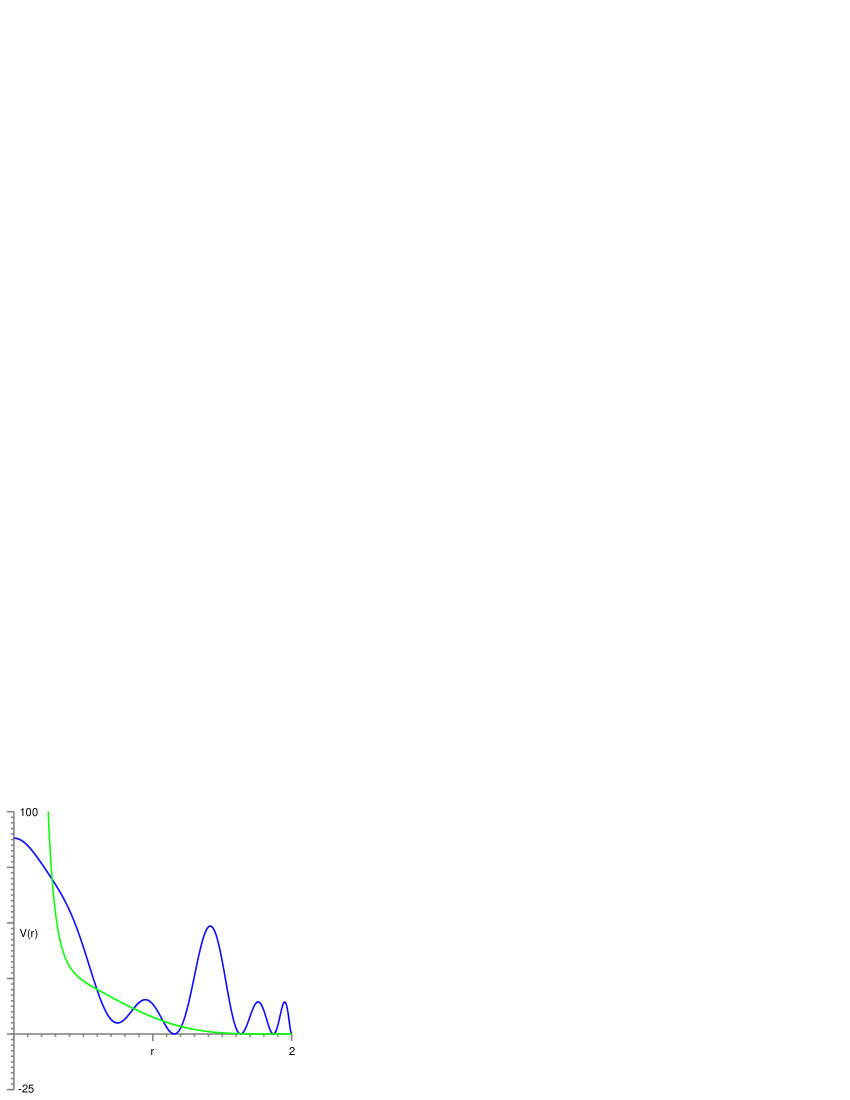
Figure 1: Two potential functions under which the regular dodecahedron minimizes energy: the blue one uses potential wells, while the green one is convex and decreasing.

Unfortunately, the potential function shown in the blue graph in Fig. 1 is quite elaborate. Actually implementing precisely specified potential wells in a physical system would be an enormous challenge. Instead, one might ask for a simpler potential function, for example one that is decreasing and convex (corresponding to a repulsive, decaying force).

Figure 2: The paths of points converging to the regular dodecahedron under the green potential function from Fig. 1. Only the front half of the sphere is shown.

In fact, $V$ can be chosen to be both decreasing and convex. The green graph in Fig. 1 shows such a potential function, which is described and analyzed in Theorem 4. We prove that the regular dodecahedron is the unique ground state for this system. We have been unable to prove anything about the basin of attraction, but computer simulations indicate that it is large (we performed $1200$ independent trials using random starting configurations, and all but $6$ converged to the dodecahedron). For example, Fig. 2 shows the paths of the particles in a typical case, with the passage of time indicated by the transition from yellow to red.

Our approach to this problem makes extensive use of linear programming. This enables us to give a probabilistic algorithm for inverse statistical mechanics. Using it, we construct simple potential functions with counterintuitive ground states. These states are analogues of those studied in refs. RST1 ; RST2 ; RST3 ; RST4 , but we use much simpler potential functions. Finally, we make use of the linear programming bounds from coding theory to give rigorous mathematical proofs for some of our assertions. These bounds allow us to prove that the desired configurations are the true ground states of our potential functions. By contrast, previous results in this area were purely experimental and could not be rigorously analyzed.

I.1 Assumptions and Model

To arrive at a tractable problem, we make four fundamental assumptions. First, we will deal with only finitely many particles confined to a bounded region of space. This is not an important restriction in itself, because periodic boundary conditions could create an effectively infinite number of particles.

Second, we will use classical physics, rather than quantum mechanics. Our ideas are not intrinsically classical, but computational necessity forces our hand. Quantum systems are difficult to simulate classically (otherwise the field of quantum computing would not exist), and there is little point in attempting to design systems computationally when we cannot even simulate them. Fortunately, classical approximations are often of real-world as well as theoretical value. For example, they are excellent models for soft matter systems such as polymers and colloids L ; RSS .

Third, we restrict our attention to a limited class of potential functions, namely isotropic pair potentials. These potentials depend only on the pairwise distances between the particles, with no directionality and no three-particle interactions; they are the simplest potential functions worthy of analysis. For example, the classical electric potential is of this sort. We expect that our methods will prove useful in more complex cases, but isotropic pair potentials have received the most attention in the literature and already present many challenges.

Finally, we assume all the particles are identical. This assumption plays no algorithmic role and is made purely for the sake of convenience. The prettiest structures are often the most symmetrical, and using identical particles facilitates such symmetry.

We must still specify the ambient space for the particles. Three choices are particularly natural: we could study finite clusters of particles in Euclidean space, configurations in a flat torus (i.e., a region in space with periodic boundary conditions, so the number of particles is effectively infinite), or configurations on a sphere. Our algorithms apply to all three cases, but in this paper we will focus on spherical configurations. They are in many ways the most symmetrical case, and they are commonly analyzed, for example in Thomson’s problem of arranging classical electrons on a sphere.

Thus, we will use the following model. Suppose we have $N$ identical point particles confined to the surface of the unit sphere $S^{n-1}=\{x\in{\mathbb{R}}^{n}:|x|=1\}$ in $n$-dimensional Euclidean space ${\mathbb{R}}^{n}$. (We choose to work in units in which the radius is $1$, but of course any other radius can be achieved by a simple rescaling.) We use a potential function $V\colon(0,2]\to{\mathbb{R}}$, for which we define the energy of a configuration $\mathcal{C}\subset S^{n-1}$ as in Eq. (1). We define $V$ only on $(0,2]$ because no other distances occur between distinct points on the unit sphere.

Note that we have formulated the problem in an arbitrary number $n$ of dimensions. It might seem that $n=3$ would be the most relevant for the real world, but $n=4$ is also a contender, because the surface of the unit sphere in ${\mathbb{R}}^{4}$ is itself a three-dimensional manifold (merely embedded in four dimensions). We can think of $S^{3}$ as an idealized model of a curved three-dimensional space. This curvature is important for the problem of “geometrical frustration” SM : many beautiful local configurations of particles do not extend to global configurations, but once the ambient space is given a small amount of curvature they piece together cleanly. As the curvature tends to zero (equivalently, as the radius of the sphere or the number of particles tends to infinity), we recover the Euclidean behavior. Although this may sound like an abstract trick, it sometimes provides a strikingly appropriate model for a real-world phenomenon; see, for example, figure 2.6 in ref. SM , which compares the radial distribution function obtained by X-ray diffraction on amorphous iron to that from a regular polytope in $S^{3}$ and finds an excellent match between the peaks.

The case of the ordinary sphere $S^{2}$ in ${\mathbb{R}}^{3}$ is also more closely connected to actual applications that it might at first appear. One scenario is a Pickering emulsion, in which colloidal particles adsorb onto small droplets in the emulsion. The particles are essentially confined to the surface of the sphere and can interact with each other, for example, via a screened Coulomb potential or by more elaborate potentials. This approach has in fact been used in practice to fabricate colloidosomes DHNMBW . See also the review article BG , in particular section 1.2, and the references cited therein for more examples of physics on curved, two-dimensional surfaces, such as amphiphilic membranes or viral capsids.

I.2 Questions and Problems

From the static perspective, we wish to understand what the ground state is (i.e., which configuration minimizes energy) and what other local minima exist. From the dynamic perspective, we wish to understand the movement of particles and the basins of attraction of the local minima for energy. There are several fundamental questions:

1. Given a configuration $\mathcal{C}$, can one choose an isotropic pair potential $V$ under which $\mathcal{C}$ is the unique ground state for $|\mathcal{C}|$ points?

2. How simple can $V$ be? Can it be decreasing? Convex?

3. How large can the basin of attraction be made?

In this paper, we give a complete answer to the first question, giving necessary and sufficient conditions for such a potential to exist. The second question is more subtle, but we rigorously answer it for several important cases. In particular, we show that one can often use remarkably simple potential functions. The third question is the most subtle of all, and there is little hope of providing rigorous proofs; instead, experimental evidence must suffice.

The second question is particularly relevant for experimental work, for example with colloids, because only a limited range of potentials can be manipulated in the lab. Inverse statistical mechanics with simple potential functions was therefore raised as a challenge for future work in ref. To .

We will focus on four especially noteworthy structures:

1. The $8$ vertices of a cube, with $6$ square facets.

2. The $20$ vertices of a regular dodecahedron, with $12$ pentagonal facets.

3. The $16$ vertices of a hypercube in four dimensions, with $8$ cubic facets (see Fig. 3).

4. The $600$ vertices of a regular $120$-cell in four dimensions, with $120$ dodecahedral facets (see Fig. 4).

The latter two configurations exist in four dimensions, but as discussed above the sphere containing them is a three-dimensional space, so they are intrinsically three-dimensional.

Figure 3: The hypercube, drawn in four-point perspective.

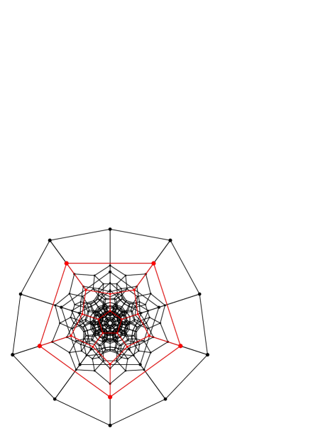
Figure 4: The Schlegel diagram for the regular $120$-cell (with a dodecahedral facet in red).

These configurations are important test cases, because they are elegant and symmetrical yet at the same time not at all easy to build. The problem is that their facets are too large, which makes them highly unstable. Under ordinary potential functions, such as inverse power laws, these configurations are never even local minima, let alone global minima. In the case of the cube, one can typically improve it by rotating two opposite facets so they are no longer aligned. That lowers the energy, and indeed the global minimum appears to be the antiprism arrived at via a $45^{\circ}$ rotation (and subsequent adjustment of the edge lengths). It might appear that this process always works, and that the cube can never minimize a convex, decreasing potential function. However, careful calculation shows that this argument is mistaken, and we will exhibit an explicit convex, decreasing potential function for which the cube is provably the unique global minimum.

One reason why the four configurations mentioned above are interesting is that they are spherical analogues of the honeycomb and diamond packings from ${\mathbb{R}}^{2}$ and ${\mathbb{R}}^{3}$, respectively. In each of our four cases, the nearest neighbors of any point form the vertices of a regular spherical simplex. They have the smallest possible coordination numbers that can occur in locally jammed packings (see, for example, ref. DTSC ).

II Potential wells

Suppose $\mathcal{C}$ is a configuration in $S^{n-1}$. The obvious way to build $\mathcal{C}$ is to use deep potential wells (i.e., local minima in $V$) corresponding to the distances between points in $\mathcal{C}$, so that configurations that use only those distances are energetically favored. This method produces complicated potential functions, which may be difficult to produce in the real world, but it is systematic and straightforward. In this section we rigorously analyze the limitations of this method and determine exactly when it works, thereby answering a question raised towards the end of ref. RST1 .

The first limitation is obvious. Define the distance distribution of $\mathcal{C}$ to be the function $d$ such that $d(r)$ is the number of pairs of points in $\mathcal{C}$ at distance $r$. The distance distribution determines the potential energy via

$$E_{V}(\mathcal{C})=\sum_{r}V(r)\,d(r).$$ (2)

Thus, $\mathcal{C}$ cannot possibly be the unique ground state unless it is the only configuration with its distance distribution.

The second limitation is more subtle. The formula (2) shows that $E_{V}$ depends linearly on $d$. If $d$ is a weighted average of the distance distributions of some other configurations, then the energy of $\mathcal{C}$ will be the same weighted average of the other configurations’ energies. In that case, one of those configurations must have energy at least as low as that of $\mathcal{C}$. Call $d$ extremal if it is an extreme point of the convex hull of the space of all distance distributions of $|\mathcal{C}|$-point configurations in $S^{n-1}$ (i.e., it cannot be written as a weighted average of other distance distributions). If $\mathcal{C}$ is the unique ground state for some isotropic pair potential, then $d$ must be extremal.

For an example, consider three-point configurations on the circle $S^{1}$, specified by the angles between the points (the shorter way around the circle). The distance distribution of the configuration with angles $45^{\circ}$, $90^{\circ}$, and $135^{\circ}$ is not extremal, because it is the average of those for the $45^{\circ}$, $45^{\circ}$, $90^{\circ}$ and $90^{\circ}$, $135^{\circ}$, $135^{\circ}$ configurations.

Theorem 1.

If $\mathcal{C}$ is the unique configuration in $S^{n-1}$ with its distance distribution $d$ and $d$ is extremal, then there exists a smooth potential function $V\colon(0,2]\to{\mathbb{R}}$ under which $\mathcal{C}$ is the unique ground state among configurations of $|\mathcal{C}|$ points in $S^{n-1}$.

The analogue of Theorem 1 for finite clusters of particles in Euclidean space is also true, with almost exactly the same proof.

Proof: Because $d$ is extremal, there exists a function $\ell$ defined on the support $\mathop{\textup{supp}}(d)$ of $d$ [i.e., the set of all $r$ such that $d(r)\neq 0$] such that $d$ is the unique minimum of

$$t\mapsto\sum_{r}\ell(r)\,t(r)$$

among $|\mathcal{C}|$-point distance distributions $t$ with $\mathop{\textup{supp}}(t)\subseteq\mathop{\textup{supp}}(d)$. Such a function corresponds to a supporting hyperplane for the convex hull of the distance distributions with support contained in $\mathop{\textup{supp}}(d)$.

For each $\varepsilon>0$, choose any smooth potential function $V_{\varepsilon}$ such that $V_{\varepsilon}(r)=\ell(r)$ for $r\in\mathop{\textup{supp}}(d)$ while

$$V_{\varepsilon}(s)>\sum_{r}\ell(r)\,d(r)$$

whenever $s$ is not within $\varepsilon$ of a point in $\mathop{\textup{supp}}(d)$. This is easily achieved using deep potential wells, and it guarantees that no configuration can minimize energy unless every distance occurring in it is within $\varepsilon$ of a distance occurring in $\mathcal{C}$. Furthermore, when $\varepsilon$ is sufficiently small [specifically, less than half the distance between the closest two points in $\mathop{\textup{supp}}(d)$], choose $V_{\varepsilon}$ so that for each $r\in\mathop{\textup{supp}}(d)$, we have $V(s)>V(r)$ whenever $|s-r|\leq\varepsilon$ and $s\neq r$.

For a given $\varepsilon$, there is no immediate guarantee that $\mathcal{C}$ will be the ground state. However, consider what happens to the ground states under $V_{\varepsilon}$ as $\varepsilon$ tends to $0$. All subsequential limits of their distance distributions must be distance distributions with support in $\mathop{\textup{supp}}(d)$. Because of the choice of $\ell$, the only possibility is that they are all $d$. In other words, as $\varepsilon$ tends to $0$ the distance distributions of all ground states must approach $d$. Because the number of points at each given distance is an integer, it follows that when $\varepsilon$ is sufficiently small, for each $r\in\mathop{\textup{supp}}(d)$, there are exactly $d(r)$ distances in each ground state that are within $\varepsilon$ of $r$. Because $V_{\varepsilon}$ has a strict local minimum at each point in $\mathop{\textup{supp}}(d)$, it follows that it is minimized at $d$ (and only at $d$) when $\varepsilon$ is sufficiently small. The conclusion of the theorem then follows from our assumption that $\mathcal{C}$ is the unique configuration in $S^{n-1}$ with distance distribution $d$. $\Box$

It would be interesting to have a version of Theorem 1 for infinite collections of particles in Euclidean space, but there are technical obstacles. Having infinitely many distances between particles makes the analysis more complicated, and one particular difficulty is what happens if the set of distances has an accumulation point or is even dense (for example in the case of a disordered packing). In such a case there seems to be no simple way to use potential wells, but in fact a continuous function with a fractal structure can have a dense set of strict local minima, and perhaps it could in theory serve as a potential function.

III Simulation-guided optimization

In this section we describe an algorithm for optimizing the potential function to create a specified ground state. Our algorithm is similar to, and inspired by, the zero-temperature optimization procedure introduced in ref. RST2 ; the key difference is that their algorithm is based on a fixed list of competing configurations and uses simulated annealing, whereas ours dynamically updates that list and uses linear programming. (We also omit certain conditions on the phonon spectrum that ensure mechanical stability. In our algorithm, they appear to be implied automatically once the list of competitors is sufficiently large.)

Suppose the allowed potential functions are the linear combinations of a finite set $V_{1},\dots,V_{k}$ of specified functions. In practice, this may model a situation in which only certain potential functions are physically realizable, with relative strengths that can be adjusted within a specified range, while in theory we may choose the basic potential functions so that their linear combinations can approximate any reasonable function arbitrarily closely as $k$ becomes large.

Given a configuration $\mathcal{C}\subset S^{n-1}$, we wish to choose a linear combination

$$V=\lambda_{1}V_{1}+\dots+\lambda_{k}V_{k}$$

so that $\mathcal{C}$ is the global minimum for $E_{V}$. We may also wish to impose other conditions on $V$, such as monotonicity or convexity. We assume that all additional conditions are given by finitely many linear inequalities in the coefficients $\lambda_{1},\dots,\lambda_{k}$. (For conditions such as monotonicity or convexity, which apply over the entire interval $(0,2]$ of distances, we approximate them by imposing these conditions on a large but finite subset of the interval.)

Given a finite set of competitors $\mathcal{C}_{1},\dots,\mathcal{C}_{\ell}$ to $\mathcal{C}$, we can choose the coefficients by solving a linear program. Specifically, we add an additional variable $\Delta$ and impose the constraints

$$E_{V}(\mathcal{C}_{i})\geq E_{V}(\mathcal{C})+\Delta$$

for $1\leq i\leq\ell$, in addition to any additional constraints (as in the previous paragraph). We then choose $\lambda_{1},\dots,\lambda_{k}$ and $\Delta$ so as to maximize $\Delta$ subject to these constraints. Because this maximization problem is a linear program, its solution is easily found.

If the coefficients can be chosen so that $\mathcal{C}$ is the global minimum, then $\Delta$ will be positive and this procedure will produce a potential function for which $\mathcal{C}$ has energy less than each of $\mathcal{C}_{1},\dots,\mathcal{C}_{\ell}$. The difficulty is how to choose these competitors. In some cases, it is easy to guess the best choices: for example, the natural competitors to a cube are the square antiprisms. In others, it is far from easy. Which configurations compete with the regular $120$-cell in $S^{3}$?

Our simulation-guided algorithm iteratively builds a list of competitors and an improved potential function. We start with any choice of coefficients, say $\lambda_{1}=1$ and $\lambda_{2}=\dots=\lambda_{k}=0$, and the empty list of competitors. We then choose $|\mathcal{C}|$ random points on $S^{n-1}$ and minimize energy by gradient descent to produce a competitor to $\mathcal{C}$, which we add to the list (if it is different from $\mathcal{C}$) and use to update the choice of coefficients. This alternation between gradient descent and linear programming continues until either we are satisfied that $\mathcal{C}$ is the global minimum of the potential function, or we find a list of competitors for which linear programming shows that $\Delta$ must be negative (in which case no choice of coefficients makes $\mathcal{C}$ the ground state).

This procedure is only a heuristic algorithm. When $\Delta$ is negative, it proves that $\mathcal{C}$ cannot be the ground state (using linear combinations of $V_{1},\dots,V_{k}$ satisfying the desired constraints), but otherwise nothing is proved. As the number of iterations grows large, the algorithm is almost certain to make $\mathcal{C}$ the ground state if that is possible, because eventually all possible competitors will be located. However, we have no bounds on the rate at which this occurs.

We hope that $\mathcal{C}$ will not only be the ground state, but will also have a large basin of attraction under gradient descent. Maximizing the energy difference $\Delta$ seems to be a reasonable approach, but other criteria may do even better. In practice, simulation-guided optimization does not always produce a large basin of attraction, even when one is theoretically possible. Sometimes it helps to remove the first handful of competitors from the list once the algorithm has progressed far enough.

IV Rigorous analysis

The numerical method described in the previous section appears to work well, but it is not supported by rigorous proofs. In this section we provide such proofs in several important cases. The key observation is that the conditions for proving a sharp bound in Proposition 3 below are themselves linear and can be added as constraints in the simulation-guided optimization. While this does not always lead to a solution, when it does the solution is provably optimal (and in fact no simulations are then needed). The prototypical example is the following theorem:

Theorem 2.

Let the potential function $V\colon(0,2]\to{\mathbb{R}}$ be defined by

$$V(r)=\frac{1}{r^{3}}-\frac{1.13}{r^{6}}+\frac{0.523}{r^{9}}.$$

Then the cube is the unique global energy minimum among $8$-point configurations on $S^{2}$. The function $V$ is decreasing and strictly convex.

Theorem 2 is stated in terms of a specific potential function, but of course many others could be found using our algorithm. Furthermore, as discussed in the conclusions below, the proof techniques are robust and any potential function sufficiently close to this one works.

The potential function used in Theorem 2 is modeled after the Lennard-Jones potential. The simplest generalization (namely a linear combination of two inverse power laws) cannot work here, but three inverse power laws suffice. The potential function in Theorem 2 is in fact decreasing and convex on the entire right half-line, although only the values on $(0,2]$ are relevant to the problem at hand and the potential function could be extended in an arbitrary manner beyond that interval.

To prove Theorem 2, we will apply linear programming bounds, in particular, Yudin’s version for potential energy Y . Let $P_{i}$ denote the $i$th degree Gegenbauer polynomial for $S^{n-1}$ [i.e., with parameter $(n-3)/2$, which we suppress in our notation for simplicity], normalized to have $P_{i}(1)=1$. These are a family of orthogonal polynomials that arise naturally in the study of harmonic analysis on $S^{n-1}$. The fundamental property they have is that for every finite configuration $\mathcal{C}\subset S^{n-1}$,

$$\sum_{x,y\in\mathcal{C}}P_{i}(\langle x,y\rangle)\geq 0.$$

(Here, $\langle x,y\rangle$ denotes the inner product, or dot product, between $x$ and $y$.) See section 2.2 of ref. CK for further background.

The linear programming bound makes use of an auxiliary function $h$ to produce a lower bound on potential energy. The function $h$ will be a polynomial $h(t)=\sum_{i=0}^{d}\alpha_{i}P_{i}(t)$ with coefficients $\alpha_{0},\dots,\alpha_{d}\geq 0$. It will also be required to satisfy $h(t)\leq V\big{(}\sqrt{2-2t}\big{)}$ for all $t\in[-1,1)$. Note that $\sqrt{2-2t}$ is the Euclidean distance between two unit vectors with inner product $t$, because $|x-y|^{2}=|x|^{2}+|y|^{2}-2\langle x,y\rangle=2-2\langle x,y\rangle$ when $|x|=|y|=1$. We view $h$ as a function of the inner product, and the previous inequality simply says that it is a lower bound for $V$.

We say the configuration $\mathcal{C}$ is compatible with $h$ if two conditions hold. The first is that $h(t)=V\big{(}\sqrt{2-2t}\big{)}$ whenever $t$ is the inner product between two distinct points in $\mathcal{C}$. The second is that whenever $\alpha_{i}>0$ with $i>0$, we have $\sum_{x,y\in\mathcal{C}}P_{i}(\langle x,y\rangle)=0.$ This equation holds if and only if for every $z\in S^{n-1}$, $\sum_{x\in\mathcal{C}}P_{i}(\langle x,z\rangle)=0.$ (The subtle direction follows from Theorem 9.6.3 in ref. AAR .)

Proposition 3 (Yudin Y ).

Given the hypotheses listed above for $h$, every $N$-point configuration in $S^{n-1}$ has $V$-potential energy at least $(N^{2}\alpha_{0}-Nh(1))/2.$ If $\mathcal{C}$ is compatible with $h$, then it is a global minimum for energy among all $|\mathcal{C}|$-point configurations in $S^{n-1}$, and every such global minimum must be compatible with $h$.

Proof: Let $\mathcal{C}\subset S^{n-1}$ be any finite configuration with $N$ points (not necessarily compatible with $h$). Then

$$E_{V}(\mathcal{C}) =\frac{1}{2}\sum_{x,y\in\mathcal{C},\,x\neq y}V\big{(}\sqrt{2-2\langle x,y\rangle}\big{)}$$

$$\geq\frac{1}{2}\sum_{x,y\in\mathcal{C},\,x\neq y}h\big{(}\langle x,y\rangle\big{)}$$

$$=-\frac{Nh(1)}{2}+\frac{1}{2}\sum_{x,y\in\mathcal{C}}h\big{(}\langle x,y\rangle\big{)}$$

$$=-\frac{Nh(1)}{2}+\frac{1}{2}\sum_{i=0}^{d}\alpha_{i}\sum_{x,y\in\mathcal{C}}P_{i}\big{(}\langle x,y\rangle\big{)}$$

$$\geq-\frac{Nh(1)}{2}+\frac{\alpha_{0}}{2}\sum_{x,y\in\mathcal{C}}P_{0}\big{(}\langle x,y\rangle\big{)}$$

$$=\frac{N^{2}\alpha_{0}-Nh(1)}{2}.$$

The first inequality holds because $h$ is a lower bound for $V$, and the second holds because all the $P_{i}$-sums are nonnegative (as are the coefficients $\alpha_{i}$). The lower bound for energy is attained by $\mathcal{C}$ if and only if both inequalities are tight, which holds if and only if $\mathcal{C}$ is compatible with $h$, as desired. $\Box$

Proof of Theorem 2: It is straightforward to check that $V$ is decreasing and strictly convex. To prove that the cube is the unique local minimum, we will use linear programming bounds.

Let $h$ be the unique polynomial of the form

$$h(t)=\alpha_{0}+\alpha_{1}P_{1}(t)+\alpha_{2}P_{2}(t)+\alpha_{3}P_{3}(t)+\alpha_{5}P_{5}(t)$$

(note that $P_{4}$ is missing) such that $h(t)$ agrees with $V\big{(}\sqrt{2-t}\big{)}$ to order $2$ at $t=\pm 1/3$ and to order $1$ at $t=-1$. These values of $t$ are the inner products between distinct points in the cube. One can easily compute the coefficients of $h$ by solving linear equations and verify that they are all positive. Furthermore, it is straightforward to check that $h(t)\leq V\big{(}\sqrt{2-2t}\big{)}$ for all $t\in[-1,1)$, with equality only for $t\in\{-1,-1/3,1/3\}$.

The cube is compatible with $h$, and to complete the proof all that remains is to show that it is the only $8$-point configuration that is compatible with $h$. Every such configuration $\mathcal{C}$ can have only $-1$, $-1/3$, and $1/3$ as inner products between distinct points. For each $y\in\mathcal{C}$ and $1\leq i\leq 3$,

$$\sum_{x\in\mathcal{C}}P_{i}(\langle x,y\rangle)=0.$$

If there are $N_{t}$ points in $\mathcal{C}$ that have inner product $t$ with $y$, then

$$P_{i}(-1)N_{-1}+P_{i}(-1/3)N_{-1/3}+P_{i}(1/3)N_{1/3}+P_{i}(1)=0$$

for $1\leq i\leq 3$. These linear equations have the unique solution $N_{-1}=1$, $N_{\pm 1/3}=3$.

In other words, not only is the complete distance distribution of $\mathcal{C}$ determined, but the distances from each point to the others are independent of which point is chosen. The remainder of the proof is straightforward. For each point in $\mathcal{C}$, consider its three nearest neighbors. They must have inner product $-1/3$ with each other: no two can be antipodal to each other, and if any two were closer together than in a cube, then some other pair would be farther (which is impossible). Thus, the local configuration of neighbors is completely determined, and in this case, that determines the entire structure. $\Box$

Theorem 4.

Let the potential function $V\colon(0,2]\to{\mathbb{R}}$ be defined by

$$V(r)=(1+t)^{5}+\frac{(t+1)^{2}(t-1/3)^{2}(t+1/3)^{2}(t^{2}-5/9)^{2}}{6(1-t)^{2}},$$

where $t=1-r^{2}/2$. Then the regular dodecahedron is the unique global energy minimum among $20$-point configurations on $S^{2}$. The function $V$ is decreasing and strictly convex.

The proof is analogous to that of Theorem 2, except that we choose $h(t)=(1+t)^{5}.$ The proof of uniqueness works similarly. Note that the potential function used in Theorem 4 is physically unnatural. It does not seem worth carefully optimizing the form of this potential function when it is already several steps away from real-world application. Instead, Theorems 4 through 6 should be viewed as plausibility arguments, which prove that there exists a convex, decreasing potential while allowing its form to be highly complicated.

Theorem 5.

Let the potential function $V\colon(0,2]\to{\mathbb{R}}$ be defined by

$$V(r)={} \frac{-13+73t+5t^{2}+7t^{3}+t^{5}}{120}$$

$$+\frac{7(t+1)(t+1/2)^{2}t^{2}(t-1/2)^{2}}{120(1-t)},$$

where $t=1-r^{2}/2$. Then the hypercube is the unique global energy minimum among $16$-point configurations on $S^{3}$. The function $V$ is decreasing and strictly convex.

For the $120$-cell, let $q(t)$ be the monic polynomial whose roots are the inner product between distinct points in the $120$-cell; in other words,

$$q(t)={} t(t+1)(4t+1)(4t-1)(4t+3)(4t-3)$$

$$\cdot(2t+1)(2t-1)(16t^{2}-5)$$

$$\cdot(4t^{2}+2t-1)(4t^{2}-2t-1)$$

$$\cdot(16t^{2}+4t-1)(16t^{2}-4t-1)$$

$$\cdot(16t^{2}+4t-11)(16t^{2}-4t-11)$$

$$\cdot(16t^{2}+12t+1)(16t^{2}-12t+1)$$

$$\cdot(16t^{2}+20t+5)(16t^{2}-20t+5)/2^{50}.$$

Let $m_{1},\dots,m_{29}$ be the integers $2$, $4$, $6$, $8$, $10$, $14$, $16$, $18$, $22$, $26$, $28$, $34$, $38$, $46$, $1$, $3$, $5$, $7$, $9$, $11$, $13$, $15$, $17$, $19$, $21$, $23$, $25$, $27$, $29$ (in order), and let $c_{1},\dots,c_{17}$ be $1$, $2/3$, $4/9$, $1/4$, $1/9$, $1/20$, $1/20$, $1/15$, $1/15$, $9/200$, $3/190$, $0$, $7/900$, $1/40$, $1/35$, $3/190$, and $1/285$.

Theorem 6.

Let the potential function $V\colon(0,2]\to{\mathbb{R}}$ be defined by

$$V(r)=\sum_{i=1}^{17}c_{i}P_{i}(t)+\sum_{i=1}^{29}\frac{P_{m_{i}}(t)}{10^{6}}+10^{5}\frac{q(t)^{2}}{1-t},$$

where $t=1-r^{2}/2$. Then the regular $120$-cell is the unique global energy minimum among $600$-point configurations on $S^{3}$. The function $V$ is decreasing and strictly convex.

The proofs of Theorems 5 and 6 use the same techniques as before. The most elaborate case is the $120$-cell, specifically the proof of uniqueness. The calculation of the coefficients $N_{t}$, as in the proof of Theorem 2, proceeds as before, except that the $P_{12}$ sum does not vanish (note that the coefficient $c_{12}$ of $P_{12}$ in $V$ is zero). Nevertheless, there are enough simultaneous equations to calculate the numbers $N_{t}$. Straightforward case analysis suffices to show then that the four neighbors of each point form a regular tetrahedron, and the entire structure is determined by that.

V Conclusions and open problems

In this article, we have shown that symmetrical configurations can often be built by using surprisingly simple potential functions, and we have given a new algorithm to search for such potential functions. However, many open problems remain.

One natural problem is to extend the linear programming bound analysis to Euclidean space. There is no conceptual barrier to this (section 9 of ref. CK develops the necessary theory), but there are technical difficulties that must be overcome if one is to give a rigorous proof that a ground state has been achieved.

A second problem is to develop methods of analyzing the basin of attraction of a given configuration under gradient descent. We know of no rigorous bounds for the size of the basin.

The review article To raises the issue of robustness: Will a small perturbation in the potential function (due, for example, to experimental error) change the ground state? One can show that the potential in Theorem 2 is at least somewhat robust. Specifically, it follows from the same proof techniques that there exists an $\varepsilon>0$ such that if the values of the potential function and its first two derivatives are changed by a factor of no more than $1+\varepsilon$, then the ground state remains the same. It would be interesting to see how robust a potential function one could construct in this case. The argument breaks down slightly for Theorems 4 through 6, but they can be slightly modified to make them robust.

Figure 5: Gaussian energy on the space of two-dimensional lattices (red means high energy).

It would also be interesting to develop a clearer geometrical picture of energy minimization problems. For example, for Bravais lattices in the plane, the space of lattices can be naturally described by using hyperbolic geometry [see, for example, ref. T , (pp 124–125)]. Fig. 5 shows a plot of potential energy for a Gaussian potential function, drawn by using the Poincaré disk model of the hyperbolic plane. Each point corresponds to a lattice, and the color indicates energy (red is high). The local minima in yellow are copies of the triangular lattice; the different points correspond to different bases. The saddle points between them are square lattices, which can deform into triangular lattices in two different ways by shearing the square along either axis. The red points on the boundary show how the energy blows up as the lattice becomes degenerate. In more general energy minimization problems, we cannot expect to draw such pictures, but one could hope for a similarly complete analysis, with an exhaustive list of all critical points as well as a description of how they are related to each other geometrically.

References

- (1) Torquato S (2009) Inverse optimization techniques for targeted self-assembly. Soft Matter 5:1157–1173, arXiv:0811.0040.
- (2) Rechtsman M, Stillinger FH, Torquato S (2005) Optimized interactions for targeted self-assembly: application to honeycomb lattice. Phys Rev Lett 95:228301, arXiv:cond-mat/0508495.
- (3) Rechtsman M, Stillinger FH, Torquato S (2006) Designed isotropic potentials via inverse methods for self-assembly. Phys Rev E 73:011406, arXiv:cond-mat/0603415.
- (4) Rechtsman M, Stillinger FH, Torquato S (2006) Self-assembly of the simple cubic lattice via an isotropic potential. Phys Rev E 74:021404, arXiv:cond-mat/0606674.
- (5) Rechtsman M, Stillinger FH, Torquato S (2007) Synthetic diamond and Wurtzite structures self-assemble with isotropic pair interactions. Phys Rev E 75:031403, arXiv:0709.3807.
- (6) Likos CN (2001) Effective interactions in soft condensed matter physics. Phys Rep 348:267–439.
- (7) Russel WB, Saville DA, Showalter WR (1989) Colloidal Dispersions (Cambridge Univ Press, Cambridge).
- (8) Sadoc J-F, Mosseri R (1999) Geometrical Frustration (Cambridge Univ Press, Cambridge).
- (9) Dinsmore AD, et al. (2002) Colloidosomes: selectively permeable capsules composed of colloidal particles. Science 298:1006–1009.
- (10) Bowick M, Giomi L (2009) Two-dimensional matter: order, curvature and defects. Adv Phys, arXiv:0812.3064v1 [cond-mat.soft].
- (11) Donev A, Torquato S, Stillinger FH, Connelly R (2004) Jamming in hard sphere and disk packings. J Appl Phys 95:989–999.
- (12) Yudin VA (1993) Minimum potential energy of a point system of charges. Discrete Math Appl 3:75–81.
- (13) Cohn H, Kumar A (2007) Universally optimal distribution of points on spheres. J Am Math Soc 20:99–148, arXiv:math.MG/0607446.
- (14) Andrews G, Askey R, Roy R (1999) Special Functions (Cambridge Univ Press, Cambridge).
- (15) Terras A (1985) Harmonic Analysis on Symmetric Spaces and Applications (Springer, New York), Vol. I.