In Search of Fundamental Discreteness in 2+1 Dimensional Quantum Gravity

Abstract

Inspired by previous work in 2+1 dimensional quantum gravity, which found evidence for a discretization of time in the quantum theory, we reexamine the issue for the case of pure Lorentzian gravity with vanishing cosmological constant and spatially compact universes of genus $g\geq 2$. Taking as our starting point the Chern-Simons formulation with Poincaré gauge group, we identify a set of length variables corresponding to space- and timelike distances along geodesics in three-dimensional Minkowski space. These are Dirac observables, that is, functions on the reduced phase space, whose quantization is essentially unique. For both space- and timelike distance operators, the spectrum is continuous and not bounded away from zero.

ITP-UU-09/24
SPIN-09/22

1 Introduction

It is not uncommon to hear researchers of quantum gravity express the view that spacetime on Planckian distance scales must possess fundamentally discrete properties. Given the absence of experimental and observational evidence for or against such an assertion, and our highly incomplete understanding of quantized gravity, this points perhaps less to a convergence of different approaches to the problem of nonperturbative quantum gravity than a shared wish for an ultraviolet cut-off to render finite certain calculations, for example, of black-hole entropy. Discussions in the context of popular candidate theories of quantum gravity in four spacetime dimensions have revealed numerous subtleties concerning the nature and observability of “fundamental discreteness”. Discrete aspects of asymptotically safe quantum gravity derived from an effective average action and of loop quantum gravity have been discussed recently in [3] and [4, 5], respectively. By contrast, quantum gravity derived from causal dynamical triangulations has so far not revealed any trace of fundamental discreteness (see, for example, [6]). Whether or not Planck-scale discreteness can even in principle be related to testable physical phenomena will have to await a deeper understanding of quantum gravity.

In this paper, we will address the more specific question of the spectral properties of quantum operators associated with the length of curves in spacetime, and will concentrate on the simpler, non-field theoretic setting of pure quantum gravity in 2+1 spacetime dimensions. We will identify suitable length functions on the classical reduced phase space and investigate whether the spectra of their associated quantum operators are continuous or discrete, and whether this property depends on the time- or spacelike nature of the underlying curves. Indications of a possible discrete nature of time in 2+1 dimensional quantum gravity come from two distinct classical formulations of the theory. Firstly, in the so-called polygon approach [7], based on piecewise flat Cauchy slicings of spacetime, the Hamiltonian takes the form of a (compact) angle variable, suggestive of a discrete conjugate time variable in the quantum theory. Unfortunately, subtleties in the quantization [8] and the treatment of (residual) gauge symmetries [9, 10] have so far prevented a rigorous construction of an operator implementation of this model. Secondly, an analysis paralleling that of 3+1 loop quantum gravity [11] has also uncovered a discrete spectrum for the timelike length operator, albeit at the kinematical level, that is, before imposing the quantum Hamiltonian constraint. By contrast, the quantized lengths of spacelike curves are found to be continuous.

In line with these comments, it should be kept in mind that there is as yet no complete quantization of three-dimensional Lorentzian gravity for compact spatial slices and in the generic case of genus $g\geq 2$, which would allow us to settle this question definitively (see [12, 13] for reviews). There is of course the “frozen-time” Chern-Simons formulation that leads directly to the physical phase space $\mathcal{P}$, the cotangent bundle of Teichmüller space, to which a standard Schrödinger quantization can be applied [14]. However, as emphasized early on by Moncrief [15], trying to answer dynamical questions will in general lead to algebraically complicated, time-dependent expressions in terms of the canonical variable pairs of this linear phase space, whose operator status in the quantum theory is often unclear. The investigation of time-dependent quantities is physically meaningful and appropriate, since solutions to the classical Einstein equations in three dimensions are known to possess initial or final singularities and a nontrivial time development. As we will see below, this issue is also relevant for the work presented here.

Beyond the technical problem of identifying well-defined, self-adjoint quantum operators, there is another layer of difficulty to do with their interpretation and measurability, which is rooted in the diffeomorphism symmetry of the model, shared with general relativity in four dimensions. In a gauge theory, physically measurable quantities are usually those which are invariant under the action of the symmetry group. In the canonical formalism they are also known as Dirac observables. For general relativity they coincide with the diffeomorphism-invariant functions on phase space and are necessarily nonlocal [16]. Since time translations form part of the diffeomorphism group, gravitational Dirac observables have the unusual property of not evolving in time. The usual notion of a time evolution can be recovered through partially gauge-fixing the diffeomorphism symmetry, a procedure not without its own problems, especially when it comes to quantizing the theory. The disappearance of time, and the simultaneous necessity to select some kind of evolution parameter to describe dynamical processes – which even classically is highly non-unique – form part of the so-called problem of time in (quantum) gravity [17]. The problems are most severe in the quantum theory, since different ways of treating time typically give rise to quantum-mechanically inequivalent results, at least in simple model systems where such results can be obtained explicitly.

Due to their close association with constants of motion, to find gravitational Dirac observables one first has to solve the dynamics, at least partially [18]. This is made difficult by the complexity of the full Einstein equations, and hardly any explicit Dirac observables are known. It is at this point that our 2+1 dimensional toy model is drastically simpler than the full, four-dimensional theory of general relativity: we can solve its classical dynamics completely and explicitly write down the reduced phase space, that is, the space of solutions modulo diffeomorphisms. Any function on the reduced phase space corresponds to a Dirac observable and vice versa.

Having a complete set of Dirac observables is not enough; one also needs to know what physical observables they represent and – at least for the case of a realistic theory – how they relate to actual, physical measurements. Classically, this may not be much of a concern and at most lead to interpretational subtleties, without affecting calculational results. However, during quantization one often has to make a choice of which observables are to be represented faithfully as quantum operators, and different choices may well lead to different conclusions, for example, on the spectral nature of geometric quantum operators.

In this article we study the quantization of a distinguished set of geometric observables associated with physical lengths and time intervals. Unlike in previous similar investigations, they are genuine Dirac observables. The quantization of the reduced phase space of our model is straightforward and essentially unambiguous, in contrast with the loop quantum gravity approach to 2+1 dimensional quantum gravity [11]. We then present an exact quantization of both space- and timelike length operators and give a complete analysis of their spectra. For the spacelike distances, we find continuous operator spectra, which is perhaps less surprising. The behaviour of the corresponding operators for timelike distances is more subtle. It displays certain discrete features, but the length spectrum is not bounded away from zero. This settles the issue of fundamental discreteness in 2+1 gravity, at least for the particular set of length operators under consideration, in the negative. Open questions remain regarding the generality of this result and its relation with physical measurements in the empty quantum spacetime described by the theory.

The remainder of the paper is organized as follows. In the following section we review the theory of general relativity in 2+1 dimensions with vanishing cosmological constant, and the structure of its reduced phase space with the standard symplectic structure. We remind the reader that the physical phase space for given spacetime topology can be identified with the tangent bundle to a Teichmüller space of hyperbolic structures on a two-dimensional Riemann surface of genus $g$. In Sec. 3 we define our distinguished length observables. The first kind corresponds to spacelike geodesics in the locally Minkowskian spacetime solutions. In order to obtain also Dirac observables for timelike lengths, we then define a second kind of variable which measures the distance between pairs of such spacelike geodesics. Crucially, we are able to relate the length variables to well-known functions on Teichmüller space. We show how the different character of space- and timelike distances in Minkowski space translates into particular angle and length measurements from the viewpoint of hyperbolic geometry. In Sec. 4 we quantize both space- and timelike length observables and analyze their spectra, before presenting our conclusions in Sec 5. In order to make the article more self-contained and some of the derivations in the main text more explicit, we have collected various mathematical results in four appendices. They deal with specific aspects of Lie groups and algebras, of hyperbolic geometry and the generalized Weil-Petersson symplectic structure. – Throughout the article we use units in which $c=16\pi G=1$. In these units the Planck length is just equal to $\hbar$.

2 Gravity in 2+1 dimensions

It is well known [22] that a Lorentzian manifold $M$ containing a Cauchy surface $\Sigma$ has the product topology $M=\mathbb{R}\times\Sigma$. Moreover, $M$ admits a foliation by spacelike surfaces of topology $\Sigma$. In the following we will assume $\Sigma$ to be compact and orientable. As a consequence the topology of $\Sigma$, and hence of $M$, is completely characterized by the genus $g$ of $\Sigma$, the number of holes.

2.1 The phase space

Three-dimensional “general relativity” on the manifold $M$ is defined by the standard Einstein-Hilbert action functional of the metric $g$,

$$S[g]=\int_{M}\rmd^{3}x\sqrt{-g}\ (R-2\Lambda).$$ (1)

When we take the cosmological constant $\Lambda$ to be zero, the Euler-Lagrange equations have the familiar form of the vacuum Einstein equations

$$R_{\mu\nu}=0.$$ (2)

Gravity in 2+1 dimensions is relatively simple because the Riemann tensor has no additional degrees of freedom compared to the Ricci tensor [10], as is clear from the algebraic relation

$$R_{\mu\nu\rho\sigma}=g_{\mu\rho}R_{\nu\sigma}+g_{\nu\sigma}R_{\mu\rho}-g_{\nu\rho}R_{\mu\sigma}-g_{\mu\sigma}R_{\nu\rho}-\frac{1}{2}(g_{\mu\rho}g_{\nu\sigma}-g_{\mu\sigma}g_{\nu\rho})R.$$ (3)

It follows that solutions to the Einstein equations are flat: any simply connected region in $M$ is isometric to a region in three-dimensional Minkowski space. The dynamics resides in the transition functions between simply connected Minkowski-like regions in a covering of $M$. As we will see below, this information is neatly captured by so-called holonomies around closed curves in $M$.

Equivalently, we can consider the first-order formulation of the theory. The variables are given by two sets of one-forms on $M$, the $\mathbb{R}^{3}$-valued triad $e^{a}$ and the $\mathfrak{so}(2,1)$-valued spin-connection $\omega^{a}=\epsilon^{abc}\omega_{bc}$. The Einstein-Hilbert action (1) with $\Lambda=0$ now assumes the form

$$S[e^{a},\omega^{a}]=-2\int_{M}e^{a}\wedge(\rmd\omega_{a}+\frac{1}{2}\epsilon_{abc}\omega^{b}\wedge\omega^{c}).$$ (4)

We can combine $e^{a}$ and $\omega^{a}$ into a single connection $A$ taking values in the Lie algebra $\mathfrak{iso}(2,1)$ of the Poincaré group (see A). In terms of the Poincaré-connection $A$ the action (4) up to boundary terms takes the form of a Chern-Simons action [14, 10], namely,

$$S[A] =-\int_{M}\Tr_{B}(A\wedge\rmd A+\frac{2}{3}A\wedge A\wedge A)$$ (5)

$$=-\int_{M}\rmd x\,\epsilon^{\lambda\mu\nu}B\left(A_{\lambda},(\rmd A)_{\mu\nu}+\frac{2}{3}\left[A_{\mu},A_{\nu}\right]\right),$$

where $B$ is the bilinear form on $\mathfrak{iso}(2,1)$ defined in A. Denoting the curvature of $A$ by $F(A)=\rmd A+A\wedge A$, the equations of motion are simply given by $F(A)=0$.

The Poincaré holonomy along a closed curve $\gamma$ in $M$ based at a point $x_{0}$ (together with a chosen basis of the tangent space at $x_{0}$) is defined as the path-ordered exponential

$$g_{\gamma,x_{0}}=\mathcal{P}\exp\int_{\gamma}A\ \in ISO(2,1)$$ (6)

taking values in the Poincaré group. The vanishing curvature of $A$ implies that $g_{\gamma,x_{0}}$ is invariant under deformations of $\gamma$, up to conjugation. As a consequence, for a given connection $A$ the holonomy is only a function of the homotopy class $[\gamma]$ of the closed curve $\gamma$. Solutions to the equations of motion are characterized by their holonomies. More precisely, Mess [23] (see also [24]) has proved that any suitable homomorphism from the fundamental group $\pi_{1}$ to $ISO(2,1)$ corresponds to a unique maximal flat spacetime, leading to the identification

$$\mathcal{P}=\mathrm{Hom}_{0}(\pi_{1},ISO(2,1))/ISO(2,1),$$ (7)

for the phase space $\mathcal{P}$. The subscript “0” indicates a restriction to those homomorphisms whose $SO(2,1)$-projections have a Fuchsian subgroup of $SO(2,1)$ as image (see C). Note that the fundamental group $\pi_{1}$ of $M$ is equal to the fundamental group of the spacelike surface $\Sigma$.

Now that we have learned how to assign a set of Poincaré holonomies to a flat spacetime, can we also achieve the converse, that is, reconstruct the flat spacetime (by identifying points in Minkowski space) from a given homomorphism $\phi:\pi_{1}\rightarrow ISO(2,1)$? It was proved in [23] that there exists a unique convex open subset $U$ of Minkowski space on which $\phi$ acts properly discontinuously, giving rise to a quotient space of $U$ which is a maximal spacetime, necessarily having the right holonomies. Constructing the subset $U$ is difficult for general $\phi$, but can be obtained in a constructive way for a dense subset of phase space by the method of grafting [25, 26, 27].

A space closely related to the phase space $\mathcal{P}$ is Teichmüller space

$$\mathcal{T}=\mathrm{Hom}_{0}(\pi_{1}(\Sigma),PSL(2,\mathbb{R}))/PSL(2,\mathbb{R}),$$ (8)

describing the space of conformal or complex structures on the surface $\Sigma$ (C). Identifying $PSL(2,\mathbb{R})$ with the future-preserving Lorentz group $SO_{0}(2,1)$ (A), it is immediately clear that we obtain a canonical projection $\pi_{\mathcal{T}}$ of $\mathcal{P}$ onto $\mathcal{T}$ by simply taking the $SO_{0}(2,1)\cong PSL(2,\mathbb{R})$-part of the $ISO_{0}(2,1)$-holonomies. It turns out that $\pi_{\mathcal{T}}$ identifies $\mathcal{P}$ with the tangent bundle of Teichmüller space: given a path $t\rightarrow[\phi](t)$ in $\mathcal{T}$, first taking the derivative with respect to $t$ and evaluating on a homotopy class, and then reversing the order gives a correspondence

$$T\mathcal{T} = T(\mathrm{Hom}_{0}(\pi_{1}(\Sigma),PSL(2,\mathbb{R}))/PSL(2,\mathbb{R}))$$ (9)

$$\cong \mathrm{Hom}_{0}(\pi_{1}(\Sigma),TPSL(2,\mathbb{R}))/TPSL(2,\mathbb{R}).$$

Using the fact that $T\,PSL(2,\mathbb{R})$ and $ISO_{0}(2,1)$ are isomorphic (A), we conclude that

$$\mathcal{P}=T\,\mathcal{T}.$$ (10)

2.2 Symplectic structure

To obtain the symplectic structure on $\mathcal{P}$ we foliate (4) into constant-time slices and identify the canonical momenta, leading to the basic Poisson brackets

$$\{e^{a}_{i}(x),\omega^{b}_{j}(y)\}=-\frac{1}{2}\epsilon_{ij}\eta^{ab}\delta(x,y),$$ (11)

where the one-forms $e^{a}$ and $\omega^{a}$ are restricted to a constant-time surface $\Sigma$. In terms of the connection $A$ we can write the symplectic structure as the two-form

$$\Omega=\int_{\Sigma}\Tr(\delta A\wedge\delta A)$$ (12)

on the (infinite-dimensional) space of connections restricted to $\Sigma$, which descends to a symplectic structure $\omega$ on the space $\mathcal{P}$ of flat connections. It can be shown [28, 29] that for connections in a general gauge group $G$ this $\omega$ corresponds to a canonical symplectic structure [30] on $\mathrm{Hom}_{0}(\pi_{1}(\Sigma),G)/G$ which is a generalization of the well-known Weil-Petersson symplectic structure $\omega_{WP}$ in the case of $G=PSL(2,\mathbb{R})$ (see C).

We expect this generalized Weil-Petersson symplectic structure (D) corresponding to the tangent group $TPSL(2,\mathbb{R})$ to be related to the standard Weil-Petersson structure $\omega_{WP}$ on $\mathcal{T}$. Indeed, it is straightforward to associate to the tangent bundle of a symplectic manifold a canonical symplectic structure, the tangent symplectic structure [31]. To see this, note that the two-form $\omega_{WP}$ defines a linear map

$$\tilde{\omega}_{WP}:T\,\mathcal{T}\to T^{*}\,\mathcal{T}$$ (13)

by contraction. At the same time, the cotangent bundle $T^{*}\,\mathcal{T}$ already possesses a canonical symplectic structure $\omega_{can}$, which we can pull back along $\tilde{\omega}_{WP}$ to obtain a symplectic form

$$\omega=\tilde{\omega}_{WP}^{*}\,\omega_{can}$$ (14)

on $T\,\mathcal{T}$. We show in D that this coincides with the generalized Weil-Petersson symplectic structure for the tangent group.

The relation between $\omega$ and $\omega_{WP}$ is most transparent when we look at the Poisson brackets they define. Given a function $f$ on $\mathcal{T}$, there are two functions on $\mathcal{P}=T\,\mathcal{T}$ we can naturally associate with it. First, we can just take the trivial extension $f\circ\pi_{\mathcal{T}}$ of $f$, which we will continue to denote by $f$. Second, we can take the derivative $\rmd f:T\,\mathcal{T}\to\mathbb{R}$, which we call the variation of $f$, and which in the following we will often denote by the corresponding capital letter $F$. The relation between the two different Poisson brackets can be summarized by [31]

$$\{f_{1},f_{2}\}_{\mathcal{P}}=0,$$

$$\{\rmd f_{1},f_{2}\}_{\mathcal{P}}=\{f_{1},f_{2}\}_{\mathcal{T}},$$ (15)

$$\{\rmd f_{1},\rmd f_{2}\}_{\mathcal{P}}=\rmd\{f_{1},f_{2}\}_{\mathcal{T}}$$

for any pair $f_{1}$ and $f_{2}$ of functions on Teichmüller space.

Let us check explicitly that (2.2) yields the Poisson brackets familiar from the literature. Following [10], define the loop variable $T^{0}[\gamma]:=\frac{1}{2}\Tr g_{\gamma}$, where $g_{\gamma}$ is the $SO(2,1)$-holonomy around $\gamma$, analogous to (6) above, and its variation by $T^{1}[\gamma]:=\rmd T^{0}[\gamma]$. For their Poisson brackets, we derive [10]

$$\left\{T^{0}[\gamma_{1}],T^{0}[\gamma_{2}]\right\}=0$$

$$\left\{T^{1}[\gamma_{1}],T^{0}[\gamma_{2}]\right\}=-\frac{1}{2}\sum_{i}\epsilon(p_{i})\left(T^{0}[\gamma_{1}\circ_{i}\gamma_{2}]-T^{0}[\gamma_{1}\circ_{i}\gamma_{2}^{-1}]\right)$$ (16)

$$\left\{T^{1}[\gamma_{1}],T^{1}[\gamma_{2}]\right\}=-\frac{1}{2}\sum_{i}\epsilon(p_{i})\left(T^{1}[\gamma_{1}\circ_{i}\gamma_{2}]-T^{1}[\gamma_{1}\circ_{i}\gamma_{2}^{-1}]\right),$$

where $\gamma_{1}\circ_{i}\gamma_{2}$ denotes the path obtained by cutting open $\gamma_{1}$ and $\gamma_{2}$ at the $i$’th intersection point $p_{i}$ and composing them with the curve orientations as indicated, and $\epsilon(p_{i})=\pm 1$ depending on the relative orientation of the two tangent vectors. Clearly, (16) is of the form of (2.2) if the Poisson bracket on Teichmüller space is given by

$$\left\{T^{0}[\gamma_{1}],T^{0}[\gamma_{2}]\right\}_{\mathcal{T}}=-\frac{1}{2}\sum_{i}\epsilon(p_{i})\left(T^{0}[\gamma_{1}\circ_{i}\gamma_{2}]-T^{0}[\gamma_{1}\circ_{i}\gamma_{2}^{-1}]\right).$$ (17)

However, according to [30] this is precisely the Poisson bracket we get for the generalized Weil-Petersson structure for the group $SO(2,1)$. Due to the isomorphism between $SO(2,1)$ and $PSL(2,\mathbb{R})$ it corresponds to the standard Weil-Petersson symplectic structure on Teichmüller space. Finally, note that by construction the map $\tilde{\omega}_{WP}$ is an isomorphism of symplectic manifolds which identifies the phase space $\mathcal{P}$ with the cotangent bundle of Teichmüller space. This will make the quantization of the theory in Sec. 4 straightforward.

3 Geometric observables

In the previous section we have established a full correspondence between the phase space $\mathcal{P}$ and the tangent bundle to Teichmüller space. The latter is well studied and has a nice description in terms of hyperbolic geometry on Riemann surfaces (see C). We will now show how particular observables in our 2+1 dimensional spacetime can be interpreted as variations of geometric functions on Teichmüller space.

Let us first examine how a Poincaré holonomy acts on Minkowski space. We will restrict ourselves to transformations which describe boosts, since the Lorentzian parts of the nontrivial holonomies in (7) are necessarily hyperbolic (C). In the following we will often identify Minkowski space with the Lie algebra $\mathfrak{sl}(2,\mathbb{R})$ together with its indefinite metric $B$ (as spelled out in A), and $ISO(2,1)$ with $PSL(2,\mathbb{R})\ltimes\mathfrak{sl}(2,\mathbb{R})$. A holonomy $(g,X)\in PSL(2,\mathbb{R})\ltimes\mathfrak{sl}(2,\mathbb{R})$ then acts on Minkowski space by

$$Y\to\mathrm{Ad}(g)Y+X.$$ (18)

If $g$ is nontrivial, $\mathrm{Ad}(g)$ will leave exactly one direction invariant, which according to (65) is given by $\xi_{l}(g)$. For $(g,X)$ to leave a geodesic in Minkowski space invariant, the latter must be aligned with the invariant direction $\xi_{l}(g)$, and thus can be parametrized as $t\to Y+t\,\xi_{l}(g)$. It is invariant if and only if

$$\mathrm{Ad}(g)(Y+t\,\xi_{l}(g))+X=Y+(t+L)\xi_{l}(g)$$ (19)

for some $L\in\mathbb{R}$ and all $t$. If we denote by $P_{\perp}$ the projection onto the subspace $\xi_{l}(g)_{\perp}\subset\mathfrak{sl}(2,\mathbb{R})$ perpendicular to $\xi_{l}(g)$, it follows that we must have

$$(\mathrm{Ad}(g)-1)P_{\perp}(Y)=-P_{\perp}(X).$$ (20)

Since $\mathrm{Ad}(g)-1$ is a bijection when restricted to $\xi_{l}(g)_{\perp}$, eq. (20) has a unique solution for $Y$ up to a shift in the direction $\xi_{l}(g)$. It is not hard to see that this solves (19) when we take $L$ to be

$$L=B(\xi_{l}(g),X).$$ (21)

Note that by construction $\xi_{l}(g)$ is spacelike and of unit norm (c.f. B), which implies that $L$ is a spacelike distance. We conclude that we can describe a hyperbolic Poincaré transformation as a translation by a distance $L$ along a geodesic followed by a boost in the plane perpendicular to the geodesic (see the left-hand side of Fig. 1). From (69) it follows that

$$B(Z,\mathrm{Ad}(g)Z)=\cosh l(g)$$ (22)

for a unit vector $Z$ perpendicular to $\xi_{l}(g)$. We deduce that $l(g)$ is precisely the boost parameter (or change of rapidity).

Figure 1: A Poincaré transformation $(g_{\alpha},X_{\alpha})$ leaving a geodesic invariant can be described as a translation by $L_{\alpha}$ along the geodesic, followed by a boost of rapidity $l_{\alpha}$ in the plane perpendicular to the geodesic (left). At the same time, $l_{\alpha}$ can be thought of as the length of a unique closed geodesic on an associated Riemann surface (right).

Suppose now we are given a spacetime solution $M\in\mathcal{P}$. For any closed curve $\alpha$ in $M$ we get a Poincaré holonomy $(g_{\alpha},X_{\alpha})$ and two associated phase space functions

$$l_{\alpha} = l(g_{\alpha}),$$ (23)

$$L_{\alpha} = B(\xi_{l}(g_{\alpha}),X_{\alpha}).$$ (24)

From the definition (63) it is clear that $L_{\alpha}$ is just the variation of $l_{\alpha}$,

$$L_{\alpha}=\rmd l_{\alpha}:T\,\mathcal{T}\to\mathbb{R}.$$ (25)

What is the interpretation of the observable $L_{\alpha}$? As we have mentioned earlier, the spacetime $M$ can be reconstructed by taking the quotient of a subset $U$ of Minkowski space by the action of all holonomies. Thus, if the geodesic invariant under $(g_{\alpha},X_{\alpha})$ would lie inside $U$, it would descend to a closed geodesic of length $L_{\alpha}$ in $M$ homotopic to $\alpha$. Moreover, it would be the path with minimal length in the homotopy class. Unfortunately $U$ is necessarily a convex subset and therefore cannot contain any complete geodesic. This means that when we try to minimize the length of a path in a homotopy class, we will necessarily run into the initial singularity of the spacetime. We will nevertheless work with $L_{\alpha}$ as a geometric observable which probes the length scales of the spacetime manifold and somewhat inaccurately refer to it as the “length of the closed geodesic $\alpha$ in $M$”. We will return to this issue in the discussion section.

The function $L_{\alpha}$ has already been studied in a slightly different form in the mathematics literature, where it is referred to as the Margulis invariant [32]. In the work of Meusburger [33] $l_{\alpha}$ and $L_{\alpha}$ are called the mass and spin of $\alpha$ and are used as a complete set of observables on phase space. In terms of hyperbolic geometry (C) the function $l(g_{\alpha})$ can be interpreted as the hyperbolic length of the unique closed geodesic homotopic to $\alpha$ on the Riemann surface (Fig. 1, right).

Since the lengths $L_{\alpha}$ only probe spacelike distances, we will now define a new observable, the distance between two closed geodesics, which can be either space- or timelike. Let $\alpha_{1}$, $\alpha_{2}$ be two closed paths in $M$ and denote their holonomies by $(g_{1},X_{1}),(g_{2},X_{2})\in PSL(2,\mathbb{R})\ltimes\mathfrak{sl}(2,\mathbb{R})$, with $\gamma_{1}$, $\gamma_{2}$ the associated invariant geodesics in Minkowski space. We are interested in the line-segment $c$ connecting $\gamma_{1}$ and $\gamma_{2}$ at right angles. Since the directions of the geodesics are given by $\xi_{l}(g_{1})$ and $\xi_{l}(g_{2})$, the direction of $c$ will be their cross product, which in Lie algebra terms is just the commutator $[\xi_{l}(g_{1}),\xi_{l}(g_{2})]$. For two points $Y_{1},Y_{2}\in\mathfrak{sl}(2,\mathbb{R})$ on the two geodesics $\gamma_{1}$ and $\gamma_{2}$, the signed length of $c$ is equal to

$$D_{\alpha_{1}\alpha_{2}}=\frac{B\left(Y_{1}-Y_{2},[\xi_{l}(g_{1}),\xi_{l}(g_{2})]\right)}{\sqrt{\left|B([\xi_{l}(g_{1}),\xi_{l}(g_{2})],[\xi_{l}(g_{1}),\xi_{l}(g_{2})])\right|}}.$$ (26)

For 3-vectors $x^{a}$ and $y^{a}$ we have the identity

$$(x\times y)\cdot(x\times y)=x^{a}y^{b}\epsilon_{ab}^{\,\,c}x^{a^{\prime}}y^{b^{\prime}}\epsilon_{a^{\prime}b^{\prime}}^{\,\,c^{\prime}}\eta_{cc^{\prime}}=(x^{a}y_{a})^{2}-(x^{a}x_{b})(y^{b}y_{b}),$$ (27)

which in our case implies

$$B([\xi_{l}(g_{1}),\xi_{l}(g_{2})],[\xi_{l}(g_{1}),\xi_{l}(g_{2})])=B(\xi_{l}(g_{1}),\xi_{l}(g_{2}))^{2}-1,$$ (28)

where we have used that $\xi_{l}(g_{i})$ is of unit norm. Consequently, $[\xi_{l}(g_{1}),\xi_{l}(g_{2})]$ is spacelike when $B(\xi_{l}(g_{1}),\xi_{l}(g_{2}))>1$ and timelike when $B(\xi_{l}(g_{1}),\xi_{l}(g_{2}))<1$.

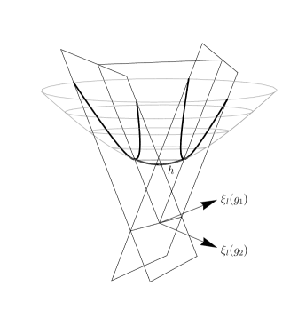
Figure 2: The distance $h$ between two geodesics in the unit hyperboloid $H_{1}$ is the hyperbolic angle between the corresponding planes through the origin in Minkowski space.

This raises the interesting question of how the two cases differ at the level of hyperbolic geometry. It turns out that when the two closed geodesics on the Riemann surface are non-intersecting (Fig. 3a), we have

$$|B(\xi_{l}(g_{1}),\xi_{l}(g_{2}))|=\cosh h>1,$$ (29)

where $h$ is the (shortest) hyperbolic distance between the two. If they do intersect (Fig. 3b), we have

$$B(\xi_{l}(g_{1}),\xi_{l}(g_{2}))=\cos\theta<1,$$ (30)

where $\theta$ is the angle between the geodesics at the intersection point. A simple way to see this is by considering the hyperboloid model $H_{1}$ (as described in C). The two geodesics define two planes through the origin in Minkowski space with normals equal to $\xi_{l}(g_{1})$ and $\xi_{l}(g_{2})$ (Fig. 2), and intersection spanned by the outer product $[\xi_{l}(g_{1}),\xi_{l}(g_{2})]$. The intersection will obviously only intersect $H_{1}$ if the two geodesics intersect on $H_{1}$, therefore $[\xi_{l}(g_{1}),\xi_{l}(g_{2})]$ is timelike if and only if the two geodesics intersect. Now there is a unique element $g\in PSL(2,\mathbb{R})$ for which $\mathrm{Ad}(g)$ maps $\xi_{l}(g_{1})$ to $\xi_{l}(g_{2})$ and leaves $[\xi_{l}(g_{1}),\xi_{l}(g_{2})]$ invariant.

If the commutator $[\xi_{l}(g_{1}),\xi_{l}(g_{2})]$ is spacelike, the group element $g$ is hyperbolic and $\xi_{l}(g)$ is proportional to $[\xi_{l}(g_{1}),\xi_{l}(g_{2})]$. From (22) we deduce that the scalar product of the two vectors is given by $B(\xi_{l}(g_{1}),\xi_{l}(g_{2}))=\cosh l(g)$. The invariant geodesic in $H_{1}$ corresponding to $g$ is the intersection of the plane spanned by $\xi_{l}(g_{1})$ and $\xi_{l}(g_{2})$ with $H_{1}$. It therefore coincides with the perpendicularly connecting geodesic, and the searched-for distance $h$ is just $l(g)$. On the other hand, if $[\xi_{l}(g_{1}),\xi_{l}(g_{2})]$ is timelike, the angle $\theta$ between the geodesics in $H_{1}$ is just the angle between the two planes, which satisfies $B(\xi_{l}(g_{1}),\xi_{l}(g_{2}))=\cos\theta$.

In order to calculate the variation of $B(\xi_{l}(g_{1}),\xi_{l}(g_{2}))$ (that is, of $h$ and $\theta$) to arrive at the Dirac length observable, we first need an identity for the derivative of $\xi_{l}(g)$, namely,

$$\left.\frac{\rmd}{\rmd t}\right|_{t=0}\xi_{l}(\exp(tX)g)=[Y,\xi_{l}(g)],$$ (31)

where $Y$ is a point on the invariant geodesic. To prove this, note that $\xi_{l}(\exp(t\xi_{l}(g))g)=\xi_{l}(g)$ for all $t$, which means that we can replace $X$ by $(\mathrm{Ad}(g)-1)Y$ according to (20),

$$\left.\frac{\rmd}{\rmd t}\right|_{t=0}\xi_{l}(\exp(tX)g) = \left.\frac{\rmd}{\rmd t}\right|_{t=0}\xi_{l}(\exp(t(\mathrm{Ad}(g)-1)Y)g)$$ (32)

$$= \left.\frac{\rmd}{\rmd t}\right|_{t=0}\xi_{l}(\exp(tY)g\exp(-tY))$$

$$= \left.\frac{\rmd}{\rmd t}\right|_{t=0}\mathrm{Ad}(\exp(tY))\xi_{l}(g)$$

$$= \left.\frac{\rmd}{\rmd t}\right|_{t=0}\exp(t\ \mathrm{ad}(Y))\xi_{l}(g)$$

$$= \mathrm{ad}(Y)\xi_{l}(g)=[Y,\xi_{l}(g)].$$

Using this result, we find for the variation of $B(\xi_{l}(g_{1}),\xi_{l}(g_{2}))$

$$\left.\frac{\rmd}{\rmd t}\right|_{t=0}B(\xi_{l}(\exp(tX_{1})g_{1}),\xi_{l}(\exp(tX_{2})g_{2}))$$

$$=B\left(\left.\frac{\rmd}{\rmd t}\right|_{t=0}\xi_{l}(\exp(tX_{1})g_{1}),\xi_{l}(g_{2})\right)$$

$$\quad+B\left(\xi_{l}(g_{1}),\left.\frac{\rmd}{\rmd t}\right|_{t=0}\xi_{l}(\exp(tX_{2})g_{2})\right)$$

$$=B([Y_{1},\xi_{l}(g_{1})],\xi_{l}(g_{2}))+B(\xi_{l}(g_{1}),[Y_{2},\xi_{l}(g_{2})])$$

$$=B(Y_{1}-Y_{2},[\xi_{l}(g_{1}),\xi_{l}(g_{2})]),$$ (33)

so that finally

$$\rmd h=\frac{\rmd\cosh h}{\sqrt{\cosh^{2}h-1}}=\frac{B(Y_{1}-Y_{2},[\xi_{l}(g_{1}),\xi_{l}(g_{2})])}{\sqrt{B(\xi_{l}(g_{1}),\xi_{l}(g_{2}))^{2}-1}},$$ (34)

and similarly for $\theta$. We conclude that

$$D_{\alpha_{1}\alpha_{2}}=\left\{\begin{array}[]{cl}\rmd\theta_{\alpha_{1}\alpha_{2}}&\alpha_{1},\alpha_{2}\;\mathrm{intersect\ on\ Riemann\ surface}\\ \rmd h_{\alpha_{1}\alpha_{2}}&\mathrm{otherwise}\end{array}\right.,$$ (35)

which is illustrated in Fig. 3.

(a)

(b)

Figure 3: Distance $D_{\alpha_{1}\alpha_{2}}$ between (a) spacelike and (b) timelike separated closed geodesics in Minkowski space and their relation to hyperbolic geometry.

From relations (29) and (30) it is now straightforward to give a geometric interpretation of the functions $\theta_{\alpha_{1}\alpha_{2}}$ and $h_{\alpha_{1}\alpha_{2}}$ on $\mathcal{P}$: $h$ is the hyperbolic angle (or boost parameter) between $\gamma_{1}$ and $\gamma_{2}$ measured along the connecting geodesic $c$, and $\theta$ is the angle between $\gamma_{1}$ and $\gamma_{2}$ along $c$. With regard to our quest for expressing geometric quantities in Minkowski space in terms of “Teichmüller data”, we can already see the general picture emerging: spacelike geodesics in Minkowski space are related to geodesics on the Riemann surface, and distances along them in Minkowski space correspond to variations of hyperbolic distances. By contrast, timelike geodesics relate to points in the Riemann surface, and timelike distances correspond to variations of angles at those points.

4 Quantization

In section 2.2 we identified the phase space $\mathcal{P}$ of 2+1 dimensional gravity with the cotangent bundle $T^{*}\mathcal{T}$ to Teichmüller space together with its canonical symplectic structure. Geometric quantization of this phase space is straightforward. As Hilbert space we take $\mathcal{H}=L^{2}(\mathcal{T},\omega_{WP}^{3g-3})$, the space of square-integrable wave functions on Teichmüller space with volume form defined by the Weil-Petersson symplectic structure $\omega_{WP}$. A function $f$ on Teichmüller space becomes a multiplication operator

$$\hat{f}\phi=f\cdot\phi,$$ (36)

and its variation $F$ a derivative operator according to

$$\hat{F}\phi=\rmi\hbar\{f,\phi\}_{WP}.$$ (37)

One easily checks that this yields an operator representation of the Poisson algebra (2.2) of phase space functions at most linear in the translational part of the holonomies. By the Stone-von Neumann theorem the quantization of the latter algebra is unique up to unitary equivalence, because our phase space can be brought globally to the canonical form $T^{*}\mathbb{R}^{6g-6}$.

The procedure for finding the spectrum of an operator $\hat{F}$ corresponding to the variation of a function $f$ on Teichmüller space $\mathcal{T}$ is relatively straightforward. The Hamiltonian vector field $H_{f}=\tilde{\omega}_{WP}^{-1}(\rmd f)$ generates the Hamiltonian flow of $f$ on $\mathcal{T}$. If we take a wave function $\phi$ with support on a single orbit $\mathcal{O}$ of the flow, it will be an eigenstate of $\hat{F}$ with eigenvalue $F$ if it describes a wave in the flow parameter $t$, that is,

$$\phi|_{\mathcal{O}}(t)\propto\exp(-\frac{\rmi}{\hbar}Ft).$$ (38)

Whether the spectrum of $\hat{F}$ (restricted to the orbit $\mathcal{O}$) is continuous or discrete depends on the domain of $t$. Whenever the flow is well-defined and injective for $t\in\mathbb{R}$, $F$ can take any value in $\mathbb{R}$. However, if $t$ is restricted to take values in a bounded interval, say, $t\in]0,r[$, we can only have a discrete set of eigenstates with eigenvalues $F$ which are separated by a distance $2\pi\hbar/r$. The precise eigenvalues depend on the chosen self-adjoint extension of $\hat{F}$ or, equivalently, on the chosen boundary conditions for $\phi$. To get the full spectrum of $F$ we must combine all spectra of the individual orbits, which need not coincide.

4.1 Spectra of length observables

Figure 4: The Hamiltonian vector field $H_{l_{\alpha}}$ generates a twist along $\alpha$.

Recall that the length of a closed geodesic is given by the variation $L_{\alpha}=\rmd l_{\alpha}$ of the hyperbolic length $l_{\alpha}$. A convenient global coordinate system for Teichmüller space is given by the Fenchel-Nielsen coordinates $(l_{i},\tau_{i})$, $i=1,\dots,3g-3$ (see C), corresponding to a pair-of-pants decomposition which has $\alpha$ as one of the cuts. In these coordinates the Weil-Petersson symplectic form is given by (86),

$$\omega_{WP}=\sum_{i}\rmd l_{i}\wedge\rmd\tau_{i},$$ (39)

where the $\tau_{i}$ are the twist parameters. The Hamiltonian flow of $l_{\alpha}$ is simply the twist flow along $\alpha$ (Fig. 4). Since the twist parameters as coordinates on Teichmüller space have domain equal to $\mathbb{R}$, we conclude that the spectrum of $\hat{L}_{\alpha}$ is the entire real line $\mathbb{R}$.

(a)

(b)

Figure 5: (a) Angle between two geodesics on the one-holed torus. (b) Cutting the torus open, one obtains an octagon, which can be put inside the Poincaré disc.

Next, we will investigate the operator

$$\hat{D}_{\alpha_{1}\alpha_{2}}=\rmi\hbar\{\theta,\cdot\}_{WP}$$ (40)

corresponding to a timelike distance between two geodesics. To start with, consider the geometric situation as depicted in Fig. 5, namely, a Riemann surface of genus 1 with a hole of geodesic boundary length $l_{0}$. Fixing $l_{0}$ means that its hyperbolic geometry is described by a two-dimensional Teichmüller space $\mathcal{T}$. Once we have found the spectrum of $\hat{D}_{\alpha_{1}\alpha_{2}}$, we will argue that the result holds for any spatial topology and for any two simple closed geodesics $\alpha_{1}$ and $\alpha_{2}$ with a single intersection.

One way of parametrizing $\mathcal{T}$ (up to a sign) is through the lengths $l_{1}$ and $l_{2}$ of $\gamma_{1}$ and $\gamma_{2}$ as indicated in Fig. 5. Cutting the surface along $\gamma_{1}$ and along two shortest geodesics connecting the hole’s boundary to either side of $\gamma_{1}$, we obtain an eight-sided polygon which we can draw at the centre of the Poincaré disc as in Fig. 5. Using the symmetries of the situation and applying the trigonometric identities from C we find that

$$\sinh\frac{l_{1}}{2}\sinh\frac{l_{2}}{2}\geq\cosh\frac{l_{0}}{4}$$ (41)

and

$$\sin\theta=\frac{\cosh\frac{l_{0}}{4}}{\sinh\frac{l_{1}}{2}\sinh\frac{l_{2}}{2}}.$$ (42)

In view of the explicit form (40) of the operator $\hat{D}$, we are particularly interested in the range of the variable conjugate to $\theta$, thus in finding a function $\rho$ on Teichmüller space satisfying

$$\{\theta,\rho\}_{WP}=1.$$ (43)

We will for the moment restrict our attention to only half of Teichmüller space, corresponding to $0<\theta<\frac{\pi}{2}$, for which we can use $l_{1}$ and $l_{2}$ as coordinates (with domain given by (41)). We can find an explicit solution for $\rho(l_{1},l_{2})$ by solving a partial differential equation which we obtain from (42) using Wolpert’s formula (87),

$$1=\{\theta,\rho\}_{WP} = \cos\theta\left(\frac{\partial\theta}{\partial l_{1}}\frac{\partial\rho}{\partial l_{2}}-\frac{\partial\theta}{\partial l_{2}}\frac{\partial\rho}{\partial l_{1}}\right)$$ (44)

$$= \frac{\partial(\sin\theta)}{\partial l_{1}}\frac{\partial\rho}{\partial l_{2}}-\frac{\partial(\sin\theta)}{\partial l_{2}}\frac{\partial\rho}{\partial l_{1}}$$

$$= \frac{\sin\theta}{2}\left(\coth\frac{l_{2}}{2}\frac{\partial\rho}{\partial l_{1}}-\coth\frac{l_{1}}{2}\frac{\partial\rho}{\partial l_{2}}\right).$$

This equation can be solved using standard techniques for first-order partial differential equations. The solution will be unique up to addition of a function of $\theta$, which obviously will Poisson-commute with $\theta$. To determine $\rho$ uniquely (up to a constant) we require it to be antisymmetric in $l_{1}$ and $l_{2}$. An uninspiring calculation then leads to

$$\rho=\frac{2}{\sin\theta}\mbox{sc}^{-1}\left(\frac{1}{2}\left(\frac{\cosh\frac{l_{1}}{2}}{\cosh\frac{l_{2}}{2}}-\frac{\cosh\frac{l_{2}}{2}}{\cosh\frac{l_{1}}{2}}\right)\middle|1-\frac{\sin^{2}\theta}{\cosh^{2}\frac{l_{0}}{4}}\right),$$ (45)

where $\mbox{sc}^{-1}$ is the inverse Jacobi elliptic function [34].

(a)

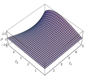
(b)

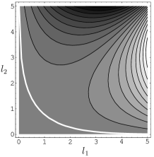
Figure 6: (a) Three-dimensional plot and (b) contour plot of $\rho$ as function of $l_{1}$ and $l_{2}$ (with $l_{0}=1$). The white line in (b) corresponds to $\sinh\frac{l_{1}}{2}\sinh\frac{l_{2}}{2}=\cosh\frac{l_{0}}{4}$. Note the antisymmetry with respect to exchange of $l_{1}$ and $l_{2}$.

For illustration, we show some Mathematica plots of $\rho$ as function of $l_{1}$ and $l_{2}$ for small $l_{i}$ in Fig. 6. It is not difficult to verify that

$$\quad\quad\left\{(l_{1},l_{2})\in\mathbb{R}_{>0}^{2}\middle|\sinh\frac{l_{1}}{2}\sinh\frac{l_{2}}{2}>\cosh\frac{l_{0}}{4}\right\}\to\left]0,\frac{\pi}{2}\right[\,\times\,\mathbb{R}:(l_{1},l_{2})\to(\theta,\rho)$$ (46)

is smooth and injective. By allowing $\theta$ to take values in $]0,\pi[$, we obtain global coordinates on Teichmüller space.

To find the domain of $\rho$ we note that $x\to\mbox{sc}^{-1}(x|m)$ is a bounded, strictly increasing function for fixed $m\in]-1,1[$. The asymptotic values are $\pm K(m)$ at $x\to\pm\infty$, where $K(m)$ is the complete elliptic integral of the first kind [34]. Hence, for fixed $\theta$ we have $-\frac{1}{2}\Delta\rho_{l_{0}}(\theta)<\rho<\frac{1}{2}\Delta\rho_{l_{0}}(\theta)$, where we have defined

$$\Delta\rho_{l_{0}}(\theta)=\frac{4}{\sin\theta}\ K\left(1-\frac{\sin^{2}\theta}{\cosh^{2}\frac{l_{0}}{4}}\right).$$ (47)

The function $\Delta\rho_{l_{0}}(\theta)$ has a minimum at $\theta=\pi/2$, where it assumes the value

$$\Delta\rho_{l_{0}}\left(\frac{\pi}{2}\right)=4\ K\left(\tanh^{2}\frac{l_{0}}{4}\right).$$ (48)

Computing the minimum as a function of $l_{0}$ (Fig. 7), one observes that it starts out at the value $2\pi$ at $l_{0}=0$ and for increasing $l_{0}$ converges rapidly to $l_{0}+c$ for a constant $c\approx 2.77$.

We conclude that the separation of the eigenvalues of $\hat{D}_{\alpha_{1}\alpha_{2}}$ depends on both $\theta$ and $l_{0}$ and is given by

$$D_{\alpha_{1}\alpha_{2}}\in\frac{2\pi}{\Delta\rho_{l_{0}}(\theta)}\hbar\,\mathbb{Z},$$ (49)

up to a constant which may depend on $\theta$ and $l_{0}$. For $\theta$ near $\pi/2$ and $l_{0}$ small the separation is approximately equal to the Planck length $\hbar$. However, the discretization disappears when $\theta\to 0,\pi$ or $l_{0}\to\infty$.

(a)

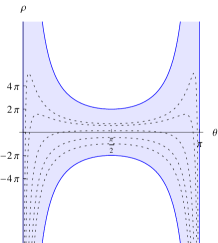
(b)

Figure 7: (a) The domain of $\rho$ and $\theta$ (shaded area). The dotted curves correspond to constant $l_{1}$. (b) The value of the minimum of $\Delta\rho$, as a function of $l_{0}$.

In order to complete our derivation, we still need to show that “isolating a handle”, as we did above (c.f. Fig. 5), does not constitute any loss of generality. Let $\Sigma$ be a Riemann surface of any genus $g\geq 2$, and $\alpha_{1}$ and $\alpha_{2}$ two simple closed geodesics on $\Sigma$ with precisely one intersection (an example with $g=2$ is depicted in Fig. 8). The unique closed geodesic $\alpha_{0}$ in the homotopy class $[\alpha_{1}][\alpha_{2}][\alpha_{1}]^{-1}[\alpha_{2}]^{-1}$ is necessarily disjoint from $\alpha_{1}$ and $\alpha_{2}$. A pair-of-pants decomposition containing $\alpha_{0}$ and $\alpha_{1}$ as cuts will then contain one pair of pants which has the form of a one-holed torus, as in our previous calculation, the only difference being that $l_{0}$ is no longer an external parameter, but a function on Teichmüller space. The symplectic structure is given by

$$\omega_{WP}=\rmd l_{0}\wedge\rmd\tau_{0}+\rmd l_{1}\wedge\rmd\tau_{1}+\sum_{i=2}^{3g-2}\rmd l_{i}\wedge\rmd\tau_{i},$$ (50)

with $l_{1}=l(\alpha_{1})$, which can be rewritten as

$$\omega_{WP}=\rmd l_{0}\wedge\rmd\tilde{\tau}_{0}+\rmd\theta\wedge\rmd\rho+\sum_{i=2}^{3g-2}\rmd l_{i}\wedge\rmd\tau_{i},$$ (51)

where $\tilde{\tau}_{0}=\tau_{0}+\Delta\tau_{0}(l_{0},l_{1},\tau_{1})$ and $\Delta\tau_{0}$ is a function satisfying

$$\frac{\partial\Delta\tau_{0}}{\partial\tau_{1}}=\frac{\partial\theta}{\partial\tau_{1}}\frac{\partial\rho}{\partial l_{0}}-\frac{\partial\theta}{\partial l_{0}}\frac{\partial\rho}{\partial\tau_{1}},\quad\frac{\partial\Delta\tau_{0}}{\partial l_{1}}=\frac{\partial\theta}{\partial l_{1}}\frac{\partial\rho}{\partial l_{0}}-\frac{\partial\theta}{\partial l_{0}}\frac{\partial\rho}{\partial l_{1}}.$$ (52)

One can check that these differential equations are consistent, that is, $\partial^{2}\Delta\tau_{0}/\partial l_{1}\partial\tau_{1}=\partial^{2}\Delta\tau_{0}/\partial\tau_{1}\partial l_{1}$, and therefore can always be solved. We conclude that $\theta,\rho,l_{0},\tilde{\tau}_{0},l_{i},\tau_{i}$ form a new coordinate system for Teichmüller space in which $\omega_{WP}$ is given by (51). This means that the spectrum of $\hat{D}_{\alpha_{1}\alpha_{2}}$ we found for the one-holed torus is valid in this case too.

Figure 8: A Riemann surface with two simple closed geodesics $\alpha_{1}$ and $\alpha_{2}$ intersecting with angle $\theta$.

A similar argument can be made in the case that the geodesics $\alpha_{1}$ and $\alpha_{2}$ do not intersect on $\Sigma$. Recall that the corresponding spacelike distance $D_{\alpha_{1}\alpha_{2}}$ was the variation of the hyperbolic length $h_{\alpha_{1}\alpha_{2}}$ of the geodesic connecting them. Also in this case one can always find a pair-of-pants decomposition having a particular pair of pants with $\alpha_{1}$, $\alpha_{2}$ and a third simple closed geodesic $\alpha_{0}$ as boundary components, and which contains the connecting geodesic. Since the geometry of a pair of pants is fully determined by the lengths of its boundary components $l_{1}$, $l_{2}$ and $l_{0}$, the length $h_{\alpha_{1}\alpha_{2}}$ as a function of the Fenchel-Nielsen coordinates also depends on $l_{1}$, $l_{2}$ and $l_{0}$ only, and we can write

$$\hat{D}_{\alpha_{1}\alpha_{2}}=i\hbar\left(\frac{\partial h}{\partial l_{1}}\frac{\partial}{\partial\tau_{1}}+\frac{\partial h}{\partial l_{2}}\frac{\partial}{\partial\tau_{2}}+\frac{\partial h}{\partial l_{0}}\frac{\partial}{\partial\tau_{0}}\right).$$ (53)

Just as in the case of $\hat{L}_{\alpha}$, the Hamiltonian flow is a linear flow in the twist parameters and therefore the spectrum of $\hat{D}_{\alpha_{1}\alpha_{2}}$, for spacelike distances ${D}_{\alpha_{1}\alpha_{2}}$, is again continuous.

5 Discussion and conclusion

In this paper, we have identified space- and timelike length variables in 2+1 dimensional gravity with vanishing cosmological constant. They are given in terms of functions on the reduced phase space of the theory, obtained in a Chern-Simons formulation of the three-dimensional Poincaré group. Being linear in momenta, the quantization of these Dirac observables is essentially unique. A study of their eigenvalues in the quantum theory revealed continuous spectra spanning the entire real line for both space- and timelike distance operators. As far as we are aware, this constitutes the first rigorous derivation of quantum spectra of Dirac length observables in Lorentzian three-dimensional gravity for genus $g\geq 2$.

Although our results do not confirm previous investigations in [35, 11], which found evidence for a discrete spectrum for timelike distances, we did come across some discrete aspects in our spectral analysis. Although none of the length observables we considered were canonically conjugate to an angle, the timelike distance $D_{\alpha_{1}\alpha_{2}}$ was found to be conjugate to a function with a finite domain. However, the size of this domain is not bounded as a function on Teichmüller space (the habitat of the wave functions), which implies that there is no “spectral gap” for timelike distances.

The discrepancy with previous results may have to do with the fact that neither of them was based on a complete and consistent quantization of the theory on the reduced, physical phase space. The underlying formulations are sufficiently different from ours to make a direct comparison difficult. Subtleties with regard to the implementation of the Hamiltonian constraint [9, 4, 5] may well play a role. They can be seen as part of a larger issue, present in all but the simplest systems with gauge symmetry, namely, to what extent quantization and the imposition of constraints commute [37, 38]. Not even for the case of gravity on a spatial torus ($g=1$), whose quantization has received a lot of attention in the physics literature [10] has the question of the equivalence or otherwise of different quantizations been settled completely. Part of the problem is the scarcity of “observables” which one would like to use to compare physical results.

The generic presence of quantization ambiguities highlights the fact that the issue of “fundamental discreteness” can be interpreted in more than one way, depending on which quantization and operators one applies it to, and therefore may not have a unique answer. In the present work, we have focused on the well-defined notion of investigating the spectra of Dirac observables measuring lengths, obtained in a “time-less” phase space reduction of three-dimensional quantum gravity. One could argue that this setting is distinguished, because of the absence of any choice of time-slicing and the simplicity of the ensuing (Schrödinger) quantization.

The results we have been able to derive come with some qualifications. Firstly, as already mentioned earlier, the lengths $L_{\alpha}$ and $D_{\alpha_{1}\alpha_{2}}$ are not interpretable directly as lengths of curves (or of distances between such curves) inside the spacetime manifold itself. This happens because there are no closed geodesics in a nondegenerate solution in the class of geometries we have been considering (recall that each solution is obtained by making identifications on a convex open subset of 3d Minkowski space). Nevertheless, they constitute a complete set of length variables “associated with a solution”, in terms of which any other observable can be expressed. By the same token, we do not claim that our length variables are directly measurable.

There are related constructions which may yield length observables with a more immediate physical interpretation. For example, we could consider the length of a path in a particular homotopy class in the limit as it approaches the initial singularity, or the lengths of closed geodesics in a surface of constant cosmological time [26]. In either case it is difficult to characterize the corresponding functions on Teichmüller space explicitly. To quantize them one should reformulate the phase space entirely in terms of so-called measured laminations. This may be feasible, in the sense that these structures are well studied and a lot is known about the relevant symplectic structure [39, 40, 25, 33].

Another possibility of constructing physical observables is by enlarging the phase space slightly. It is straightforward to include point particles into the model, although there are some subtleties which prevent the naïve use of a quotient construction to obtain the spacetime. The world lines of massive particles define timelike geodesics and one could consider measuring minimal distances between them. An alternative method proposed recently by Meusburger [33] is to define diffeomorphism-invariant observables corresponding to geodesics (in this case light-like), but parametrized by the eigentime along the worldline of an observer. They are an example of Rovelli’s evolving constants of motion [41, 19].

Note that in our investigation we have only considered length spectra associated with a subset of curves, namely, particular geodesics (i.e. straight lines) in Minkowski space. Our construction does not allow for an easy generalization to arbitrary curves. This, and the peculiar behaviour we found when analyzing the spectrum of the timelike distance between two spacelike geodesics in the previous section, namely, that the discretization unit of this distance depends on the relative angle between the geodesics, are an expression of the fact that the only dynamical degrees of freedom of the theory are of a global nature, and are captured in a coupled and nonlocal way by various length variables. This is not a feature one would expect to be present in four dimensions, where the metric does possess local degrees of freedom.

The Lorentzian nature of the spacetime was crucial for deriving the results presented here. If we replaced the Poincaré group $ISO(2,1)$ with the Euclidean group $ISO(3)$, we would obtain a theory closely related to the Euclidean lattice gravity model of Ponzano and Regge [42], whose phase space can be identified with the tangent bundle to (a suitable subspace of) the space of flat $SU(2)$-connections on $\Sigma$. One can repeat the constructions of Sec. 3 in terms of invariant geodesics to obtain the analogues of the functions $L_{\alpha}$ and $D_{\alpha_{1}\alpha_{2}}$. The quantization is completely analogous, with $\hat{L}_{\alpha}$ generating a so-called generalized twist flow [30] on the $SU(2)$-equivalent of Teichmüller space. However, it turns out that this twist flow is periodic with fixed period [43], which implies that the spectrum of $\hat{L}_{\alpha}$ will be discretized in units of a fixed minimal length of the order of the Planck length. This is in complete agreement with results obtained in the loop representation [44].

Finally, one may wonder whether any of the techniques we have used can be extended to $3+1$ dimensions. An obvious starting point would be a generalization to topological field theories with a different gauge group. One such theory, perhaps closest to general relativity in $3+1$ dimensions, is BF theory [45] with gauge group $SO(3,1)$. Since $SO_{0}(3,1)$ is isomorphic to $PSL(2,\mathbb{C})$, the isometry group of three-dimensional hyperbolic space, one should be able to relate some length observables in a flat $3+1$ dimensional spacetime to functions in three-dimensional hyperbolic geometry. Further research is needed to determine whether this is feasible. Another connection worthwhile pursuing may be the generalization to $3+1$ dimensions of $2+1$ gravity with point particles formulated recently by ’t Hooft [46].

Acknowledgements. RL acknowledges support by ENRAGE (European Network on Random Geometry), a Marie Curie Research Training Network in the European Community’s Sixth Framework Programme, network contract MRTN-CT-2004-005616, and by the Netherlands Organisation for Scientific Research (NWO) under their VICI program.

Appendix A The gauge group

We denote the future-preserving Lorentz group in 2+1 dimensions by $SO_{0}(2,1)$, which is precisely the identity component of $SO(2,1)$. A basis for its Lie algebra $\mathfrak{so}(2,1)$ is given by

$$\quad\quad\begin{array}[]{ccc}J_{0}^{\mathfrak{so}}=\left(\begin{array}[]{ccc}0&0&0\\ 0&0&1\\ 0&-1&0\end{array}\right)&J_{1}^{\mathfrak{so}}=\left(\begin{array}[]{ccc}0&0&-1\\ 0&0&0\\ -1&0&0\end{array}\right)&J_{2}^{\mathfrak{so}}=\left(\begin{array}[]{ccc}0&-1&0\\ -1&0&0\\ 0&0&0\end{array}\right).\end{array}$$ (54)

satisfying the commutation relations $[J_{a},J_{b}]={\epsilon_{ab}}^{c}J_{c}$, where the totally antisymmetric $\epsilon$-tensor is defined by $\epsilon_{012}=-\epsilon^{012}=1$, and indices are raised and lowered with the metric $\eta_{ab}={\rm diag}(-1,1,1)$. The generators $J_{a}^{\mathfrak{so}}$ form an orthonormal basis with respect to the indefinite bilinear form

$$B^{\mathfrak{so}}(X,Y)=\frac{1}{2}\Tr(XY),\;\;\;\;\;B^{\mathfrak{so}}(J_{a}^{\mathfrak{so}},J_{b}^{\mathfrak{so}})=\eta_{ab}.$$ (55)

We will often use the isomorphism $SO_{0}(2,1)\cong PSL(2,\mathbb{R})=SL(2,\mathbb{R})/\{I,-I\}$. To make the isomorphism explicit we choose the specific basis

$$\begin{array}[]{ccc}J_{0}^{\mathfrak{sl}}=\frac{1}{2}\left(\begin{array}[]{cc}0&-1\\ 1&0\end{array}\right)&J_{1}^{\mathfrak{sl}}=\frac{1}{2}\left(\begin{array}[]{cc}1&0\\ 0&-1\end{array}\right)&J_{2}^{\mathfrak{sl}}=\frac{1}{2}\left(\begin{array}[]{cc}0&1\\ 1&0\end{array}\right)\end{array}$$ (56)

for the Lie algebra $\mathfrak{sl}(2,\mathbb{R})$. The generators satisfy identical commutation relations and are orthonormal with respect to the bilinear form

$$B^{\mathfrak{sl}}(X,Y)=2\Tr(XY),\;\;\;\;\;B^{\mathfrak{sl}}(J_{a}^{\mathfrak{sl}},J_{b}^{\mathfrak{sl}})=\eta_{ab}.$$ (57)

In fact, $SO_{0}(2,1)$ emerges as the adjoint representation of $PSL(2,\mathbb{R})$ on $\mathfrak{sl}(2,\mathbb{R})$, when written in the basis (56).

The gauge group of 2+1 gravity is the 2+1 dimensional Poincaré group $ISO_{0}(2,1)$, which is most easily characterized as the semi-direct product of $SO_{0}(2,1)$ and the abelian group $\mathbb{R}^{3}$, where the action of $SO_{0}(2,1)$ on $\mathbb{R}^{3}$ is the fundamental one, namely,

$$(g_{1},X_{1})\cdot(g_{2},X_{2})=(g_{1}g_{2},X_{1}+g_{1}X_{2}).$$ (58)

In terms of the basis (54), we can identify $\mathfrak{so}(2,1)$ with $\mathbb{R}^{3}$, where the action of $SO_{0}(2,1)$ now becomes the adjoint action,

$$(g_{1},X_{1})\cdot(g_{2},X_{2})=(g_{1}g_{2},X_{1}+\mathrm{Ad}(g_{1})X_{2}).$$ (59)

In this way we identify $ISO_{0}(2,1)$ with $SO_{0}(2,1)\ltimes\mathfrak{so}(2,1)$, which is again isomorphic to $PSL(2,\mathbb{R})\ltimes\mathfrak{sl}(2,\mathbb{R})$.

Furthermore, for any Lie group $G$ its semi-direct product group $G\ltimes\mathfrak{g}$ is isomorphic to its tangent group $TG$, which is defined by taking as multiplication the tangent map to the multiplication map $G\times G\to G$. Explicitly, the isomorphism, which elsewhere we often use implicitly, identifies the elements of the Lie algebra $\mathfrak{g}$ with the right-invariant vector fields on $G$. – To summarize, we have the following chain of isomorphisms

$$ISO_{0}(2,1) \cong SO_{0}(2,1)\ltimes\mathfrak{so}(2,1)\cong PSL(2,\mathbb{R})\ltimes\mathfrak{sl}(2,\mathbb{R})$$ (60)

$$\cong T\,SO_{0}(2,1)\cong T\,PSL(2,\mathbb{R}).$$

Finally, a nondegenerate bilinear form on $\mathfrak{g}$ gives rise to a natural bilinear form on the Lie algebra of $TG$ by taking its derivative. For the case at hand, we obtain a natural nondegenerate bilinear form on $\mathfrak{iso}(2,1)\cong\mathfrak{so}(2,1)\times\mathfrak{so}(2,1)$ by defining

$$B\left((X_{1},Y_{1}),(X_{2},Y_{2})\right)=B^{\mathfrak{so}}(X_{1},Y_{2})+B^{\mathfrak{so}}(Y_{1},X_{2}).$$ (61)

Appendix B Some group theory

For a Lie group $G$ and its associated Lie algebra $\mathfrak{g}$, we denote the left and right multiplication maps by $l_{g},r_{g}:G\to G$. The conjugation map $C_{g}:x\to gxg^{-1}$ is an isomorphism of $G$ to itself and its tangent map at the origin $\mathrm{Ad}(g)=T_{e}C_{g}$ is the adjoint representation acting on $\mathfrak{g}$. Suppose $B$ is a nondegenerate invariant (pseudo-) metric on $G$, i.e. $B:\mathfrak{g}\times\mathfrak{g}\to\mathbb{R}$ is a nondegenerate bilinear form invariant under adjoint transformations. We denote by $\tilde{B}$ the associated map $\mathfrak{g}\to\mathfrak{g}^{*}$.

To a differentiable function $f:G\to\mathbb{R}$ we can associate a natural map $\hat{\xi}_{f}:G\to\mathfrak{g}^{*}$, which is the right translation of the derivative of $f$ to the Lie algebra,

$$\hat{\xi}_{f}(g)=(T_{e}r_{g})^{*}\rmd f(g).$$ (62)

Using the metric $B$, we can define the variation $\xi_{f}=\tilde{B}^{-1}\circ\hat{\xi}_{f}:G\to\mathfrak{g}$ of $f$ [30]. Equivalently,

$$B(\xi_{f}(g),X)=\left.\frac{\rmd}{\rmd t}\right|_{t=0}f(\exp(tX)g)$$ (63)

for $X\in\mathfrak{g}$. Here $\exp:\mathfrak{g}\to G$ is the standard exponential map for Lie groups.

From now on will we assume $f$ to be a class function, i.e. a function which is invariant under conjugation, $C_{g}^{*}f=f$ for all $g\in G$. Using the well-known identity $C_{h}\circ\exp=\exp\circ\mathrm{Ad}(h)$, we find that

$$\xi_{f}(hgh^{-1})=\mathrm{Ad}(h)\xi_{f}(g).$$ (64)

Putting $h=g$ we see that $\xi_{f}(g)$ is invariant under $\mathrm{Ad}(g)$,

$$\mathrm{Ad}(g)\xi_{f}(g)=\xi_{f}(g).$$ (65)

Consider now the specific case $G=PSL(2,\mathbb{R})$ with the metric as in (57). For hyperbolic elements $g\in G_{hyp}=\{g|\Tr(g)>2\}\subset G$, we define the hyperbolic length $l(g)$ of $g$ by

$$\Tr(g)=2\cosh(l(g)/2).$$ (66)

Due to the cyclicity of the trace, $l$ is a class function, whose variation we can compute in a straightforward manner. Applying relation (63), we find for diagonal elements $g$ that $\xi_{l}(g)=\mathrm{diag}(1/2,-1/2)$. For general elements $g\in G_{hyp}$ which are diagonalized by $h\in G$, we have $\xi_{l}(g)=\mathrm{Ad}(h)\mathrm{diag}(1/2,-1/2)$. In particular, $\xi_{l}(g)$ is spacelike, of unit norm and the group element can be written as [30]

$$g=\exp(l(g)\xi_{l}(g)).$$ (67)

If desired, these two conditions can be taken as the definition of $l(g)$ and $\xi_{l}(g)$, because the exponential map is a bijection from $\{X\in\mathfrak{sl}(2,\mathbb{R})|B(X,X)>0\}$ to $G_{hyp}$. One can write the exponential in (67) explicitly as

$$g=\cosh\frac{l(g)}{2}\ 1+\left(2\sinh\frac{l(g)}{2}\right)\xi_{l}(g)$$ (68)

and

$$\quad\quad\quad\mathrm{Ad}(g)=\cosh l(g)\ 1+(1-\cosh l(g))\xi_{l}(g)B(\xi_{l}(g),\cdot)+\sinh l(g)[\xi_{l}(g),\cdot].$$ (69)

For elliptic elements we have a similar construction. We define $\theta(g)\in[0,2\pi[$ by $\Tr(g)=2\cos(\theta/2)$. In that case, $\xi_{\theta}(g)$ is timelike, of unit norm and the group element can be written as

$$g=\exp(\theta(g)\xi_{\theta}(g)).$$ (70)

Appendix C Hyperbolic geometry

In this appendix we will briefly review some notions of hyperbolic geometry, which are used in the main text (see, for example, [47] for details and proofs). For our purposes, “hyperbolic geometry” will mean the study of Riemann surfaces and geometric constructions on them. A Riemann surface is a two-dimensional real manifold with a complex structure. In this article we consider only compact oriented Riemann surfaces, which are topologically classified by their genus $g$. We will be concerned only with the case $g\geq 2$.

Let $\Sigma$ be a surface of genus $g\geq 2$. Its fundamental group is generated by a set of $2g$ homotopy classes of closed curves $\{a_{i},b_{i}\}_{i=1,\ldots,g}$ satisfying the relation

$$\prod_{i=1}^{g}a_{i}b_{i}a_{i}^{-1}b_{i}^{-1}=1.$$ (71)

The space of inequivalent complex structures on $\Sigma$ is called the moduli space $\mathcal{M}_{g}$ and depends only on the genus $g$. In the following we will consider a slightly larger space, the Teichmüller space $\mathcal{T}_{g}$, which is the universal covering of $\mathcal{M}_{g}$. One can define Teichmüller space as the space of equivalence classes of marked Riemann surfaces. “Marked” implies that we pick a complex structure and a distinguished set of generators for the fundamental group. Equivalently, we identify two complex structures on $\Sigma$ if they are related by a biholomorphism homotopic to the identity map. The moduli space can be obtained from Teichmüller space by taking the quotient with respect to the mapping class group,

$$\mathcal{M}_{g}=\mathcal{T}_{g}/\mathcal{MCG}.$$ (72)

It is well known that elements of the space of complex structures on $\Sigma$ are in one-to-one correspondence with conformally inequivalent metrics on $\Sigma$. Moreover, for the case $g\geq 2$, every conformal equivalence class contains a unique hyperbolic metric, i.e. a metric with constant curvature $-1$. Consequently, we can identify Teichmüller space with the space of hyperbolic metrics on $\Sigma$ modulo diffeomorphisms connected to the identity.

Next, consider a surface $\Sigma$ with a specific complex structure. As a consequence of the well-known uniformization theorem, the universal cover of $\Sigma$ is the complex upper half-plane $\mathbb{H}$. Any element of the fundamental group of $\Sigma$ therefore corresponds to an automorphism of $\mathbb{H}$. The automorphism group of $\mathbb{H}$ is easily seen to be equal to $PSL(2,\mathbb{R})$, acting according to

$$\left(\begin{array}[]{cc}a&b\\ c&d\end{array}\right):z\to\frac{az+b}{cz+d}.$$ (73)

An element $g\in PSL(2,\mathbb{R})$ which is not equal to the identity is said to be hyperbolic if $|\Tr(g)|>2$, elliptic if $|\Tr(g)|<2$ and parabolic if $\Tr(g)=2$. Under the identification $PSL(2,\mathbb{R})\cong SO_{0}(2,1)$ these correspond to boosts, rotations and lightlike transformations respectively. On $\mathbb{H}$, they can be characterized as those transformations which leave fixed two, no and one points on the boundary respectively.

The set $\Gamma$ of automorphisms corresponding to the elements of the fundamental group is called a Fuchsian model of $\Sigma$. We can write $\Sigma$ as the quotient

$$\Sigma=\mathbb{H}/\Gamma.$$ (74)

Since $\Sigma$ is a smooth manifold, $\Gamma$ must act properly discontinuously on $\mathbb{H}$, which is equivalent to $\Gamma$ being a Fuchsian group, that is, a discrete subgroup of $PSL(2,\mathbb{R})$. Such a group necessarily consists only of hyperbolic elements (and the identity). It turns out that any representation of the fundamental group $\pi_{1}$ as a Fuchsian group in $PSL(2,\mathbb{R})$ arises as the Fuchsian model of a complex structure. We therefore can identify Teichmüller space as

$$\mathcal{T}_{g}=\mathrm{Hom}_{0}(\pi_{1}(\Sigma),PSL(2,\mathbb{R}))/PSL(2,\mathbb{R}),$$ (75)

where the subscript 0 means that we restrict to injective homomorphisms which have a Fuchsian group as image.

(a)

(b)

Figure 9: Some geodesics in (a) the complex upper-half plane $\mathbb{H}$ and (b) the Poincaré disc $\Delta$.

To establish the geometric properties of a Riemann surface it suffices to know the geometry of its universal covering $\mathbb{H}$. The hyperbolic metric on $\mathbb{H}$ corresponding to its complex structure is the Poincaré metric $\rmd s^{2}_{\mathbb{H}}=|\rmd z|^{2}/\mathrm{Im}^{2}z$. The geodesics with respect to this metric are half circles centered on the real axis (see Fig. 9). Sometimes it is convenient to use an equivalent model of the hyperbolic plane, the Poincaré disc $\Delta$ with the Poincaré metric

$$\rmd s^{2}_{\Delta}=\frac{4|\rmd z|^{2}}{(1-|z|^{2})^{2}}.$$ (76)

Now the geodesics are circle arcs perpendicular to the boundary (see Fig. 9).

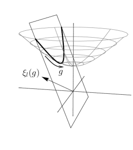
Figure 10: The hyperboloid model.

Yet another representation of the hyperbolic plane, which makes the relation to 2+1 dimensional spacetime most transparent, is the hyperboloid model. It is defined as the unit hyperboloid

$$H_{1}=\{X\in\mathbb{R}^{3}|X\cdot X=-1,X^{0}>0\}$$ (77)

in three-dimensional Minkowski space, as depicted in Fig. 10, with the induced metric. The geodesics are given by the intersections of $H_{1}$ with two-dimensional planes through the origin. An element $g\in PSL(2,\mathbb{R})\cong SO_{0}(2,1)$ acts on $H_{1}$ by Lorentz transformation (the adjoint representation $\mathrm{Ad}(g)$ of $g$, if we identify Minkowski space with $\mathfrak{sl}(2,\mathbb{R})$). If $g$ is hyperbolic, it corresponds to a boost in Minkowski space. Such a boost leaves a unique plane through the origin invariant and thus $g$ determines a unique invariant geodesic in $H_{1}$. Note that $\xi_{l}(g)$ is the normal to this plane, since it is invariant under $\mathrm{Ad}(g)$.

Trigonometry can be developed in the hyperbolic plane in analogy with the Euclidean case. We state here some trigonometric relations [48] for hyperbolic polygons, which are used in the main text. Referring to the notation of Fig. 11, they are

(a)

(b)

(c)

Figure 11: Examples of hyperbolic polygons. All unlabelled angles are right angles.

• Given any three numbers $a,b,c\in\mathbb{R}_{>0}$ there exists a unique convex right-angled hexagon with alternating sides of length $a$, $b$ and $c$. The lengths of the sides satisfy the relations

  $$\frac{\sinh a}{\sinh a^{\prime}}=\frac{\sinh b}{\sinh b^{\prime}}=\frac{\sinh c}{\sinh c^{\prime}},$$ (78)

  $$\cosh a^{\prime}=\frac{\cosh b\cosh c+\cosh a}{\sinh b\sinh c}.$$ (79)

  Analogous relations hold for $b^{\prime}$ and $c^{\prime}$.

• A pentagon with four right angles and a remaining angle $\alpha$ satisfies

  $$\frac{\sinh a}{\sin\alpha}=\frac{\cosh b}{\sinh b^{\prime}}=\frac{\cosh c}{\sinh c^{\prime}},$$ (80)

  $$\cosh a=\sinh b\sinh c-\cosh b\cosh c\cos\alpha.$$ (81)

• A triangle with arbitrary angles satisfies

  $$\frac{\sinh a}{\sin\alpha}=\frac{\sinh b}{\sin\beta}=\frac{\sinh c}{\sin\gamma},$$ (82)

  $$\cosh a=\cosh b\cosh c-\sinh b\sinh c\cos\alpha.$$ (83)

We saw above that a hyperbolic element $g\in PSL(2,\mathbb{R})$ leaves exactly two points on the boundary of the complex upper-half plane $\mathbb{H}$ fixed, which implies that there is a unique geodesic in $\mathbb{H}$ invariant under $g$. The geodesic is translated along itself by a hyperbolic distance $l(g)$, which is related to the trace of $g$ through eq. (66). If $g$ is an element of the Fuchsian model of $\Sigma$ corresponding to a homotopy class $\alpha$, this geodesic projects to the unique closed geodesic in $\alpha$ with length given by $l(g)$.

Closed geodesics on the Riemann surface are associated with a convenient set of coordinates on Teichmüller space, known as the Fenchel-Nielsen coordinates. Given a Riemann surface $\Sigma$ of genus $g\geq 2$, one can always find a set of $3g-3$ mutually disconnected simple (that is, non-selfintersecting) closed geodesics $\{\gamma_{i}\}$. Cutting the surface along these geodesics results in a decomposition of $\Sigma$ into $2g-2$ pairs of pants, each one a genus-0 Riemann surface with three geodesic boundary components. It is not hard to show (using the trigonometric identity (a) above) that the complex structure on a pair of pants is completely determined by the lengths of its boundary components. In order to fix the complex structure on $\Sigma$ we therefore need to fix the lengths $l_{i}$ of the geodesics $\gamma_{i}$ and the way we re-glue the pairs of pants. To quantify the latter we introduce the so-called twist parameters $\tau_{i}$, which measure the distance between particular distinguished points on $\gamma_{i}$. It turns out that both types of variables taken together,

$$(l_{i},\tau_{i})\in(\mathbb{R}_{>0}\times\mathbb{R})^{3g-3},$$ (84)

form a global set of coordinates on Teichmüller space. In particular, this implies that

$$\dim\mathcal{T}_{g}=6g-6.$$ (85)

The Weil-Petersson symplectic structure (see D) takes on a particularly simple form in terms of the Fenchel-Nielsen coordinates [47], namely,

$$\omega_{WP}=\sum_{i=1}^{3g-3}\rmd l_{i}\wedge\rmd\tau_{i}.$$ (86)

For two closed geodesics $\alpha$ and $\beta$, the Poisson bracket of their associated lengths variables is given by Wolpert’s formula,

$$\{l_{\alpha},l_{\beta}\}_{WP}=\sum_{p\in\alpha\sharp\beta}\cos\theta_{p},$$ (87)

where the sum runs over the intersection points $p$ and $\theta_{p}$ is the angle between $\alpha$ and $\beta$ at $p$. Note that we could have derived this formula by combining (30) with (89) (see also [30]).

Appendix D Generalized Weil-Petersson symplectic structure

For a compact oriented surface $\Sigma$ of genus $g>1$, we are interested in homomorphisms from its fundamental group $\pi_{1}$ to a Lie group $G$. More specifically, we want to consider the space $\mbox{Hom}(\pi_{1},G)/G$, where $G$ acts on $\mbox{Hom}(\pi_{1},G)$ by overall conjugation. For a homomorphism $\phi:\pi_{1}\rightarrow G$, we will denote its equivalence class by $[\phi]\in\mbox{Hom}(\pi_{1},G)/G$.

If $G$ possesses a (pseudo-)metric, i.e. a nondegenerate bilinear form $B$ on its Lie algebra $\mathfrak{g}$, (a suitable open subset of) the space $\mbox{Hom}(\pi_{1},G)/G$ can be given a canonical symplectic structure $\omega_{G}$, known as the generalized Weil-Petersson symplectic structure. Without giving any details of the construction, which involves homology, we will simply state the main result of [49]. For a class function $f$ on $G$ (see B) and a closed curve $\alpha$ in $\Sigma$, define

$$f_{\alpha}:\mbox{Hom}(\pi_{1},G)/G\rightarrow\mathbb{R}:[\phi]\rightarrow f(\phi([\alpha])).$$ (88)

Given two such functions, $f$ and $f^{\prime}$, and two closed curves $\alpha$ and $\alpha^{\prime}$, the Poisson bracket of $f_{\alpha}$ and $f^{\prime}_{\alpha^{\prime}}$ turns out to be

$$\{f_{\alpha},f^{\prime}_{\alpha^{\prime}}\}_{G}([\phi])=\sum_{p\in\alpha\sharp\alpha^{\prime}}\varepsilon(p;\alpha,\alpha^{\prime})B(\xi_{f}(\phi(\alpha_{p})),\xi_{f^{\prime}}(\phi(\alpha^{\prime}_{p}))),$$ (89)

where $\alpha\sharp\alpha^{\prime}$ is the set of intersections in $\Sigma$. The discrete variable $\varepsilon(p;\alpha,\alpha^{\prime})=\pm 1$ depends on the orientation of the intersection, $\alpha_{p}$ is just the curve $\alpha$ but with base point specified to be $p$, and $\xi_{f}:G\to\mathfrak{g}$ is the variation of $f$ as defined in B.

The above can also be applied to the tangent group $TG$, which was introduced in A, together with the metric

$$B_{TG}((X_{1},Y_{1}),(X_{2},Y_{2}))=B(X_{1},Y_{2})+B(Y_{1},X_{2}),$$ (90)

which is essentially the derivative of $B$. We will now show that the generalized Weil-Petersson symplectic form $\omega_{TG}$ for the group $TG$ is the tangent symplectic form corresponding to $\omega_{G}$. Instead of $TG$ we will use the semi-direct product $G\ltimes\mathfrak{g}$, which is isomorphic to $TG$ by right translation (see A).

Let $f:G\to\mathbb{R}$ be a class function on $G$ (see B). We associate to $f$ two class functions on $G\ltimes\mathfrak{g}$, its trivial extension $\hat{f}=f\circ\pi_{G}$ and its variation $F:(g,X)\to B(\xi_{f}(g),X)$. To compute the Poisson brackets (89) we will need the variations of both $\hat{f}$ and $F$. The variation of $\hat{f}$ is easily seen to be given by $\xi_{\hat{f}}(g,X)=(0,\xi_{f}(g))\in\mathfrak{g}\times\mathfrak{g}$. The variation of $F$ is a bit trickier. From definition (62) we have

$$\quad\quad B_{TG}(\xi_{F}(g,X),(Y,Z)) = \rmd F((g,X),T_{e}r_{(g,X)}(Y,Z))$$ (91)

$$= \left.\frac{\rmd}{\rmd s}\right|_{s=0}F\left(\exp(sY)g,X+sZ+s[Y,X])\right)$$

$$= \left.\frac{\rmd}{\rmd t}\right|_{t=0}\left.\frac{\rmd}{\rmd s}\right|_{s=0}f\left(\exp(tX+tsZ+ts[Y,X])\exp(sY)g\right)$$

$$= \left.\frac{\rmd}{\rmd t}\right|_{t=0}\left.\frac{\rmd}{\rmd s}\right|_{s=0}f\left(\exp(sY)\exp(tX+tsZ)g\right)$$

$$= B(\xi_{f}(g),Z)+\left.\frac{\rmd}{\rmd t}\right|_{t=0}B(\xi_{f}(\exp(tX)g),Y).$$

Hence

$$\xi_{F}(g,X)=\left(\xi_{f}(g),\left.\frac{\rmd}{\rmd t}\right|_{t=0}\xi_{f}(\exp(tX)g)\right).$$ (92)

Applying the variations to two class functions $f$ and $f^{\prime}$ we get

$$B_{TG}(\xi_{\hat{f}}(g,X),\xi_{\hat{f}^{\prime}}(h,Y))=0$$

$$B_{TG}(\xi_{F}(g,X),\xi_{\hat{f}^{\prime}}(h,Y))=B(\xi_{f}(g),\xi_{f^{\prime}}(h))$$ (93)

$$B_{TG}(\xi_{F}(g,X),\xi_{F^{\prime}}(h,Y))=\left.\frac{\rmd}{\rmd t}\right|_{t=0}B(\xi_{f}(\exp(tX)g),\xi_{f^{\prime}}(\exp(tY)h)).$$

It now follows from (89) that

$$\{\hat{f}_{\alpha},\hat{f}^{\prime}_{\alpha^{\prime}}\}_{TG}=0,$$

$$\{F_{\alpha},\hat{f}^{\prime}_{\alpha^{\prime}}\}_{TG}=\{f_{\alpha},f^{\prime}_{\alpha^{\prime}}\}_{G}\circ\pi_{G},$$ (94)

$$\{F_{\alpha},F^{\prime}_{\alpha^{\prime}}\}_{TG}=\rmd\{f_{\alpha},f^{\prime}_{\alpha^{\prime}}\}_{G},$$

which is precisely the structure (2.2) we expect for the Poisson brackets corresponding to the tangent symplectic structure.

References

References

- [1] Sorkin R 2005 Ten theses on black hole entropy Stud. Hist. Philos. Mod. Phys. 36 291–301 (Preprint hep-th/0504037)
- [2] Garay L 1995 Quantum gravity and minimum length Int. J. Mod. Phys. A10 145–166 (Preprint gr-qc/9403008)
- [3] Reuter M and Schwindt J M 2006 A minimal length from the cutoff modes in asymptotically safe quantum gravity JHEP 01 070 (Preprint hep-th/0511021)
- [4] Dittrich B and Thiemann T 2009 Are the spectra of geometrical operators in Loop Quantum Gravity really discrete? J. Math. Phys. 50 012503 (Preprint 0708.1721)
- [5] Rovelli C 2007 Comment on ’Are the spectra of geometrical operators in Loop Quantum Gravity really discrete?’ by B. Dittrich and T. Thiemann (Preprint 0708.2481)
- [6] Ambjørn J, Görlich A, Jurkiewicz J and Loll R 2008 The nonperturbative quantum de Sitter universe Phys. Rev. D78 063544 (Preprint 0807.4481)
- [7] ’t Hooft G 1993 Canonical quantization of gravitating point particles in (2+1)-dimensions Class. Quant. Grav. 10 1653–1664 (Preprint gr-qc/9305008)
- [8] Eldering J 2006 The polygon model for 2+1D gravity: The constraint algebra and problems of quantization (Preprint gr-qc/0606132)
- [9] Waelbroeck H and Zapata J 1996 2+1 Covariant lattice theory and ’t Hooft’s formulation Class. Quant. Grav. 13 1761–1768 (Preprint gr-qc/9601011)
- [10] Carlip S 2003 Quantum gravity in 2+1 dimensions (Cambridge: Cambridge University Press)
- [11] Freidel L, Livine E R and Rovelli C 2003 Spectra of length and area in (2+1) Lorentzian loop quantum gravity Class. Quant. Grav. 20 1463–1478 (Preprint gr-qc/0212077)
- [12] Loll R 1995 Quantum aspects of (2+1) gravity J. Math. Phys. 36 6494–6509 (Preprint gr-qc/9503051)
- [13] Carlip S 2005 Quantum gravity in 2+1 dimensions: The case of a closed universe Living Rev. Rel. 8 1 (Preprint gr-qc/0409039)
- [14] Witten E 1988 (2+1)-Dimensional Gravity as an Exactly Soluble System Nucl. Phys. B311 46
- [15] Moncrief V 1990 How solvable is (2+1)-dimensional Einstein gravity? J. Math. Phys. 31 2978–2982
- [16] Torre C 1993 Gravitational observables and local symmetries Phys. Rev. D48 2373–2376 (Preprint gr-qc/9306030)
- [17] Isham C J 1995 Structural issues in quantum gravity (Preprint gr-qc/9510063)
- [18] Dittrich B 2006 Partial and complete observables for canonical general relativity Class. Quant. Grav. 23 6155–6184 (Preprint gr-qc/0507106)
- [19] Rovelli C 2004 Quantum Gravity (Cambridge: Cambridge University Press)
- [20] Thiemann T 2006 Reduced phase space quantization and Dirac observables Class. Quant. Grav. 23 1163–1180 (Preprint gr-qc/0411031)
- [21] Pons J, Salisbury D and Sundermeyer K 2009 Revisiting observables in generally covariant theories in the light of gauge fixing methods (Preprint 0905.4564)
- [22] Wald R M 1984 General relativity (Chicago: University of Chicago Press)
- [23] Mess G 2007 Lorentz spacetimes of constant curvature Geom. Dedicata 126 3–45 (Preprint 0706.1570)
- [24] Andersson L, Barbot T, Benedetti R, Bonsante F, Goldman W, Labourie F, Scannell K and Schlenker J 2007 Notes on a paper of Mess Geom. Dedicata 126 47–70 (Preprint 0706.0640)
- [25] McMullen C 1998 Complex earthquakes and Teichmüller theory J. Am. Math. Soc. 11 283–320
- [26] Benedetti R and Guadagnini E 2001 The cosmological time in (2+1)-gravity Nucl. Phys. B613 330–352 (Preprint gr-qc/0003055)
- [27] Meusburger C 2006 Grafting and Poisson structure in (2+1)-gravity with vanishing cosmological constant Commun. Math. Phys. 266 735–775 (Preprint gr-qc/0508004)
- [28] Alekseev A Y and Malkin A Z 1995 Symplectic structure of the moduli space of flat connection on a Riemann surface Commun. Math. Phys. 169 99–120 (Preprint hep-th/9312004)
- [29] Atiyah M F and Bott R 1983 The Yang-Mills equations over Riemann surfaces Phil. Trans. R. Soc. London. Ser. A 308 523–615
- [30] Goldman W M 1986 Invariant functions on Lie groups and Hamiltonian flows of surface group representations Inv. Math. 85 263–302
- [31] Grabowski J and Urbanski P 1995 Tangent lifts of Poisson and related structures J. Phys. A 28 6743–6777 (Preprint math/0701076)
- [32] Goldman W 2002 The Margulis invariant of isometric actions on Minkowski (2+1)-space Rigidity in Dynamics and Geometry (Berlin: Springer-Verlag) pp 187–198
- [33] Meusburger C 2009 Cosmological measurements, time and observables in (2+1)-dimensional gravity Class. Quant. Grav. 26 055006 (Preprint 0811.4155)
- [34] Abramowitz M and Stegun I 1965 Handbook of mathematical functions (New York: Courier Dover Publication)
- [35] ’t Hooft G 1996 Quantization of point particles in 2+1 dimensional gravity and space-time discreteness Class. Quant. Grav. 13 1023–1040 (Preprint gr-qc/9601014)
- [36] Brunnemann J and Rideout D 2008 Properties of the volume operator in loop quantum gravity I: Results Class. Quant. Grav. 25 065001 (Preprint 0706.0469)
- [37] Loll R 1990 Noncommutativity of constraining and quantizing: A U(1) gauge model Phys. Rev. D41 3785–3791
- [38] Carlip S 2001 Quantum gravity: a progress report Rept. Prog. Phys. 64 885 (Preprint gr-qc/0108040)
- [39] Benedetti R and Bonsante F 2005 Canonical Wick rotations in 3-dimensional gravity (Preprint math/0508485)
- [40] Bonsante F 2005 Linear structures on measured geodesic laminations (Preprint math/0505180)
- [41] Rovelli C 1990 Quantum mechanics without time: A model Phys. Rev. D42 2638–2646
- [42] Ooguri H and Sasakura N 1991 Discrete and continuum approaches to three-dimensional quantum gravity Mod. Phys. Lett. A6 3591–3600 (Preprint hep-th/9108006)
- [43] Jeffrey L C and Weitsman J 1992 Bohr-Sommerfeld orbits in the moduli space of flat connections and the Verlinde dimension formula Commun. Math. Phys. 150 593–630
- [44] Rovelli C 1993 The Basis of the Ponzano-Regge-Turaev-Viro-Ooguri quantum gravity model in the loop representation basis Phys. Rev. D48 2702–2707 (Preprint hep-th/9304164)
- [45] Baez J C 1996 Four-dimensional BF theory as a topological quantum field theory Lett. Math. Phys. 38 129–143 (Preprint q-alg/9507006)
- [46] ’t Hooft G 2008 A locally finite model for gravity Found. Phys. 38 733–757 (Preprint 0804.0328)
- [47] Imayoshi Y and Taniguchi M 1992 An introduction to Teichmüller spaces 1st ed (Tokyo: Springer-Verlag)
- [48] Fenchel W 1989 Elementary geometry in hyperbolic space (Berlin: De Gruyter)
- [49] Goldman W 1984 The symplectic nature of fundamental groups of surfaces Adv. Math. 54 200–225