Extensive Chaos in the Lorenz-96 Model

Abstract

We explore the high-dimensional chaotic dynamics of the Lorenz-96 model by computing the variation of the fractal dimension with system parameters. The Lorenz-96 model is a continuous in time and discrete in space model first proposed by Edward Lorenz to study fundamental issues regarding the forecasting of spatially extended chaotic systems such as the atmosphere. First, we explore the spatiotemporal chaos limit by increasing the system size while holding the magnitude of the external forcing constant. Second, we explore the strong driving limit by increasing the external forcing while holding the system size fixed. As the system size is increased for small values of the forcing we find dynamical states that alternate between periodic and chaotic dynamics. The windows of chaos are extensive, on average, with relative deviations from extensivity on the order of 20%. For intermediate values of the forcing we find chaotic dynamics for all system sizes past a critical value. The fractal dimension exhibits a maximum deviation from extensivity on the order of 5% for small changes in system size and decreases non-monotonically with increasing system size. The length scale describing the deviations from extensivity and the natural chaotic length scale are approximately equal in support of the suggestion that deviations from extensivity are due to the addition of chaotic degrees of freedom as the system size is increased. As the forcing is increased at constant system size the fractal dimension exhibits a power-law dependence. The power-law behavior is independent of the system size and quantifies the decreasing size of chaotic degrees of freedom with increased forcing which we compare with spatial features of the patterns.

I Introduction

A common feature of spatially extended systems that are driven far-from-equilibrium is spatiotemporal chaos where the dynamics are aperiodic in space and time Cross and Hohenberg (1993). Important examples include the dynamics of the atmosphere and climate Lorenz (1968); fluid convection Cross and Hohenberg (1993); Bodenschatz et al. (2000); the convection of biological organisms in the oceans Bees and Hill (1997), the transition to chaos in excitable media Bar and Eiswirth (1993); and the complicated dynamics of systems of reacting, advecting and diffusing chemicals Nugent et al. (2004). Despite intense theoretical and experimental investigation many important challenges remain regarding how to characterize, control, and predict the dynamics of these large complex systems.

A unifying feature of many of these systems is that the dimension of the attractors describing their dynamics in phase space is very large. This severely limits the use of sophisticated techniques of chaotic time-series analysis Abarbanel (1996) and of powerful geometry based descriptions of dynamical systems Wiggins (2003). However, the use of Lyapunov exponents to compute the fractal dimension does not suffer from these limitations and provides an important window into fundamental aspects of the dynamics of high dimensional chaotic systems. Furthermore, the spectrum of Lyapunov exponents are inaccessible to experimental measurement using currently available techniques which leaves their numerical computation as an important way to gain new insights. A physical understanding of the dimension and how it varies with system parameters can provide fundamental knowledge regarding the underlying nature of spatiotemporal chaos that can be used to guide the development of improved theoretical descriptions for experimentally accessible systems.

A defining feature of chaos is the sensitive dependence of the system dynamics on initial conditions and the exponential separation of nearby trajectories in phase space Lorenz (1963). The rate of separation is quantified by the spectrum of Lyapunov exponents $\lambda_{i}$ where $i=1,\ldots,N$ with $\lambda_{i}$ arranged in descending order and $N$ is the total number of degrees of freedom in the system. For partial differential equations, although the phase space is infinite, the value of $N$ is expected to be very large but finite corresponding to the dimension of the inertial manifold (c.f. Robinson (1995); Yang et al. (2009)). For a system of coupled ordinary differential equations, as we study here, the value of $N$ is equal to the number of independent variables. The summation of the first $M$ exponents (where $M\leq N$) describes the growth of an $M$-dimensional ball of initial conditions in $N$-dimensional phase space. The exact interpolated number of exponents required for the sum to vanish is the dimension of the ball that will neither grow nor shrink and is an estimate of the fractal dimension $D_{\lambda}$ of the strange attractor. Using a linear interpolation yields the well known Kaplan-Yorke formula

$$D_{\lambda}=K+\sum_{i=1}^{K}\frac{\lambda_{i}}{\left|\lambda_{K+1}\right|}$$ (1)

where $K$ is the largest integer such that the sum of the first $K$ Lyapunov exponents is non-negative Ott (1993). The magnitude of $D_{\lambda}$ is an approximate value of the number of degrees of freedom acting in the system Ruelle and Eckmann (1985); Farmer et al. (1983).

Ruelle Ruelle (1982) initially conjectured, and numerical simulation later confirmed (c.f. O’Hern et al. (1996); Manneville (1985)), that the fractal dimension is extensive for large chaotic systems. More precisely, $D_{\lambda}$ increases linearly with the volume of the system $L^{d}$ where $L$ is a characteristic length and $d$ is the number of spatially extended dimensions. The extensivity of $D_{\lambda}$ is a consequence of spatial disorder. If two subsystems are sufficiently far apart their coupling is weak and they contribute independently and additively to the overall dimension Ruelle and Eckmann (1985); Cross and Hohenberg (1993). Cross and Hohenberg Cross and Hohenberg (1993) used this to define a natural chaotic length scale as

$$\xi_{\delta}=\left(\frac{D_{\lambda}}{L^{d}}\right)^{-1/d}$$ (2)

where a volume $\xi_{\delta}^{d}$ will contain, on average, one degree of freedom.

Using the above arguments, one intriguing possibility is that underlying spatiotemporal chaos are structures of volume $\sim\xi_{\delta}^{d}$. This raises an interesting question: How does the dimension vary for changes in system volume that are smaller than $\xi_{\delta}^{d}$? One possibility is that $D_{\lambda}$ is proportional to the system size only on average. In this case, the variation of $D_{\lambda}$ would have a stepwise structure with system size where the steps correspond to the addition of new degrees of freedom as the system grows large enough to accommodate them. A smoother transition may also be possible where the new degrees of freedom are able to stretch or compress to match the system size. In light of this, the variation of $D_{\lambda}$ for small changes in system size can shed important physical insight upon the basic nature and composition of spatiotemporal chaos (c.f. Cross and Hohenberg (1993); Fishman and Egolf (2006); Tajima and Greenside (2002); Xi et al. (2000)).

Questions relating to the precise variation of the fractal dimension with system size have been explored numerically for several important model equations. O’Hern et al. explored the extensive chaos of a 2D coupled-map lattice with an Ising-like transition O’Hern et al. (1996). The fractal dimension was found to exhibit significant deviations from extensivity near the onset of spatiotemporal chaos which rapidly decayed with increasing system size (here the number of lattice sites).

Xi et al. Xi et al. (2000) explored the 1D Nikolaevskii equation and Tajima and Greenside Tajima and Greenside (2002) explored the 1D Kuramoto-Sivashinsky equation. In both of these studies extensive chaos was found and a systematic exploration of the dimension was performed in the extensive regime. The fractal dimension remained linear to within the precision of the calculations to yield what is now referred to as microextensive chaos. It is important to note that neither study focussed upon the approach to extensive chaos where deviations may be more accessible. At the larger system sizes explored it remains a possibility that deviations in the fractal dimension were too small to detect.

Fishman and Egolf explored the 1D complex Ginzburg-Landau equation over a range of system sizes including the approach to extensive chaos Fishman and Egolf (2006). Significant deviations from extensivity were found to occur on a length scale consistent with $\xi_{\delta}$ which was used to suggest the presence of building blocks that compose spatiotemporal chaos Fishman and Egolf (2006).

Computations of the fractal dimension have also been conducted for experimentally accessible systems such as Rayleigh-Bénard convection (the buoyant convection that occurs in a shallow fluid layer heated from below). Extensive chaos was found in large periodic boxes Egolf et al. (2000) and in finite cylindrical domains Paul et al. (2007) yielding a natural chaotic length scale $\xi_{\delta}\approx 2$ corresponding approximately to the width of a convection roll pair. However, such calculations are very expensive and it remains unclear if a fluid system such as Rayleigh-Bénard convection is microextensive.

The approach we take is to study the dynamics of a periodic lattice of coupled variables (discrete in space and continuous in time) whose equations of motion were originally developed by Edward Lorenz in 1996 with the dynamics of the atmosphere and fluid convection in mind Lorenz (1996). The model has since become important in the study of forecasting spatiotemporally chaotic systems. The model is now known as the Lorenz-96 model and is described in detail below. We compute the spectrum of Lyapunov exponents and fractal dimension using standard approaches. The contribution of this paper is a systematic and careful study of the variations in the fractal dimension with changes in system parameters to gain physical insights into high-dimensional chaos. By exploring a simple model we are able to perform very long-time simulations, over many initial conditions, and for a broad range of system parameters.

II The Lorenz-96 Model

The Lorenz-96 model is a simple model developed by Edward Lorenz in 1996 to study difficult questions regarding predictability in weather forecasting Lorenz (1996). The model is constructed of variables that represent the continuous time variation of an atmospheric quantity of interest, such as temperature or vorticity, at a discrete location on a periodic lattice representing a latitude circle on the earth. The discrete variables are coupled spatially and their equation of motion includes contributions relevant to fluid systems including a quadratic nonlinearity, dissipation, and a constant external forcing. However, the equations are phenomenological and can not be derived systematically from a more rigorous description.

Despite these simplifications the Lorenz-96 model has emerged as an important and often used model system for the testing of new ideas in the atmospheric sciences Lorenz and Emanuel (1998); Boffetta et al. (2002); Ott et al. (2004) and in the general study of spatiotemporal chaos Pazó et al. (2008). In our work, we explore the Lorenz-96 model as a numerically accessible model with phenomenological relevance to fluid systems. The computational cost of a systematic study of the variation of the fractal dimension with system parameters is significant. It is anticipated that our exploration of a simple model will yield new insights that can be used to guide future studies of more complicated systems.

Mathematically, the Lorenz-96 model is a linear lattice of $N$ variables where the dynamics of the $k$th variable is given by

$$\frac{dX_{k}}{dt}=(X_{k+1}-X_{k-2})X_{k-1}-X_{k}+F$$ (3)

for $k=1,\ldots,N$. In this equation $F$ represents an external driving, $-X_{k}$ is a damping term, and the quadratic term is an advection term that has been constructed to conserve kinetic energy (represented as the sums of squares of $X_{k}$) in the absence of damping. We consider the case of constant external forcing $F$ and where the the lattice is periodic in space. Although other boundary conditions are possible, periodic boundaries are of particular relevance for the atmospheric systems of which this model was intended to describe. We will show that the chaotic and periodic solutions we explore are composed of traveling structures that travel completely around the periodic-lattice many thousands of times. In light of this, other boundary conditions such as an absorbing boundary, would have a very strong impact on the dynamics. We have not explored these possibilities in detail.

The two parameters $N$ and $F$ completely determine the dynamics. The value of $N$ is the system size and $F$ is the magnitude of the external forcing. In the following we are interested in the variation of the fractal dimension with these parameters. We explore system sizes $N\geq 4$ since $N=3$ does not yield interesting dynamics due to the nature of the coupling. For small values of the forcing $F<8/9$ it has been shown Lorenz and Emanuel (1998) that all solutions decay to the steady solution $X_{k}=F$.

We compute the spectrum of Lyapunov exponents $\lambda_{k}$ and the fractal dimension $D_{\lambda}$ using the standard procedure described in detail in Ref. Wolf et al. (1985). There are $N$ exponents and for each exponent a set of equations linearized about Eq. (3) are evolved simultaneously to yield the dynamics of perturbations arbitrarily close to the full nonlinear system. These tangent space equations are

$$\frac{d\delta X_{k}^{(i)}}{dt}=X_{k-1}\delta X_{k+1}^{(i)}+(X_{k+1}-X_{k-2})\delta X_{k-1}^{(i)}$$

$$-X_{k-1}\delta X_{k-2}^{(i)}-\delta X_{k}^{(i)}$$ (4)

where $\delta X_{k}^{(i)}$ is the $i$th perturbation about lattice site $k$ and $i=1,\ldots,N$. The perturbations are reorthonormalized using a Gram-Schmidt procedure after a time $t_{N}$ to yield the magnitude of their growth $\left\|\delta X_{k}^{(i)}(t_{N})\right\|$. Each reorthonormalization yields a value of the instantaneous Lyapunov exponent

$$\tilde{\lambda}_{k}=\frac{1}{t_{N}}\ln\left\|\delta X_{k}^{(i)}\right\|.$$ (5)

This is repeated and the average value of $\tilde{\lambda}_{k}$ yields the finite time Lyapunov exponent

$$\lambda_{k}=\frac{1}{N_{t}}\sum_{i=1}^{N_{t}}\tilde{\lambda}_{k}$$ (6)

where $N_{t}$ is the number of reorthonormalizations performed. The limit $N_{t}\rightarrow\infty$ yields the infinite-time Lyapunov exponent.

In our numerical simulations, we begin from random initial conditions and use a fourth-order Runge-Kutta time integration with a time step $\Delta t=1/64$. Typically, we integrate forward for $1000$ time units before starting the calculation of Lyapunov exponents to ensure that all transients have decayed. At this point we begin integrating the tangent space equations using $t_{N}=1$. All of our reported results are for very long simulation times $t\gtrsim 5\times 10^{5}$ and we have computed results for each set of parameter values for 10 to 50 different random initial conditions.

III Results

III.1 The Variation of the Fractal Dimension with System Size

III.1.1 Small External Forcing, $F=5$

We first explore the dynamics for a small value of the forcing term, $F=5$, over a wide range of system sizes, $4\leq N\leq 50$. We find that the dynamics are characterized by windows of periodic and chaotic behavior. Figure 1 shows space-time plots for $X_{k}(t)$ illustrating the variety of dynamics present. In Fig. 1(a) the dynamics are periodic for $N=38$ yielding a wave of constant velocity traveling from right to left. In Fig. 1(b) we show the interesting case $N=22$ where the dynamics are chaotic with a small value of the fractal dimension. The dynamics consist of a distorted wave structure traveling from right to left. In Fig. 1(c) chaotic dynamics are shown for $N=47$. This illustrates the typical chaotic dynamics that we have observed where the traveling wave structure is still apparent but with significant distortions and deviations.

It is evident from these space-time plots that the time for a wave structure to travel completely around the periodic lattice ring is $\sim 10$ time units for sizes of the lattice rings used here. Our typical simulation time is on the order of $10^{5}$ time units which indicates the number of complete rotations in one of our simulations is approximately $10^{4}$. The very long simulation times were required to gather statistics with sufficient accuracy to address many of the subtle questions we study. Despite the simple nature of the model studied the requirement for very long-time simulations is significant. Overall, this suggests that the slow and noisy nature of the convergence of the Lyapunov spectrum can pose significant computational challenges for more complicated models.

Figure 2(a) illustrates the variation in dynamics with system size. The circles represent system sizes yielding periodic dynamics and the ordinate is the magnitude of the period duration. For systems $N\geq 5$ the period of oscillation is approximately 2 time units. The triangles represent system sizes that yield chaotic dynamics. In order to combine all of the results on a single plot the chaotic states were arbitrarily assigned a period of ‘$0$’. For each system size $N$ we performed 10 long-time numerical simulations starting from different random initial conditions. The type of dynamics found was independent of the initial conditions used. The size of the windows of chaotic dynamics are largest for the smaller system sizes. For $N\geq 27$ the chaotic solutions appear in windows of 4-lattice spacings with the occurrence of a single 5-lattice window yielding an average size of $\xi_{c}=4.1$. The chaotic dynamics are separated by windows of periodicity of 1-lattice spacing with one occurrence of a 2-lattice window to give an average size of $\xi_{p}=1.2$.

	$\xi_{\delta}$	$\xi_{0}$	$\xi_{L}$
$F=5$	2.6	5.7	5.2
$F=10$	1.35	2.0	4.5

Table 1: Characteristic length scales describing the dynamics. The first row are results for $F=5$ and the second row are results for $F=10$. $\xi_{\delta}$ is the chaotic length scale found using the fractal dimension, $\xi_{0}$ is the average wavelength of the deviations in the fractal dimension about extensivity, and $\xi_{L}$ is the average wavelength of the wave structure.

Figure 2(b) shows the variation of $D_{\lambda}$ with system size $N$. The circles represent the fractal dimension for system sizes yielding chaos and the solid line is to guide the eye. The error in $D_{\lambda}$ at each value of $N$ is $\sim 10^{-2}$ as determined by the standard deviation in the fractal dimension from simulations initiated with 10 different initial conditions. The dashed line is a linear curve fit through the data for $N\geq 27$ to yield an estimate of $D_{\text{ext}}$ describing the dimension of extensive chaos. In all of our calculations of $D_{\lambda}$ we use a 3rd order polynomial curve fit to determine an accurate value for the number of Lyapunov exponents that must be included for the sum to vanish (the curve fit uses only the 4 sums with the values closest to zero). The arrows highlight the gaps between chaotic dynamics indicating system sizes yielding periodic dynamics. Using the slope of the dashed line of Fig. 2(b) and Eq. (2) the chaotic length scale is $\xi_{\delta}=2.6$. For reference, the characteristic lengths determined from our calculations are collected in Table 1. Therefore the size of the windows containing chaos are $\xi_{c}=1.6\xi_{\delta}$ and the size of the windows containing periodic dynamics are $\xi_{p}=0.46\xi_{\delta}$.

To quantify the deviations of the dimension from purely extensive chaos we define,

$$\Delta D=\frac{D-D_{\mathrm{ext}}}{D_{\mathrm{ext}}}.$$ (7)

The overall maximum value of the deviation from extensivity occurs for $N=22$ where $\Delta D=0.77$. If one only considers $N\geq 27$ the maximum deviation is $\Delta D=0.17$. To estimate the error in these calculations we computed results at each value of $N$ using 10 different random initial conditions. The standard deviation of the values of $D_{\lambda}$ is $\lesssim 10^{-2}$ which is too small to include as error bars in Fig. 2(b). The deviations from extensivity exhibit regular variations about the line of purely extensive chaos for $N\geq 25$. To quantify the length scale of these deviations we fit a curve through the data symbols to determine the average wavelength of these deviations which we will denote as $\xi_{0}$. Using this approach yields $\xi_{0}=5.7$. If each wavelength $\xi_{0}$ contains a pair of degrees of freedom this yields $\xi_{0}/2=2.85$ lattice spacings for the average volume of a single degree of freedom. It is interesting to point out that $\xi_{0}/2\approx 1.1\xi_{\delta}$ suggesting that the deviations from extensivity are due to the addition of new chaotic degrees of freedom as the system size is increased. This is similar to what has also been observed for the complex Ginzburg-Landau equation Fishman and Egolf (2006).

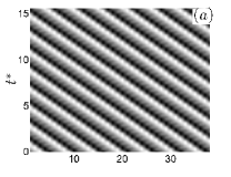
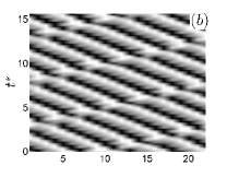
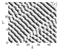
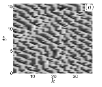
Figure 1: Space-time plots of $X_{k}(t)$ for 15 time units after $t=5.1\times 10^{5}$ indicated by $t^{*}$. Dark regions are large values and light regions are small values: (a) $N=38$, $F=5$, periodic dynamics; (b) $N=22$, $F=5$, low-dimensional chaotic dynamics; (c) $N=47$, $F=5$, chaotic dynamics; (d) $N=38$, $F=10$, chaotic dynamics.

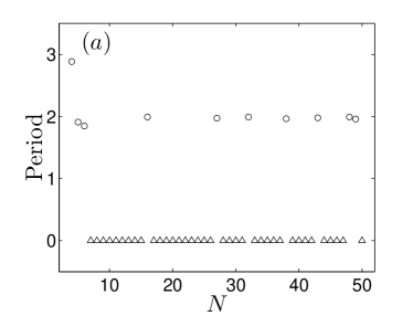
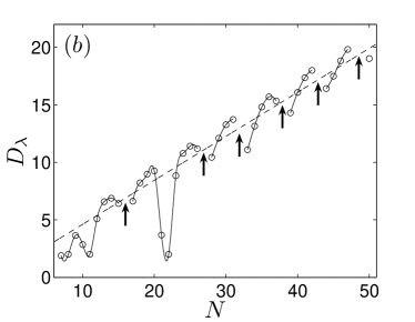
Figure 2: The variation of the dynamics with system size $N$ for $F=5$. (a) Periodic dynamics (circles) where the ordinate indicates period duration and chaotic dynamics (triangles). Chaotic dynamics have been assigned an arbitrary period of ‘$0$’ to fit on a single plot. (b) Deviations from extensivity illustrated by the variation of $D_{\lambda}$ with $N$. The circles are simulation results and the solid lines are to guide the eye. The maximum value of $\Delta D=0.77$ occurs for $N=22$, for $N\geq 27$ the maximum deviation is $\Delta D=0.17$. The arrows indicate windows of periodic dynamics. The error in these calculations is $\sim 10^{-2}$ as determined by the standard deviation of $D_{\lambda}$ using $10$ different initial conditions at each $N$.

We now compare these results based upon the use of Lyapunov exponents with what is found by analyzing the spatial and temporal characteristics of the patterns. Analysis of the patterns are of particular interest because these measurements are often available in experiment whereas the Lyapunov exponent based diagnostics are not. Figure 3(a) shows the variation of the correlation time $\xi_{t}$ with increasing system size. The correlation time is computed from

$$\left<X_{k}(0)X_{k}(t)\right>\sim e^{-t/\xi_{t}}$$ (8)

where $\left<X_{k}(0)X_{k}(t)\right>$ is the autocorrelation of the $k$th variable. The results shown are the time average value of the correlation time for the variable $X_{1}(t)$ in the periodic lattice. Each data point is also averaged over simulations begun from 10 different random initial conditions. The open symbols represent chaotic dynamics and the filled symbols represent periodic dynamics. The results exhibit a scatter about the mean value of $\xi_{t}=0.162$ with a coefficient of variation of 9.6% (defined as the standard deviation divided by the mean). The results indicate that the time dynamics remain relatively constant as the system size increases.

To quantify the spatial variation of the pattern we have computed the average pattern wavelength $\xi_{L}$ with increasing system size as illustrated in Figure 3(b). The wavelength is computed in Fourier space using the location of the largest peak at small wavenumber to capture the size of the basic wave structure and is averaged over all time for each initial condition. Computation of the two-point spatial correlation length is difficult due the lack of an exponential decay in the correlation functions for the parameters we have explored. For smaller systems $N\lesssim 10$ the deviations are largest whereas for $N>10$ the wavelength varies about an average value of $\xi_{\lambda}\approx 5.2$ lattice spacings. For the chaotic solutions, the fluctuations about the average value over the 10 different initial conditions yields a coefficient of variation of approximately $14\%$. For the periodic dynamics the wavelength of the periodic states were nearly identical to the precision of our calculations over the different initial conditions.

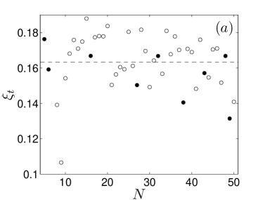
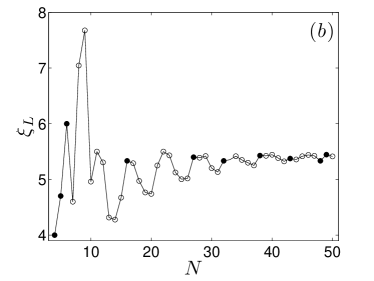
Figure 3: The temporal and spatial features of the patterns for $F=5$. (a) The variation of the average correlation time $\xi_{t}$ with system size $N$. The dashed line is the average value of $\xi_{t}$. (b) The variation of the pattern wavelength $\xi_{L}$ with system size. In both panels open symbols represent chaotic dynamics and filled symbols represent periodic dynamics.

Our space-time diagnostics indicate that with increasing system size the dynamics tend toward a state where $\xi_{t}\approx 0.16$ and $\xi_{L}\approx 5.2$. The wavelength of the pattern in the large system limit is $\xi_{L}\approx 2\xi_{\delta}\approx 2.2\xi_{0}$ indicating that each wavelength of the pattern contains approximately 2 chaotic degrees of freedom on average. In this case, it is useful to compare the deviations from extensivity with the variations in the wavelength of the patterns for increasing system size.

The variation of $\xi_{L}$ about its mean value is quite similar to what is found for the deviations from extensivity $\Delta D$ as illustrated in Fig. 4. We plot the variation of the normalized wavelength $\tilde{\xi}_{L}$ and the normalized deviations from extensivity $\Delta\tilde{D}$ with the system size. The constant normalization factors are chosen such that the normalized wavelength and deviation from extensivity equal unity for $N=25$ allowing both curves to be shown on a single plot. The circles are results for the wavelength of the pattern where solid symbols indicate periodic dynamics, open symbols represent chaotic dynamics, and the solid line is a curve fit. The dashed line and the square symbols represent the deviations from extensivity. Gaps in the dashed line occur for system sizes exhibiting periodic dynamics.

Figure 4 illustrates a correlation between the pattern wavelength and the deviation from extensivity. The general trend is that both the fractal dimension and the pattern wavelength increase with increasing system size until the pattern adjusts by adding an additional wave structure to the periodic lattice effectively reducing the average wavelength of the pattern. With the addition of the wave structure the dynamics are periodic and the fractal dimension vanishes. A similar trend is seen in the work of Fishman et al. Fishman and Egolf (2006) where periodic dynamics were found for system sizes where the deviation from extenisivity was predicted to be a minimum for the one-dimensional complex Ginzburg-Landau equation.

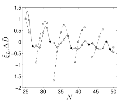
Figure 4: A comparison of the variation in the normalized pattern wavelength $\tilde{\xi}_{L}$ and the normalized deviation from extensivity $\Delta\tilde{D}$ for $F=5$ and $N\geq 25$. The constant normalization factor is chosen such that $\Delta\tilde{D}$ and $\tilde{\xi}_{L}$ each equal unity for $N=25$ allowing both curves to fit on a single plot. The wavelength results are given by the circles and the solid line (open symbols are chaotic dynamics, filled symbols are periodic dynamics). The deviations from extensivity are shown by the square symbols and the dashed line where gaps indicate regions of periodic solutions. In both cases the lines are curve fits to guide the eye.

III.1.2 Intermediate External Forcing, $F=10$

We next explore the dynamics for a larger value of the forcing $F=10$ over the range of system sizes $5\leq N\leq 50$. For each system size we have performed 50 independent numerical simulations starting from different random initial conditions. Each simulation was allowed to continue until $t=5\times 10^{5}$ and in computing our results we only used data in in the time interval $3\times 10^{5}\leq t\leq 5\times 10^{5}$ to ensure the decay of all transients and in order to gather good statistics. We found chaotic dynamics at every system size and for each random initial condition. A representative space-time plot for our results is shown in Fig. 1(d) for the case of $N=38$. The patterns consist of distorted wave structures traveling from right to left.

The spectra of Lyapunov exponents are shown in Fig. 5(a) for six different values of system size. The results are normalized by $N$ and for extensive chaos the spectra collapse onto a single curve as expected. The solid line is the average of the results for the different system sizes shown. The variation of the summation of the exponents with the number of exponents is illustrated in Fig. 5(b) for the case of $N=40$. The solid line is a 6th order polynomial curve fit through the average values of the data. The fractal dimension is indicated by the vertical dashed line at the location where the summation vanishes.

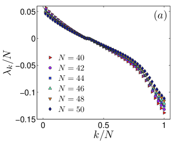
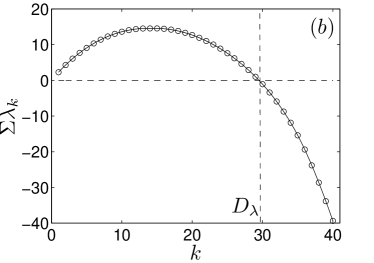
Figure 5: (color online) (a) The variation of the Lyapunov exponents $\lambda_{k}/N$ with $k/N$ for $k=1,\ldots,N$ where $N$ is the system size and $F=10$. The solid line is the average value using all of the data. (b) The variation of the summation of the exponents with $k$ for $F=10$ and $N=40$. The fractal dimension $D_{\lambda}$ is the value where the summation vanishes. The solid line is a 6th order polynomial curve fit and the fractal dimension $D_{\lambda}$ is shown by the vertical dashed line.

The variation of the fractal dimension with system size is shown in Fig. 6. Figure 6(a) illustrates the variation of $D_{\lambda}$ with $N$ where the symbols represent the average value over the 50 different initial conditions. An estimate of the error in these calculations is the standard deviation of the values of the dimension at each system size. Using this, the error is found to be quite small with a magnitude of $\sim 10^{-5}$ over the entire range of system sizes. The solid line is a linear curve fit through the data points indicating extensivitiy. This yields a value of $D_{\text{ext}}$ for any system size $N$ and using Eq. (2) yields a value of the natural chaotic length scale of $\xi_{\delta}=1.35$. It is important to point out that since $\xi_{\delta}>1$, incremental changes in $N$ by adding a single lattice site allow the variation in the fractal dimension to be observed for changes in system size that are smaller than the chaotic length scale.

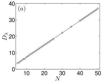
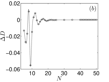
Figure 6: The variation of the dynamics with the system size for $F=10$. (a) The variation of $D_{\lambda}$ with $N$, the solid line is a linear curve fit through the data indicating extensive chaos. For $N=4$ the dynamics are periodic and are not included in the curve fit. (b) The variation of the deviation from extensivity $\Delta D$ with $N$. The circles are results from numerical simulation and the solid line is a curve fit to guide the eye. The deviations from extensivity are on the order of 5% and decreases with increasing $N$. The fluctuations about the average values shown in each panel, as determined from the standard deviation of results from 50 different initial conditions, is on the order of $\sim 10^{-5}$.

The deviations of the fractal dimension about extensivity $\Delta D$ are shown in Fig. 6(b) where we have used Eq. (7) and the solid line is to guide the eye. The magnitude of the deviation from extensivity for $N\leq 25$ is $\sim 5\%$ at its largest value and tends towards zero with increasing $N$. Error bars are included and, over the entire range of system sizes, have a magnitude on the order of $\sim 10^{-5}$ which is 3 orders of magnitude smaller than the absolute values of $\Delta D$. Due to the very small magnitude of our error bars we can discern these deviations in the fractal dimension from extensivity for all values of the system size. This suggests that the deviations from extensivity are not entirely finite-size effects and are inherent to the underlying chaotic dynamics. For the larger system sizes $40\leq N\leq 50$ the magnitude of the deviations from extensivity reduce to $\Delta D\approx 10^{-5}$. We note that over this range the magnitude of the error is on the order of $\sim 10^{-6}$ and these small deviations are still an order of magnitude larger than the error bars.

Figure 6(b) illustrates that the variation of $\Delta D$ with $N$ is non-monotonic in its oscillating decay in amplitude toward extensivity. The previous studies exhibiting deviations from extensivity of O’Hern et al. O’Hern et al. (1996) and Fishman et al. Fishman and Egolf (2006) both observed a rapid monotonic decay towards extensive chaos. At present we do not have a good understanding of the physical origin of the non-monotonicity in our results which is perhaps related to the discrete spatial structure of the Lorenz-96 model.

It is useful to separate these findings into two regimes, a small system regime where $N\leq 25$ and a large system regime where $N\geq 40$. The small system regime includes the onset of extensivity whereas the large systems are extensive. In a more complicated system, one would typically only have access to the deviations from extensivity for the small systems sizes since the deviations are largest in this range. However, this is also the regime where one could expect finite size effects to also be important and complicate the results. The large system limit is expected to be less influenced by these finite size effects and to provide a better estimate of the length scale of a chaotic degree of freedom.

Over these two regimes we find that the wavelength of the deviations varies significantly. To quantify this we compute the zero crossings of $\Delta D$ over each range to estimate the wavelength of oscillation about $D_{\text{ext}}$ given by $\xi_{0}$. For $N\leq 25$ there are 3 wavelengths with values of $(3.3,5.3,1.9)$ that yield an average of $\xi_{0}\approx 3.5$. Assuming each wavelength of $\Delta D$ corresponds to the addition of two degrees of freedom yields $\xi_{0}/2\approx 1.75$ for the size of a single degree of freedom. Comparison of this length with the natural chaotic length scale yields that the size of a single degree of freedom is approximately $1.3\xi_{\delta}$. The large spread in the values of the wavelengths suggests some competition with pattern selection mechanisms.

In the large system limit $N\geq 40$ there are 4 wavelengths characterizing the deviations from extensivity with values $(1.7,1.7,2.6,2.3)$ yielding an average value of $\xi_{0}\approx 2$. The magnitude and variation of the wavelengths are smaller than what was found for the smaller systems. Using the same arguments as before yields that the size of a single degree of freedom is $\xi_{0}/2\approx 1$. Comparison with the natural chaotic length scale yields that a single degree of freedom is $0.74\xi_{\delta}$. As in the case of $F=5$ the results yield that $\xi_{0}/2\approx\xi_{\delta}$ suggesting that the natural chaotic length scale and the wavelength of the deviations from extensivity are related.

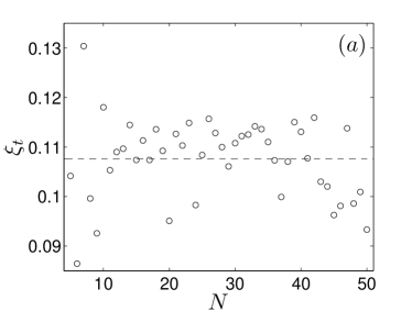
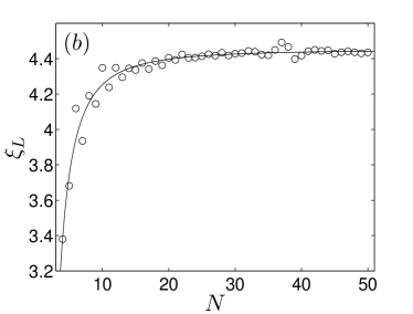
Figure 7: The temporal and spatial characteristics of the patterns for $F=10$. (a) The variation of the average correlation time $\xi_{t}$ with system size $N$. The dashed line is the average value of $\xi_{t}$. (b) The variation of the average pattern wavelength $\xi_{L}$ with system size. The solid line is a curve fit of the form $\xi_{L}=4.45-13.6N^{-1.83}$.

In order to better characterize the patterns we have also computed characteristic time and length scales describing their dynamics. Our motivation is to provide further insight into the transition between the small and large system limits in order to separate finite size effects from dynamical effects related to extensivity. We are also interested in quantifying any relationship between the Lyapunov based diagnostics and the pattern dynamics. Figure 7(a) shows the variation of the average correlation time $\xi_{t}$ with $N$ over 50 different initial conditions. The time dynamics are noisy and the correlation time has an average value of approximately $\xi_{t}\approx 0.11$ (indicated by the dashed line). The time dynamics are faster than what was found for $F=5$ as expected for the increased value of the forcing term.

Figure 7(b) illustrates the variation in the average wavelength of the patterns with $N$ over the different initial condtions. The wavelength variation shows two regions of interest. For small system sizes $N\lesssim 20$ the pattern wavelength increases rapidly. For larger systems the wavelength remains relatively constant with an average value of $\xi_{\lambda}\approx 4.5$. The region of increasing wavelength corresponds to system sizes where the pattern selection is affected significantly by the size of the domain. This corresponds roughly with the region where the fractal dimension is approaching extensivity in Fig. 6(b). These trends are well captured by a power-law, the solid line in the figure is a curve fit through the data of the form $\xi_{L}=4.45-13.6N^{-1.83}$. The fluctuations of the wavelength about the mean value for these chaotic states yields a coefficient of variation of approximately $30\%$.

These results suggest that our measurements of the deviations in the fractal dimension for the large system limit are quantifying the chaotic dynamics in a regime that is not strongly affected by finite size effects. Our space-time diagnostics indicate that the pattern dynamics, in the large system limit, have temporal variations with $\xi_{t}=0.106$ and a spatial wavelength on the order of $\xi_{L}=4.45$. In this case, $\xi_{L}=3.3\xi_{\delta}$ indicating that a wavelength of the pattern contains, on average, 3.3 chaotic degrees of freedom. A more detailed exploration of the relationship between $\xi_{L}$ and $\xi_{\delta}$ for increasing values of the forcing $F$ will be explored in the following section.

III.2 Variation of the Fractal Dimension with Forcing

In the previous sections we have considered the large system limit, defined as the limit where the chaotic degrees of freedom are much smaller than the system size. This was achieved by holding the external forcing $F$ fixed while the system size $N$ was increased. This is the typical manner to study spatiotemporal chaos and has been referred to as the ‘spatiotemporal chaos’ limit Cross and Hohenberg (1993). For example, in a Rayleigh-Bénard convection experiment this could be accomplished by holding the Rayleigh number constant while increasing the aspect ratio of the convective domain.

However, it is also possible to explore the large system limit by keeping the system size fixed while increasing the external forcing. This has been referred to as the strong driving or ‘strong turbulence’ limit Cross and Hohenberg (1993). In this case, it is expected that the chaotic degrees of freedom will become smaller with increasing forcing to yield the large system limit. In a Rayleigh-Bénard convection experiment this would be accomplished by increasing the Rayleigh number in a convection domain of fixed size. It has been conjectured that the fractal dimension will also exhibit a power-law dependence with respect to the value of the forcing Cross and Hohenberg (1993).

We have explored this strong driving limit in the Lorenz-96 model by performing a series of simulations for increasing values of $F$ while the system size $N$ is held constant. We studied 6 values of the forcing over the range $5\leq F\leq 30$. For any particular value of $F$ we performed 10 numerical simulations starting from different random initial conditions and allowed the simulation to run for $5\times 10^{5}$ time units to ensure good statistics. We computed these results for 5 different system sizes where $15\leq N\leq 35$.

It is more convenient to discuss these results using the intensive dimension density,

$$\delta_{\lambda}=\frac{D_{\lambda}}{N}.$$ (9)

The variation of the dimension density with external forcing is shown in Fig. 8. Each symbol is the average value of the 10 simulations from different random initial conditions. The standard deviation of the results are $\sim 10^{-5}$ and have not been included as error bars due to their small magnitude.

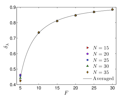
Figure 8: (color online) The variation of the dimension density $\delta_{\lambda}$ with the forcing $F$ and system size $N$. The results are for 5 different system sizes indicated in the legend. The symbols are simulation results and the solid line is a power-law curve fit through the average value of the data. Each symbol is the average value from results computed using 10 different initial conditions. The standard deviation of these results for each symbol is $\sim 10^{-5}$.

The dimension density exhibits power-law behavior and the results for different values of $N$ collapse onto a single power-law curve given by,

$$\delta_{\lambda}(F)=a+bF^{-\alpha}$$ (10)

where $a=0.93$, $b=-4.03$, and $\alpha=1.32$. The power-law curve fit is given by the solid line. The coefficient $a$ in this case is the predicted value of the dimension density for external forcing of infinite magnitude $\delta_{\infty}$. The scatter in the results is quite small for all values of $F$ explored with the largest deviations occurring at the smallest value of the forcing. The coefficients of the power-law are also collected in Table 2 for reference.

The inverse of the dimension density is simply the natural chaotic length scale $\xi_{\delta}=\delta_{\lambda}^{-1}$. Therefore Fig. 8 can be used to illustrate the manner in which the chaotic length scale decreases with increasing forcing. This is a spatially discrete system with $N$ degrees of freedom and the theoretical limit for the dimension density is $\delta_{\lambda}=1$ corresponding to a chaotic length scale of a single lattice spacing $\xi_{\delta}=1$. Using our results for $\delta_{\infty}$ yields a value of $\xi_{\delta}=1.08$ for the chaotic length in the limit of infinite forcing. This is in contrast to a fluid system described by partial differential equations with an infinite number of degrees of freedom. It is interesting to note that the variation of the fractal dimension with the degree of external forcing has been explored numerically for turbulent Rayleigh-Bénard convection to yield a linear dependence Sirovich and Deane (1991).

We now compare several measures of characteristic time and length scales for increasing values of the magnitude of external forcing. Both the temporal and spatial scales decrease with increasing forcing as expected. The variation of these scales are well described by a power-law of the functional form given by Eq. (10). The variation of the inverse leading order Lyapunov exponent and the correlation time are shown in Fig 9. The symbols are results from our simulations for each value of $F$. The value of $\lambda_{1}^{-1}$ yields a time scale related to the predictability of the system. The solid line in Fig 9(a) is a power-law curve fit using the values shown in Table 2. The inverse Lyapunov exponents have been scaled by the system size $N$ so that all data can be represented on a single plot. The value of $a=0.15$ represents $\lambda_{1}^{-1}/N$ for infinite $F$.

Figure 9(b) illustrates the variation of the average correlation time $\xi_{t}$ with increased forcing and over the 10 different initial conditions for a large system with $N=35$. The solid line is the power-law curve fit using the values of Table 2. The fluctuations of the correlation time about the mean value over the different initial conditions is quite noisy and yields a coefficient of variation of 7.7%. In the limit of infinite forcing the average correlation time $\xi_{t}\approx 0$. Our results suggest that the predictability decreases faster than the correlation time indicating the possibility of at least two different time scales.

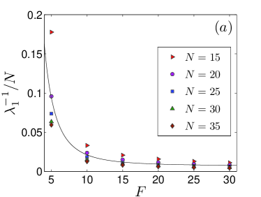
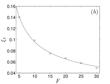
Figure 9: The variation of two characteristic time scales with external forcing $F$. (a) The variation of the normalized inverse of the leading order Lyapunov exponent $\lambda_{1}^{-1}/N$. Data are shown for 5 different system sizes as indicated in the legend. The solid line is a curve fit through the data of the form $\lambda_{1}^{-1}/N=0.007+5.9F^{-2.6}$. (b) The variation of the average correlation time $\xi_{t}$ with $F$ for a system size of $N=35$. The symbols are results from simulation and the solid line is the power-law $\xi_{t}=0.35F^{-0.56}$ .

	$a$	$b$	$\alpha$
$\delta_{\lambda}$	0.93	- 4.03	1.32
$\lambda_{1}^{-1}/N$	0.007	5.9	2.6
$\xi_{t}$	$0$	0.35	0.56
$\xi_{\delta}$	1.12	39.74	2.2
$\xi_{L}$	4.38	-290.8	3.5

Table 2: The coefficients describing power-law trends in the data from numerical simulations exploring the chaotic patterns as the magnitude of the external forcing is varied. The first row is for the dimension density $\delta_{\lambda}$, the next two rows describe temporal scales given by the inverse leading order Lyapunov exponent $\lambda_{1}^{-1}$ and correlation time $\xi_{t}$, and the final two rows are spatial scales given by the natural chaotic length scale $\xi_{\delta}$ and the pattern wavelength $\xi_{L}$. The functional form of the power-law used is $a+bF^{-\alpha}$.

The pattern wavelength and the chaotic length scale both decrease with a power-law variation given by Eq. (10) for increasing values of the magnitude of the external forcing. The coefficients of the power-law variation are given in Table 2. The variation of these length scales is shown in Fig. 10(a). The pattern wavelength is represented using square symbols and the natural chaotic length scale is represented using circle symbols. The length scales have been normalized by their magnitude at $F=5$ to facilitate a comparison using a single plot. The normalized length scales are referred to as $\tilde{\xi}_{L}$ and $\tilde{\xi}_{0}$, respectively. The coefficient of variation, over the different initial conditions, for the chaotic length scale is quite small $\sim 0.01\%$ whereas the pattern wavelength measurements are quite noisy with a coefficient of variation of $\sim 31\%$.

It is clear that the natural chaotic length scale decreases more rapidly than the pattern wavelength. The ratio of these two length scales yields an estimate for the number of chaotic degrees of freedom per pattern wavelength and is shown in Fig. 10. For small values of the forcing there are approximately 2 degrees of freedom per wavelength which increases to nearly 4 degrees of freedom per wavelength for large values of the forcing. The separation of these two length scales suggests that for larger values of the external forcing significant contributions to the overall disorder are from sub-wavelength structures in the pattern dynamics. A clear signature of the sub-wavelength chaotic degree of freedom was not found using our spatial diagnostics.

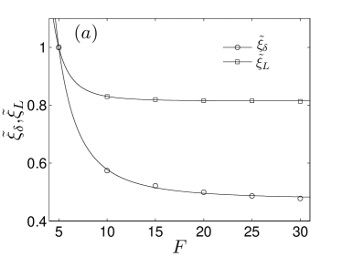
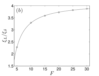
Figure 10: The variation of two characteristic spatial scales with external forcing $F$ for a system size of $N=35$. (a) The normalized natural chaotic length scale $\tilde{\xi}_{\delta}$ (circles) and the normalized pattern wavelength $\tilde{\xi}_{L}$ (squares). The normalization factors used are the respective values of $\xi_{\delta}$ and $\xi_{L}$ at $F=5$. The power-law curve fits for the unscaled length scales are $\xi_{\delta}=1.12+39.74F^{-2.2}$ and $\xi_{L}=4.38-290.8F^{-3.5}$. (b) The ratio $\xi_{L}/\xi_{\delta}$ yields an estimate for the number of chaotic degrees of freedom per pattern wavelength.

IV Conclusions

Using a phenomenological model relevant to fluid convection and the atmosphere we have shown that the variation of the fractal dimension with system parameters can provide physical insights into fundamental features of high-dimensional chaos. We have used the fractal dimension to provide an approximate value of the number of chaotic degrees of freedom in the system and to estimate length scales describing the underlying chaotic dynamics.

If one considers only the space-time diagnostics of the correlation time and pattern wavelength the results exhibit significant fluctuations despite the use of very long-time simulations for numerous initial conditions. This is in contrast to what is found when using the fractal dimension and suggests the possibility of features of the dynamics that have yet to be quantified in detail. Our results indicate that the length scale describing the deviations from extensivity is approximately equal to the natural chaotic length scale which suggests the possibility of important spatial structures that contribute significantly to the chaotic dynamics. Clearly identifying such features, and relating them to experimentally accessible quantities, remains an important open challenge in the characterization of systems driven far-from-equilibrium.

For systems of small size with low values of external forcing we find very complicated dynamics with windows of periodic and chaotic dynamics. This is similar to what has been found both numerically Paul et al. (2001) and experimentally Bodenschatz et al. (2000) in fluid systems such as Rayleigh-Bénard convection. For intermediate forcing, extensive chaos emerges with the important feature of significant deviations from extensivity for incremental changes in system size. Our results suggest that such behavior may be present in experimentally accessible fluid systems. The ratio of our measured length scales, such as the ratio of the chaotic length scale $\xi_{\delta}$ to the wavelength of the deviations from extensivity $\xi_{0}$ do not yield integer values as found for the 1D complex Ginzburg-Landau equation Fishman and Egolf (2006). This is perhaps also due in part to the discrete spatial nature of the Lorenz-96 model.

The variation of the fractal dimension with external forcing yields insights into the manner in which the chaotic length scale decreases as the strong driving limit is approached. In the case of increasing system size while holding the forcing fixed, extensive chaos occurs when the exponent relating the dimension and system size is equal to the number of spatially extended directions. However, a similar theoretical understanding of the growth in the fractal dimension with increased forcing remains an open challenge. The fact that our results are independent of system size is promising and suggests that perhaps this is an underlying feature of some generality. It is anticipated that our results will be useful in guiding future efforts to explore the extensive chaos of experimentally accessible systems.

Acknowledgments: The computations were conducted using the resources of the Advanced Research Computing center at Virginia Tech and the research was supported by NSF grant no. CBET-0747727.

References

- Cross and Hohenberg (1993) M. C. Cross and P. C. Hohenberg, Rev. Mod. Phys. 65, 851 (1993).
- Lorenz (1968) E. N. Lorenz, Tellus XXI, 289 (1968).
- Bodenschatz et al. (2000) E. Bodenschatz, W. Pesch, and G. Ahlers, Annu. Rev. Fluid Mech. 32, 709 (2000).
- Bees and Hill (1997) M. A. Bees and N. A. Hill, J. Exp. Biol. 200, 1515 (1997).
- Bar and Eiswirth (1993) M. Bar and M. Eiswirth, Phys. Rev. E 48, R1635 (1993).
- Nugent et al. (2004) C. R. Nugent, W. M. Quarles, and T. H. Solomon, Phys. Rev. Lett. 93, 218301 (2004).
- Abarbanel (1996) H. D. I. Abarbanel, Analysis of Observed Chaotic Data (Springer, 1996).
- Wiggins (2003) S. Wiggins, Introduction to applied nonlinear dynamical systems and chaos (Springer, New York, 2003).
- Lorenz (1963) E. N. Lorenz, J. Atmos. Sci 20, 130 (1963).
- Robinson (1995) J. Robinson, Chaos 5, 330 (1995).
- Yang et al. (2009) H. Yang, K. Takeuchi, F. Ginelli, H. Chatè, and G. Radons, Phys. Rev. Lett. 102, 074102 (2009).
- Ott (1993) E. Ott, Chaos in dynamical systems (Cambridge University Press, New York, 1993).
- Ruelle and Eckmann (1985) D. Ruelle and J. P. Eckmann, Rev. Mod. Phys. 57, 617 (1985).
- Farmer et al. (1983) J. D. Farmer, E. Ott, and J. A. Yorke, Physica D 7, 153 (1983).
- Ruelle (1982) D. Ruelle, Commun. Math. Phys. 87, 287 (1982).
- O’Hern et al. (1996) C. S. O’Hern, D. A. Egolf, and H. S. Greenside, Phys. Rev. E 53, 3374 (1996).
- Manneville (1985) P. Manneville, Lecture Notes in Pysics 230, 319 (1985).
- Fishman and Egolf (2006) M. P. Fishman and D. A. Egolf, Phys. Rev. Lett. 96, 054103 (2006).
- Tajima and Greenside (2002) S. Tajima and H. S. Greenside, Phys. Rev. E 66, 017205 (2002).
- Xi et al. (2000) H. W. Xi, R. Toral, J. D. Gunton, and M. I. Tribelsky, Phys. Rev. E 62, R17 (2000).
- Egolf et al. (2000) D. A. Egolf, I. V. Melnikov, W. Pesch, and R. E. Ecke, Nature 404, 733 (2000).
- Paul et al. (2007) M. R. Paul, M. I. Einarsson, P. F. Fischer, and M. C. Cross, Phys. Rev. E 75, 045203 (2007).
- Lorenz (1996) E. N. Lorenz, Proc. Seminar on Predictability 1, 1 (1996).
- Lorenz and Emanuel (1998) E. N. Lorenz and K. A. Emanuel, J. Atmos. Sci. 655, 399 (1998).
- Boffetta et al. (2002) G. Boffetta, M. Cencini, M. Falcioni, and A. Vulpiani, Phys. Rep. 356, 367 (2002).
- Ott et al. (2004) E. Ott, B. R. Hunt, I. Szunyogh, A. V. Zimin, E. J. Kostelich, E. Kalnay, D. J. Patil, and J. A. Yorke, Tellus 56, 415 (2004).
- Pazó et al. (2008) D. Pazó, I. G. Szendro, J. López, and M. A. Rodríguez, Phys. Rev. E 78, 016209 (2008).
- Wolf et al. (1985) A. Wolf, J. B. Swift, H. L. Swinney, and J. A. Vastano, Physica D 16, 285 (1985).
- Sirovich and Deane (1991) L. Sirovich and A. E. Deane, J. Fluid Mech. 222, 251 (1991).
- Paul et al. (2001) M. R. Paul, M. C. Cross, P. F. Fischer, and H. S. Greenside, Phys. Rev. Lett. 87, 154501 (2001).