An ab initio method for locating characteristic potential energy minima

Abstract

It is possible in principle to probe the many–atom potential surface using density functional theory (DFT). This will allow us to apply DFT to the Hamiltonian formulation of atomic motion in monatomic liquids [Phys. Rev. E 56, 4179 (1997)]. For a monatomic system, analysis of the potential surface is facilitated by the random and symmetric classification of potential energy valleys. Since the random valleys are numerically dominant and uniform in their macroscopic potential properties, only a few quenches are necessary to establish these properties. Here we describe an efficient technique for doing this. Quenches are done from easily generated “stochastic” configurations, in which the nuclei are distributed uniformly within a constraint limiting the closeness of approach. For metallic Na with atomic pair potential interactions, it is shown that quenches from stochastic configurations and quenches from equilibrium liquid Molecular Dynamics (MD) configurations produce statistically identical distributions of the structural potential energy. Again for metallic Na, it is shown that DFT quenches from stochastic configurations provide the parameters which calibrate the Hamiltonian. A statistical mechanical analysis shows how the underlying potential properties can be extracted from the distributions found in quenches from stochastic configurations.

I Introduction

The potential energy surface underlying the motion of a monatomic liquid is composed of intersecting valleys in the many–atom configuration space. In Vibration–Transit (V-T) theory, the atomic motion is described by vibrations within a single valley, interspersed by transits, which carry the system across intervalley intersections Wallace (1997); Chisolm and Wallace (2001). The pure vibrational motion is described by a tractable Hamiltonian which accounts for the dominant part of the liquid’s thermodynamic properties. The remaining transit contribution is complicated but small. The vibrational Hamiltonian is calibrated by potential parameters evaluated at local minima (called structures) of the potential surface. These have been previously evaluated for a model of liquid Na based on an interatomic pair potential De Lorenzi-Venneri and Wallace (2007). Our goal now is to introduce first principles electronic structure calculations within density functional theory (DFT) to calculate the structural and vibrational parameters of the V-T Hamiltonian.

In recent years, DFT has been used successfully in liquid studies to support the development of ab initio Molecular Dynamics (MD). The original Car–Parrinello method Car and Parrinello (1985) was successfully applied to the melting of Si Sugino and Car (1995). Calculations of the MD trajectory on the adiabatic (electronic ground state) potential surface have been performed for a broad spectrum of elemental liquids Kresse and Hafner (1993a, b); Kresse (2002). This work has provided accurate and physically revealing results for Al de Wijs et al. (1998), Fe Alfè et al. (2000), and Ge Chai et al. (2003). The techniques we employ to calculate the supercell ground state energy and Hellmann–Feynman forces are quite similar to those of Kresse et al. Kresse and Furthmüller (1996). On the other hand, rather than proceed to MD calculations, our objective is to calibrate the (dominant) vibrational part of the liquid dynamics Hamiltonian from properties of local potential minima. We believe that the Hamiltonian formulation will usefully complement ab initio MD in the study of dynamical properties of liquids.

The procedure of quenching a system to its potential energy minima was introduced by Stillinger and Weber Stillinger and Weber (1982); Weber and Stillinger (1984); Stillinger and Weber (1984), and has become a valuable technique for studying systems with interatomic potentials. The traditional method is to quench to many structures from an equilibrium MD trajectory, and then use statistical mechanics to extract the underlying statistical properties of the potential surface Heuer and Büchner (2000); Sciortino et al. (1999). In V-T theory, however, we need very few structures—in principle only one for a given liquid at a given volume. Hence the traditional procedure for finding structures is inefficient, as a large number of MD iterations is required to bring the system initially to equilibrium as well as to avoid unwanted correlations between quenches. The problem is especially severe for DFT, where each iteration requires a converged total energy calculation, which is computationally very costly.

We propose a simpler and more efficient method to probe the underlying potential landscape. Rather than quench from equilibrium MD configurations, we quench from configurations that are independent of interatomic interactions, and very fast to generate. Our purpose here is to demonstrate two properties of this quench method: that it is capable of producing the entire distribution of potential energy minima, and when used with DFT it can achieve our goal of ab initio calibration of the Hamiltonian.

To perform the calibration, we will interpret structural data via the original hypothesis of V-T theory Wallace (1997): The potential energy valleys are classified as random and symmetric. The random valleys numerically dominate the liquid statistical mechanics as $N\rightarrow\infty$, and they all have the same potential energy properties as $N\rightarrow\infty$; hence any one such valley may be used to calibrate the Hamiltonian. The symmetric valleys have a broad range of potential energy properties, but make an insignificant contribution to the liquid statistical mechanics as $N\rightarrow\infty$. This hypothesis has been verified for the pair potential model of liquid Na at $N=500$ De Lorenzi-Venneri and Wallace (2007), and work in progress extends this verification to $N=4000$ Holmström et al. (2009).

The quench calculations are carried out for metallic Na at the density of the liquid at melt, using our model interatomic potential, and also using DFT. The Na potential was derived in pseudopotential perturbation theory, with an added Born–Mayer repulsion, and was calibrated from experimental crystal data at zero temperature and pressure Wallace (1968). The potential has since been shown to give excellent results for a broad range of experimental properties of crystal and liquid Na (for a partial summary, see Wallace (2002)). While there is no doubt DFT will provide accurate total energy results, we shall still need to verify that DFT quenches arrive at random structures, not symmetric ones. This verification will be accomplished with the aid of the Na interatomic potential results.

Our application of DFT to liquid dynamics theory is being pursued for a number of nearly–free–electron metals and transition metals. A preliminary report has been presented on results for Na and Cu Bock et al. (2008). We have not attempted to study elemental liquids whose equilibrium configurations are influenced by molecular bonding. Examples are As, Se, and Te, which have strong and weak bonds, and Ge, whose liquid structure shows a contribution from covalent crystal bonds. This anisotropic bonding will complicate the random structures underlying the motion in such liquids. This complication remains beyond the scope of the present work. Moreover, since we have not yet presented structural data for other liquid metals, the present conclusions are strictly valid only for liquid Na. The results are expected to apply to many elemental liquids, perhaps all of them, but this extension is not demonstrated here.

We consider a system of atoms in a cubic box with periodic boundary conditions. We construct configurations in which the nuclei are distributed uniformly over the box, within a constraint limiting the closeness of approach of any pair. These are called constrained stochastic, or simply stochastic, configurations. The procedure is described in Sec. II, and the spatial uniformity is verified by means of pair distribution functions. In Sec. III, our twofold purpose is addressed by two separate quench studies. In Sec. III.1, the Na pair potential is used to quench both equilibrium MD configurations and stochastic configurations. Comparison of the results will validate the use of stochastic configurations. In Sec. III.2, DFT is used to quench Na from stochastic configurations. Comparison of the results with pair potential results will confirm that the DFT structures are random and therefore calibrate the Hamiltonian. In Sec. IV, relations are derived between quenched distributions and the densities of states in the underlying potential energy surface. This analysis provides the statistical mechanical framework for interpreting results of the present quench technique. Our conclusions are summarized in Sec. V.

II Generating stochastic configurations

Only minimal information is required to generate stochastic configurations: the number of atoms $N$ and the system volume $V$, plus a distance of closest approach which is described below. Nothing of boundary conditions or the system potential has to be specified; however, after the stochastic configuration is constructed, for all further calculations periodic boundary conditions are used.

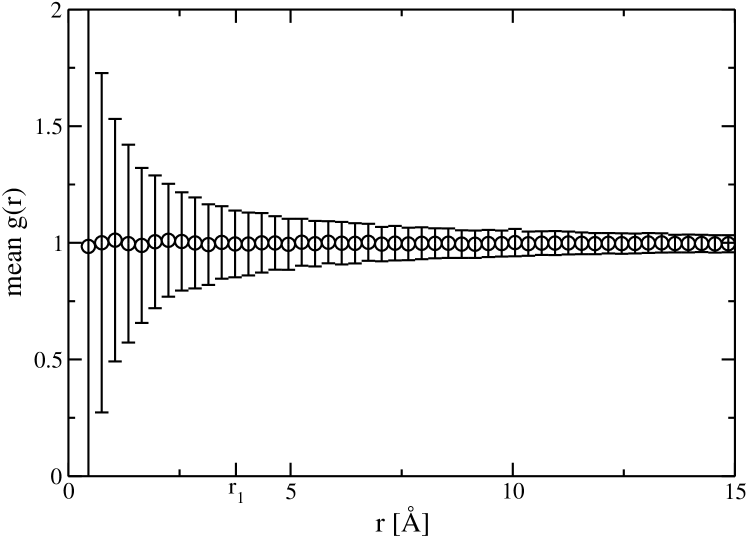
Figure 1: Mean and standard deviation of the pair distribution functions $g(r)$ for 1000 stochastic configurations of $N=500$ atoms. The error bars indicate the standard deviation per histogram bin. The center of the nearest neighbor peak in $g(r)$ for the quenched configuration of Na, shown in Fig. 6, is at $r_{1}=3.77$ Å.

For a cubic cell with volume $V$, we construct a configuration by choosing the particle coordinates at random over the cell. Randomness is important, as we shall use it in Sec. IV to determine the statistical weight factors for stochastic configurations. Next, a configuration is discarded if any two atoms are closer than a distance $d$. This is done for practical reasons: The self consistent field (SCF) calculation of DFT will not converge if atoms are too close to each other, and the pair potential at very small radii could lead to numerical instabilities in the conjugate gradient method due to the repulsive core. In practice, the excluded space can be very small. For Na we choose $d=0.4$ Å, so the relative excluded space $\left(4\pi/3\right)d^{3}/V_{A}$, where $V_{A}$ is the volume per atom, is only $6.5\times 10^{-3}$. Hence the stochastic configurations are expected to be spatially uniform to a very good approximation.

To test the uniformity of stochastic configurations, we examine their pair distribution functions $g(r)$. The conditional probability density $g(r)$ is constructed as follows: Pick a system atom as central atom and denote its position by $r=0$. Make a set of bins labeled $b=1,2,\cdots$, in the form of concentric shells. Bin $b$ has inner radius $r_{b}$, outer radius $r_{b+1}$, and volume $V_{b}=(4\pi/3)\left(r_{b+1}^{3}-r_{b}^{3}\right)$. The pair distribution function $g(r)$ has histogram $n_{b}\left(V_{A}/V_{b}\right)$, where $n_{b}$ is the number of atoms in bin $b$. Given the small size of $d$ described in the previous paragraph, we expect $g(r)$ to be nonzero even at relatively small radii. It is therefore important to normalize the bin count of bin $b$ with the correct volume of the bin, instead of using the approximate volume $4\pi r_{b}^{2}\Delta r_{b}$ as is often done. The bin contents are then averaged over the choice of each system atom as the central atom. While the bin radii are arbitrary, we usually take either $\Delta r_{b}=r_{b+1}-r_{b}=$ constant or $V_{b}=$ constant.

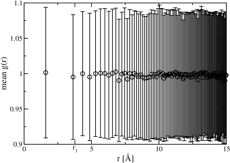
Figure 2: Mean and standard deviation of the pair distribution functions $g(r)$ for 1000 stochastic configurations of $N=500$ atoms. The bins have a constant volume of $V_{b}=(1/8)V_{A}$, where $V_{A}$ is the atomic volume of Na. The center of the nearest neighbor peak in $g(r)$ for the quenched configuration, shown in Fig. 6, is at $r_{1}=3.77$ Å. For this particular binning volume, we have only 2 bins below the nearest neighbor peak.

For Na at $N=500$, we constructed 1000 stochastic configurations and the $g(r)$ histogram for each. With $\Delta r_{b}=$ constant, the mean and the standard deviation of the $g(r)$ histogram are shown in Fig. 1. The blank space at small $r$ is the empty sphere of radius $d$. The scatter at small $r$ reflects the decreasing $V_{b}$ as $r$ decreases, and the corresponding decrease in $n_{b}$. With $V_{b}=$ constant, the mean and standard deviation of the $g(r)$ histogram is shown in Fig. 2. There the distance between points increases as $r$ decreases, but the standard deviation remains nearly constant because $n_{b}$ remains nearly constant. The figures show the uniformity of stochastic configurations for $r>d$, with $d$ being very small compared to the mean nearest neighbor distance.

We also show the distribution of potential energies of the 1000 initial stochastic configurations. The mean of the distribution shown in Fig. 3 is at 3.75 eV/atom, which is considerably higher than the mean potential energy after the quench (see Eq. (1)).

III Properties of the quenched structures

III.1 Validation of quenches from stochastic configurations

Figs. 4 and 5 compare two distributions of $\Phi_{0}/N$, each from 1000 pair potential quenches at $N=500$. Fig. 4 is obtained by steepest–descent quenches from equilibrium MD at 800 K. This figure is an extension of the work reported by De Lorenzi-Venneri and Wallace (2007). Fig. 5 is obtained by conjugate gradient quenches from stochastic configurations. We have verified the equivalence of the two quench techniques for our system; for a related verification, see Chakravarty et al. (2005); Chakraborty and Chakravarty (2006).

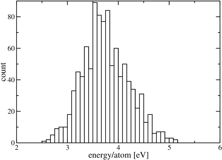
Figure 3: Potential energy distribution of 1000 stochastic configurations of $N=500$ Na atom systems.

In each histogram we see the distinct random and symmetric distributions, consistent with the V-T hypothesis. The random distribution is taken to be the dominant peak, out to where the histogram vanishes on either side. The symmetric structures are interpreted as the isolated parts of the histogram that are located outside the main peak on the low–energy side.

The random distribution is numerically dominant and very narrow. The mean and standard deviation of each random distribution is given by

$$\Phi_{0}/N=\left\{\begin{array}[]{l}-183.29\pm 0.50\mbox{ meV/atom (MD)}\\ -183.37\pm 0.50\mbox{ meV/atom (stochastic)}.\end{array}\right.$$ (1)

Note that the dominant volume–dependent part of the pair potential is omitted here (see Wallace and Clements (1999), Eq. (1.1) and Fig. 1). For this reason, most of the binding energy is missing from the pair potential energies in Eq. (1). The mean value is the most accurate approximation to the thermodynamic limit value that we can make. The standard deviation is the error expected from quenching only once and using that result. If $N$ is increased, the mean value is expected to change slightly in converging to its thermodynamic limit, while the standard deviation goes to zero as $N\rightarrow\infty$. For a physical measure of the difference in mean values, we note that the main contribution to the liquid thermal energy is the classical vibrational contribution $3k_{B}T$, which is 95.90 meV/atom at $T_{m}$. The difference in means is 0.08% of this. Experimental error in the thermal energy of elemental liquids at $T_{m}$ is typically (0.1 - 0.5)%. Hence the two random distributions in Figs. 4 and 5 are identical to better than experimental error.

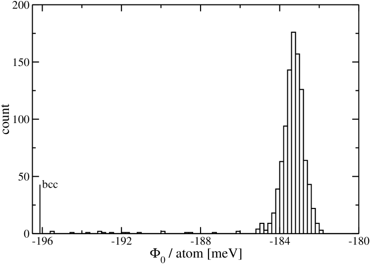
Figure 4: Potential energy distribution of $N=500$ Na atom systems after quenching from 1000 configurations drawn from a molecular dynamics trajectory at 800 K, or $2.16T_{m}$, using a steepest–descent quench method.

Performing so many quenches has allowed us for the first time to see a clear and meaningful distribution of symmetric structures (compare for example De Lorenzi-Venneri and Wallace (2007); Clements and Wallace (1999); Wallace and Clements (1999)). Quenching from equilibrium MD yields 18 symmetric structures out of 1000 quenches, Fig. 4. Quenching from stochastic configurations yields 23 symmetric structures in 1000 quenches, Fig. 5. Very approximately, the symmetric distribution is constant and ranges from the bcc crystal, $\Phi_{0}^{bcc}/N=-196.12$ meV/atom Wallace and Clements (1999), to the lower end of the random distribution. This broad distribution with few structures is consistent with the V-T hypothesis. If $N$ is increased the symmetric distribution width is expected to remain the same, while the relative number of symmetrics is expected to become negligible. In all these properties, the symmetric distributions in Figs. 4 and 5 are the same to statistical accuracy.

III.2 Calibration of the V-T Hamiltonian

In order to calculate ab initio the thermodynamic properties of liquid Na for comparison with experiment, we quenched a stochastic configuration at $V_{A}=41.27$ ų with DFT Bock et al. (2008). The normal mode frequency spectrum $g(\omega)$ was also calculated at this volume. For almost all monatomic liquids, the vibrational motion is nearly classical at $T\geq T_{m}$. This means that the essential information required from $g(\omega)$ is the logarithmic moment of the frequencies, which provides the characteristic temperature $\theta_{0}$. Hence for calculation of thermodynamic properties, the V-T Hamiltonian is calibrated from $\Phi_{0}/N$ for the energy, and $\theta_{0}$ for the entropy. Additional data which automatically accompanies the calculation of $g(\omega)$ will calibrate the Hamiltonian for nonequilibrium statistical mechanics.

The DFT calculation is done with the VASP code VAS , using the projector augmented wave (PAW) method in the generalized gradient approximation (GGA) Blöchl (1994); Kresse and Joubert (1999). The planewave energy cutoff is 101.7 eV, the maximum core radius is 2.5 Å, and the total energy convergence criterion is $10^{-8}$ eV. We use a $\Gamma$–centered Monkhorst–Pack grid Monkhorst and Pack (1976) with 14 $\bm{k}$–points in the irreducible Brillouin zone. The total energy convergence for these parameters was carefully verified. Note that it is the large size of the real–space supercell which allows us to use few $\bm{k}$–points in comparison to the large number (several thousands) needed for crystal metal calculations with small unit cells. The quench is done by nonlinear conjugate gradient method. The system is considered quenched when the energy difference between subsequent configurations is 10^-7 eV or less. The DFT structure is at $N=150$, a number large enough to get potential energy parameters accurate to a few percent, but small enough that convergence properties of the calculations can be studied.

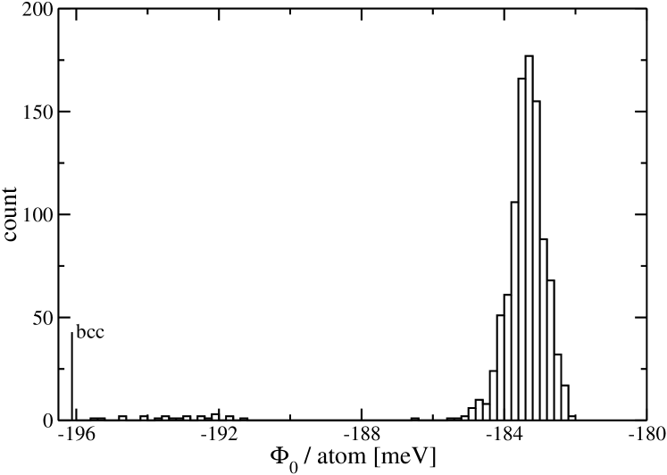
Figure 5: Potential energy distribution of $N=500$ Na atom systems after quenching from 1000 stochastic configurations using a nonlinear conjugate gradient method.

Because of the strong dominance of random valleys in the potential energy surface, the DFT structure is expected to be random. To eliminate different zeros of energy, we evaluate the energy difference

$$\Delta\Phi_{0}=\Phi_{0}^{r}-\Phi_{0}^{bcc},$$ (2)

where the superscripts $r$ and $bcc$ represent respectively the random structure and the bcc crystal. The comparison is

$$\Delta\Phi_{0}/N=\left\{\begin{array}[]{l}12.75\mbox{ meV/atom (pair potential)}\\ 12.76\mbox{ meV/atom (DFT)}.\end{array}\right.$$ (3)

The value for the pair potential is from the second mean in Eq. (1), which is also calculated from stochastic configurations. The difference of $0.01$ meV/atom is small compared to theoretical errors in $\Delta\Phi_{0}/N$, and also compared to experimental error in the energy of liquid Na at melt.

An independent confirmation is furnished by $\theta_{0}$. The Na pair potential value is from De Lorenzi-Venneri and Wallace (2007):

$$\theta_{0}=\left\{\begin{array}[]{l}98.4\mbox{ K (pair potential)}\\ 97.6\mbox{ K (DFT)}.\end{array}\right.$$ (4)

The relative difference of $0.8\%$ in $\theta_{0}$ will make a corresponding difference of $0.3\%$ in the theoretical entropy of liquid Na at melt. The difference is well within theoretical error in $\theta_{0}$, and is close to the experimental error in the entropy.

The structural pair distribution $G(r)$ is not a parameter of the V-T Hamiltonian, but $G(r)$ has a role in density fluctuation phenomena, and it is therefore interesting to compare the DFT and pair potential results. The comparison is shown in Fig. 6, where the agreement is excellent. Notice the DFT curve ($N=150$) has a small deficiency at the tip of the first peak, compared to the pair potential curve ($N=500$). This deficiency is a small–$N$ effect, and is observed also with the pair potential at $N=168$, but not at $N\geq 500$ (Clements and Wallace (1999), Fig. 2).

IV Extracting densities of states from quench results

IV.1 Quenches from equilibrium configurations

In classical statistical mechanics, the partition function for a single potential valley harmonically extended to infinity is $e^{-\beta\Phi_{0}}\left(T/\theta_{0}\right)^{3N}$. The factor $\left(T/\theta_{0}\right)^{3N}$ expresses the vibrational motion. The transit contribution, which accounts for the valley–valley intersections, will be neglected here. The total liquid partition function $Z$ is

$$Z=\int\int G(\Phi_{0},\theta_{0})e^{-\beta\Phi_{0}}\left(\frac{T}{\theta_{0}}\right)^{3N}d\theta_{0}\,\,d\Phi_{0},$$ (5)

where $G(\Phi_{0},\theta_{0})$ is the joint density of states for the collection of valleys. The normalization of $G(\Phi_{0},\theta_{0})$ is $\mathcal{N}$, the total number of valleys. The equilibrium statistical weight of a single valley is

$$W_{eq}(\Phi_{0},\theta_{0})=\frac{e^{-\beta\Phi_{0}}\left(T/\theta_{0}\right)^{3N}}{Z}.$$ (6)

In equilibrium at $T\geq T_{m}$, the probability of finding the system in $d\theta_{0}$ at $\theta_{0}$, and in $d\Phi_{0}$ at $\Phi_{0}$, is $P(\Phi_{0},\theta_{0})\,\,d\theta_{0}\,\,d\Phi_{0}$, where

$$P(\Phi_{0},\theta_{0})=G(\Phi_{0},\theta_{0})W_{eq}(\Phi_{0},\theta_{0}).$$ (7)

Upon quenching from an equilibrium trajectory at $T\geq T_{m}$, the structures sampled will exhibit a distribution proportional to $P(\Phi_{0},\theta_{0})$ foo . In view of Eqs. (5) and (6) it follows that $P(\Phi_{0},\theta_{0})$ is insensitive to the normalization of $G(\Phi_{0},\theta_{0})$. Therefore measurements of $P(\Phi_{0},\theta_{0})$ can not be used to count the valleys.

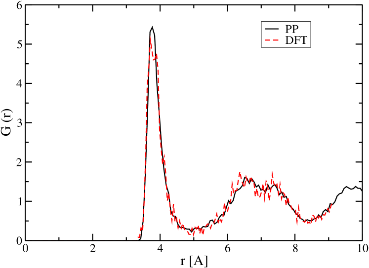
Figure 6: (Color online) Structural pair distribution function $G(r)$ for quenched structures from pair potential (solid curve, black, $N=500$) and a single DFT calculation (broken curve, red, $N=150$).

The probability of finding the system in $d\Phi_{0}$ at $\Phi_{0}$ is $P(\Phi_{0})\,\,d\Phi_{0}$, where

$$P(\Phi_{0})=\int P(\Phi_{0},\theta_{0})\,\,d\theta_{0}.$$ (8)

Upon quenching from an equilibrium trajectory at $T\geq T_{m}$, the structures sampled will exhibit a distribution of $\Phi_{0}$ proportional to $P(\Phi_{0})$. The distribution in Fig. 4 is proportional to $P(\Phi_{0})$. However, the density of states in $\Phi_{0}$ is $G(\Phi_{0})$, given by

$$G(\Phi_{0})=\int G(\Phi_{0},\theta_{0})\,\,d\theta_{0},$$ (9)

and differs from $P(\Phi_{0})$ by the statistical weight $W_{eq}(\Phi_{0},\theta_{0})$. In our studies of liquid dynamics, the purpose of quenching is to determine the densities of states $G(\Phi_{0})$ and $G(\Phi_{0},\theta_{0})$, because these are parameters of the Hamiltonian. These densities of states must be solved for from the observed distributions $P(\Phi_{0})$ and $P(\Phi_{0},\theta_{0})$ from the above equations. Even though the symmetric structures are supposed to be unimportant for the liquid as $N\rightarrow\infty$, those structures will always be statistically important at $T<T_{m}$, and will therefore be included in our analysis.

Let us introduce subscripts $r$ and $s$ for random and symmetric, respectively, and write

$$G(\Phi_{0},\theta_{0})=G_{r}(\Phi_{0},\theta_{0})+G_{s}(\Phi_{0},\theta_{0}),$$ (10)

and correspondingly $Z=Z_{r}+Z_{s}$. From Figs. 4 and 5, $P_{r}(\Phi_{0})$ at $N=500$ has very small width, comparable to experimental error in the internal energy of the liquid at melt, and this width is expected to decrease further as $N$ increases Holmström et al. (2009). These results suggest a model for $G_{r}(\Phi_{0},\theta_{0})$. Let us define the liquid $\Phi_{0}^{l}$ as the mean $\Phi_{0}$ for random structures when $N\rightarrow\infty$, with a similar definition for $\theta_{0}^{l}$. The model is

$$G_{r}(\Phi_{0},\theta_{0}) = \mathcal{N}_{r}\,\,\delta\left(\Phi_{0}-\Phi_{0}^{l}\right)\delta\left(\theta_{0}-\theta_{0}^{l}\right)\left[1+\mathcal{O}\left(N^{-\alpha}\right)\right],$$

$$G_{r}(\Phi_{0}) = \mathcal{N}_{r}\,\,\delta\left(\Phi_{0}-\Phi_{0}^{l}\right)\left[1+\mathcal{O}\left(N^{-\alpha}\right)\right],$$ (11)

where $\alpha>0$, and $\mathcal{N}_{r}$ is the number of random valleys. From this it follows that $Z_{r}=\mathcal{N}_{r}\,\,e^{-\beta\Phi_{0}^{l}}\left(T/\theta_{0}^{l}\right)^{3N}$, and the random contributions to Eqs. (7) and (8) become

$$P_{r}(\Phi_{0},\theta_{0}) = \frac{\delta\left(\Phi_{0}-\Phi_{0}^{l}\right)\delta\left(\theta_{0}-\theta_{0}^{l}\right)}{1+Z_{s}/Z_{r}}\left[1+\mathcal{O}\left(N^{-\alpha}\right)\right],$$

$$P_{r}(\Phi_{0}) = \frac{\delta\left(\Phi_{0}-\Phi_{0}^{l}\right)}{1+Z_{s}/Z_{r}}\left[1+\mathcal{O}\left(N^{-\alpha}\right)\right].$$ (12)

Hence, to finite–$N$ errors, the random valley Hamiltonian parameters $\Phi_{0}^{l}$ and $\theta_{0}^{l}$ are determined directly by quenches from equilibrium MD at $T\geq T_{m}$. And, because of the form of Eq. (11) for $G_{r}(\Phi_{0},\theta_{0})$, these observations will remain true when the statistical mechanics theory is improved to include transit effects.

The symmetric density $G_{s}(\Phi_{0},\theta_{0})$ apparently has $N$–independent width with $\Phi_{0}$ ranging from $\Phi_{0}^{bcc}$ to $\Phi_{0}^{l}$. Symmetric structures with $\Phi_{0}>\Phi_{0}^{l}$ exist, but they are rare for monatomic systems. The $\theta_{0}$ dependence of $G_{s}(\Phi_{0},\theta_{0})$ is not trivial. One expects that additional (symmetry) parameters are important for symmetric structures. Nevertheless, $G_{s}(\Phi_{0})$ and $G_{s}(\Phi_{0},\theta_{0})$ are well defined, and can be extracted from quench data with the aid of Eqs. (7) and (8).

IV.2 Quenches from stochastic configurations

On an equilibrium trajectory at $T\geq T_{m}$, the probability the system is found in a given potential energy valley is $W_{eq}(\Phi_{0},\theta_{0})$ for that valley. The statistical weight is quite different for stochastic configurations. These configurations are uniformly distributed over configuration space, except for the small excluded Cartesian–space volume at each nucleus. Neglecting this constraint, the probability the system is found in a given potential valley is the valley volume divided by the entire $3N$–dimensional volume. Let us denote the corresponding statistical weight factors as $W_{r}(\Phi_{0},\theta_{0})$ and $W_{s}(\Phi_{0},\theta_{0})$ for random and symmetric valleys respectively.

Because of their uniformity, the random valleys all have the same volume in the thermodynamic limit. To arrive at a complete solution, it is necessary to include the symmetric valleys. Let us assume that they also have a uniform configuration space volume. The number of random (symmetric) valleys is denoted $\mathcal{N}_{r}$ ($\mathcal{N}_{s}$), and the single–valley volume is $\mathcal{V}_{r}$ ($\mathcal{V}_{s}$). The statistical single–valley weights are

$$W_{r} = \frac{\mathcal{V}_{r}}{\mathcal{N}_{r}\mathcal{V}_{r}+\mathcal{N}_{s}\mathcal{V}_{s}},$$ (13)

$$W_{s} = \frac{\mathcal{V}_{s}}{\mathcal{N}_{r}\mathcal{V}_{r}+\mathcal{N}_{s}\mathcal{V}_{s}}.$$ (14)

The probability distributions are

$$P_{r}(\Phi_{0},\theta_{0}) = G_{r}(\Phi_{0},\theta_{0})W_{r},$$ (15)

$$P_{s}(\Phi_{0},\theta_{0}) = G_{s}(\Phi_{0},\theta_{0})W_{s}.$$ (16)

Hence the random and symmetric densities of states are each proportional to the distribution found in quenches from stochastic configurations. Applying the model of Eq. (11) for $G_{r}(\Phi_{0},\theta_{0})$ yields

$$P_{r}(\Phi_{0},\theta_{0})=\frac{\delta\left(\Phi_{0}-\Phi_{0}^{l}\right)\delta\left(\theta_{0}-\theta_{0}^{l}\right)}{1+\left(\mathcal{N}_{s}\mathcal{V}_{s}/\mathcal{N}_{r}\mathcal{V}_{r}\right)}\left[1+\mathcal{O}\left(N^{-\alpha}\right)\right].$$ (17)

The conclusion here is the same as with equilibrium configurations, Eq. (12), that the parameters $\Phi_{0}^{l}$ and $\theta_{0}^{l}$ are determined directly by quenches from stochastic configurations, up to finite–$N$ errors. The reason, of course, is the form of the model for $G_{r}(\Phi_{0},\theta_{0})$, Eq. (11). For symmetric structures, the above equations reveal two significant points:

1. Quenches from stochastic configurations can determine the magnitude of $G_{s}(\Phi_{0},\theta_{0})$ relative to $G_{r}(\Phi_{0},\theta_{0})$, but only when $W_{s}/W_{r}$ is known.

2. The relation between $G_{r}(\Phi_{0},\theta_{0})$ as determined by the two quench methods is unknown until $W_{s}$ is evaluated.

These points are relevant to the distributions shown in Figs. 4 and 5.

V Conclusions

In this article, we have addressed two main research goals: (1) The use of stochastic configurations to probe the distribution of potential energy minima, and (2) the calibration of the V-T Hamiltonian with DFT.

V.1 Stochastic Configurations

Quenches from stochastic configurations produce statistically indistinguishable distributions of the potential energy, $\Phi_{0}/N$, compared to quenches from equilibrium liquid MD trajectories. We have demonstrated that quenching from stochastic configurations can be used to find the entire distribution of Na potential energy minima, i.e. they reliably reproduce the correct distribution of random and symmetric structures. This is illustrated by a comparison of $\Phi_{0}/N$ distributions for quenches from equilibrium MD and from stochastic configurations (Figs. 4 and 5, Sec. III.1). Quenches from stochastic configurations yield an accurate random distribution for Na in agreement with the random distribution from quenches from equilibrium MD, Eq. (1).

Compared to generating and selecting configurations from equilibrium MD trajectories, our stochastic configuration method is significantly faster and more economical (Sec. II). Stochastic configurations do not require interatomic potentials or costly equilibration and long simulation times. Simply generate random Cartesian coordinates for each atom under a minimal excluded–volume constraint to eliminate particle overlap. Hence, this procedure requires very little computational effort, an economy that accommodates ab initio quench methods even for large systems.

V.2 Calibration of the V-T Hamiltonian

Calibration of the V-T Hamiltonian is based on the presumed dominance and uniformity of random valleys as $N\rightarrow\infty$. This view is given mathematical expression in the model for $G_{r}(\Phi_{0},\theta_{0})$, Eq. (11). It follows that the thermodynamic limit parameters $\Phi_{0}^{l}$ and $\theta_{0}^{l}$ are determined directly from data for either MD quenches or stochastic quenches, up to finite–$N$ errors.

We have demonstrated that the DFT structure in Sec. III.2 is random by comparing the mean potential energy $\Phi_{0}/N$ with the pair potential results in Eq. (3), the phonon moment $\theta_{0}$ in Eq. (4), and the pair distribution function $G(r)$ in Fig. 6. We conclude that being random, the DFT structure can provide ab initio calibration of the V-T Hamiltonian.

As verified by their pair distribution function, stochastic configurations have nuclei distributed nearly uniformly over the system volume (Figs. 1 and 2, Sec. II). Therefore among stochastic configurations, the statistical weight for a many–atom potential energy valley is (nearly) proportional to the valley volume. This is in contrast to quenches from equilibrium MD, which require extensive modeling to extract the Boltzmann factor from the weight Heuer and Büchner (2000). Given the statistical weight, characteristics of the underlying potential surface can be extracted from data acquired by stochastic quenches (Sec. IV).

We do not suggest that DFT quenches from stochastic configurations will invariably arrive at random structures, just as quenches from an equilibrium MD trajectory may result in a symmetric structure. Indeed, some symmetric structures have appeared in our DFT quenches. Precisely what is required to eliminate symmetric structures from any collection of quench data is an ongoing research question.

VI Acknowledgments

EH and RL would like to thank Fondecyt projects 11070115 and 11080259. They are also thankful for the support of “Proyecto Anillo” ACT-24. This work was funded by the US Department of Energy under contract number DE-AC52-06NA25396. The open and friendly scientific atmosphere of the Ten Bar International Science Café is also acknowledged.

References

- Wallace (1997) D. C. Wallace, Phys. Rev. E 56, 4179 (1997).
- Chisolm and Wallace (2001) E. D. Chisolm and D. C. Wallace, J. Phys.: Condens. Matter 13, R739 (2001).
- De Lorenzi-Venneri and Wallace (2007) G. De Lorenzi-Venneri and D. C. Wallace, Phys. Rev. E 76, 041203 (2007).
- Car and Parrinello (1985) R. Car and M. Parrinello, Phys. Rev. Lett. 55, 2471 (1985).
- Sugino and Car (1995) O. Sugino and R. Car, Phys. Rev. Lett. 74, 1823 (1995).
- Kresse and Hafner (1993a) G. Kresse and J. Hafner, Phys. Rev. B 47, 558 (1993a).
- Kresse and Hafner (1993b) G. Kresse and J. Hafner, Phys. Rev. B 48, 13115 (1993b).
- Kresse (2002) G. Kresse, J. Non-Cryst. Solids 312–314, 52 (2002).
- de Wijs et al. (1998) G. A. de Wijs, G. Kresse, and M. J. Gillan, Phys. Rev. B 57, 8223 (1998).
- Alfè et al. (2000) D. Alfè, G. Kresse, and M. J. Gillan, Phys. Rev. B 61, 132 (2000).
- Chai et al. (2003) J.-D. Chai, D. Stroud, J. Hafner, and G. Kresse, Phys. Rev. B 67, 104205 (2003).
- Kresse and Furthmüller (1996) G. Kresse and J. Furthmüller, Computational Materials Science 6, 15 (1996).
- Stillinger and Weber (1982) F. H. Stillinger and T. A. Weber, Phys. Rev. A 25, 978 (1982).
- Weber and Stillinger (1984) T. A. Weber and F. H. Stillinger, J. Chem. Phys. 80, 2742 (1984).
- Stillinger and Weber (1984) F. H. Stillinger and T. A. Weber, Science 225, 983 (1984).
- Heuer and Büchner (2000) A. Heuer and S. Büchner, J. Phys.: Condens. Matter 12, 6535 (2000).
- Sciortino et al. (1999) F. Sciortino, W. Kob, and P. Tartaglia, Phys. Rev. Lett. 83, 3214 (1999).
- Holmström et al. (2009) E. Holmström, N. Bock, T. B. Peery, R. Lizárraga, G. De Lorenzi-Venneri, E. D. Chisolm, and D. C. Wallace (2009), work in progress.
- Wallace (1968) D. C. Wallace, Phys. Rev. 176, 832 (1968).
- Wallace (2002) D. C. Wallace, Statistical Physics of Crystals and Liquids (World Scientific, New Jersey, 2002).
- Bock et al. (2008) N. Bock, T. Peery, E. D. Chisolm, G. De Lorenzi-Venneri, D. C. Wallace, E. Holmström, and R. Lizárraga, Bull. Am. Phys. Soc. 53 (2), J9:00004 (2008).
- Chakravarty et al. (2005) C. Chakravarty, P. G. Debenedetti, and F. H. Stillinger, J. Chem. Phys. 123, 206101 (2005).
- Chakraborty and Chakravarty (2006) S. N. Chakraborty and C. Chakravarty, J. Chem. Phys. 124, 014507 (2006).
- Wallace and Clements (1999) D. C. Wallace and B. E. Clements, Phys. Rev. E 59, 2942 (1999).
- Clements and Wallace (1999) B. E. Clements and D. C. Wallace, Phys. Rev. E 59, 2955 (1999).
- (26) Vienna Ab-initio Simulation Package (VASP), URL http://cms.mpi.univie.ac.at/vasp/.
- Blöchl (1994) P. E. Blöchl, Phys. Rev. B 50, 17953 (1994).
- Kresse and Joubert (1999) G. Kresse and D. Joubert, Phys. Rev. B 59, 1758 (1999).
- Monkhorst and Pack (1976) H. J. Monkhorst and J. D. Pack, Phys. Rev. B 13, 5188 (1976).
- (30) An equilibrium MD system moves at constant total energy and total momentum. These constraints affect fluctuations in order 1, but affect mean values only in order Lebowitz et al. (1967). We exercise caution when using canonical weighting to analyze MD results.
- Lebowitz et al. (1967) J. L. Lebowitz, J. K. Percus, and L. Verlet, Phys. Rev. 153, 250 (1967).