Approximate expression for the dynamic structure factor in the Lieb-Liniger model

Abstract

Recently, Imambekov and Glazman [Phys. Rev. Lett. 100, 206805 (2008)] showed that the dynamic structure factor (DSF) of the 1D Bose gas demonstrates power-law behaviour along the limiting dispersion curve of the collective modes and calculated the corresponding exponents exactly. Combining these recent results with a previously obtained strong-coupling expansion we present an interpolation formula for the DSF of the 1D Bose gas. The obtained expression is further consistent with exact low energy exponents from Luttinger liquid theory and shows nice agreement with recent numerical results.

cherny@theor.jinr.ru

Cigar-shaped traps with cold alkali atoms have recently been used to obtain a quasi-1D quantum degenerate Bose gas, where atomic motion in the transverse dimensions is confined to zero-point quantum oscillations, in weak and strong interaction regimes [1, 2]. Theoretically, we may describe the system as a one-dimensional rarefied gas where interactions of bosonic atoms can be described well by effective $\delta$-function interactions [3]. Thus the Lieb-Liniger model [4, 5] is applicable. Being exactly solvable in the uniform case, the model, however, does not admit complete analytic solutions for the correlation functions. Up to now, this has been an outstanding problem in 1D physics [6, 7]. Here, we propose an approximate formula for the DSF of the Lieb-Liniger gas that is consistent with known results in accessible limits and power laws.

Dynamical density-density correlations, which can be measured by the two-photon Bragg scattering [8, 9], are described by the dynamic structure factor (DSF) [10]

$$S(q,\omega)=L\int\frac{\mathrm{d}t\mathrm{d}x}{2\pi\hbar}\,e^{i(\omega t-qx)}\langle 0|\delta\hat{\rho}(x,t)\delta\hat{\rho}(0,0)|0\rangle.$$ (1)

Here, we introduce the density fluctuations $\delta\hat{\rho}(x,t)\equiv\hat{\rho}(x,t)-n$ and the equilibrium density of particles $n=N/L$. We consider the case of zero temperature, where $\langle 0|\ldots|0\rangle$ means ground-state average. The DSF is proportional to the probability of exciting the collective mode from the ground state with momentum $q$ and energy $\hbar\omega$ transfer, as one can see in the energy representation of Eq. (1)

$$S(k,\omega)=\sum_{n}|\langle 0|\delta\hat{\rho}_{k}|n\rangle|^{2}\delta(\hbar\omega-E_{n}+E_{0}),$$ (2)

where $\delta\hat{\rho}_{k}=\sum_{j}e^{-ikx_{j}}$ is the Fourier component of $\delta\hat{\rho}(x)$.

The Lieb-Liniger model [4, 5] represents a uniform 1D system of spinless bosons of mass $m$, interacting with pairwise point interactions $V(x)=g_{\rm B}\delta(x)$; the interaction strength $g_{\rm B}$ is assumed to be positive. Periodic boundary conditions are imposed on the wave functions. The strength of interactions can be measured in terms of the dimensionless Lieb-Liniger parameter $\gamma\equiv mg_{\mathrm{B}}/(\hbar^{2}n)$. Within the Lieb-Liniger model, the DSF has the following well-established properties.

i) Luttinger liquid theory predicts a power-law behaviour of the DSF at low energies in the vicinity of the momenta $k=0,2\pi n,4\pi n\ldots$ and yields model-independent values of the exponents [11, 12]. In particular, one can show [12, 13] that in the vicinity of “umklapp” point ($k=2\pi n$, $\omega=0$)

$$S(k,\omega)\sim(\omega^{2}-\omega^{2}_{-})^{K-1},$$ (3)

where $K\equiv\hbar\pi n/(mc)$ and $c$ is sound velocity. Furthermore, within the Luttinger-liquid theory, the dispersion is linear in vicinity of the umklapp point: $\omega_{-}(k)\simeq c|k-2\pi n|$. Relation (3) leads to different exponents precisely at the umklapp point and outside of it:

$$S(k,\omega)\sim\left\{\begin{array}[]{ll}\omega^{2(K-1)},&k=2\pi n,\\ (\omega-\omega_{-})^{K-1},&k\not=2\pi n.\end{array}\right.$$ (4)

ii) By using in a non-trivial manner the Bose-Fermi mapping in 1D [14], the authors developed the time-dependent Hartree-Fock scheme [15, 16] in the strong-coupling regime with the small parameter $1/\gamma$. The scheme guarantees validity of the DSF expansion [15, 16]

$$S(k,\omega)\frac{\varepsilon_{\mathrm{F}}}{N}=\frac{k_{\mathrm{F}}}{4k}\left(1+\frac{8}{\gamma}\right)+\frac{1}{2\gamma}\ln\frac{\omega^{2}-\omega_{-}^{2}}{\omega_{+}^{2}-\omega^{2}}+O\left(\frac{1}{\gamma^{2}}\right),$$ (5)

for $\omega_{-}\leq\omega\leq\omega_{+}$, and zero otherwise. Here $\omega_{\pm}(k)$ are the limiting dispersions that bounds quasiparticle-quasihole excitations [5]. In the strong-coupling regime they take the form $\omega_{\pm}(k)={\hbar|2k_{\mathrm{F}}k\pm k^{2}|}(1-4/\gamma)/{(2m)}+O\left(\gamma^{-2}\right)$. By definition, $k_{\mathrm{F}}\equiv\pi n$ and $\varepsilon_{\mathrm{F}}\equiv\hbar^{2}k_{\mathrm{F}}^{2}/(2m)$ are the Fermi wave vector and energy of a non-interacting Fermi gas, respectively.

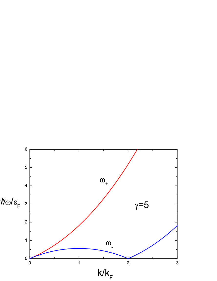
Figure 1: Limiting dispersions $\omega_{\pm}$ versus wave vector $k$ for the coupling parameter $\gamma=5$. The data are obtained numerically by solving Lieb-Liniger’s system of integral equations [5, 6].

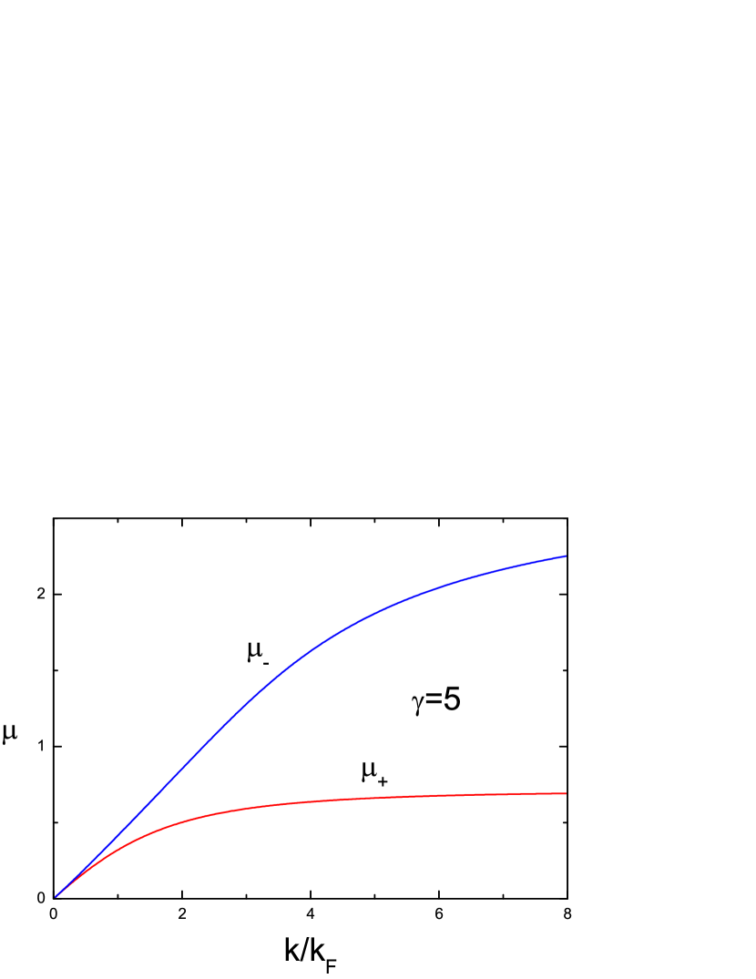
Figure 2: Typical behaviour of the exact exponents in Eq. (6). The plot shows $\mu_{\pm}$ for $\gamma=5$ obtained numerically using the method of Ref. [17].

iii) As was shown by Imambekov and Glazman [17], in the Lieb-Liniger model the DSF demonstrates power-law behaviour near the borders $\omega_{\pm}(k)$

$$S(k,\omega)\sim\big{|}\omega-\omega_{\pm}(k)\big{|}^{\mp\mu_{\pm}(k)}.$$ (6)

The positive exponents $\mu_{\pm}$ [18] are related to the quasi-particle scattering phase and can be easily evaluated by solving a system of a few integral equations in thermodynamic limit [17]. We obtain the exact relation

$$\mu_{-}(2\pi n-0)=2\sqrt{K}(\sqrt{K}-1),$$ (7)

which obviously differs from the Luttinger liquid exponent (4) for $k\not=2\pi n$. However, Imambekov’s and Glazman’s result (7) is correct in the immediate vicinity of $\omega_{\pm}$ provided that the finite curvature of $\omega_{-}(k)$ is taken into consideration. Thus the difference in the exponents can be treated [17] as an artifact of the linear spectrum approximation in the Luttinger liquid theory. Note, however, that the thin “strip” in $\omega$-$k$ plane where the exponents are different vanishes in the point $k=2\pi n$; hence, the Luttinger exponent $2(K-1)$ should be exact here.

iv) The DSF can be calculated numerically by means of algebraic Bethe ansatz [19].

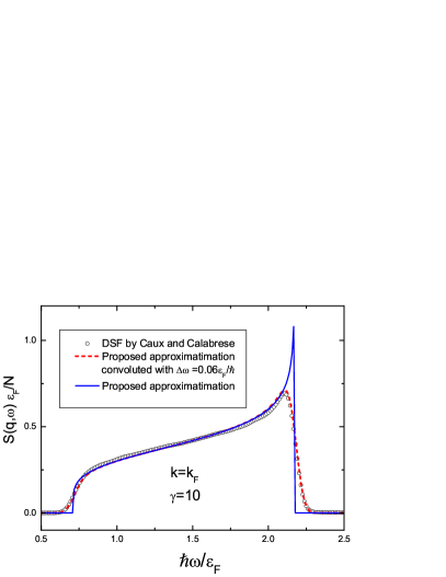
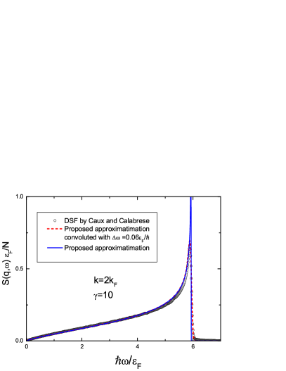
Figure 3: The Dynamic Structure Factor (DSF) in the thermodynamic limit. The proposed approximation (8) (line) is compared to numerical data from Caux and Calabrese [19] (open dots). The dashed (red) line shows the data of Eq. (8) convoluted in frequency with a Gaussian of width $\Delta\omega\sqrt{2\ln 2}=0.07\varepsilon_{\mathrm{F}}/\hbar$ in order to simulate smearing that has been used in generating the numerical results of Ref. [19]. The numerical data of Ref. [19] suggests that contributions from multi-particle excitations for $\omega>\omega_{+}$ (sharp line in parts a and b) are very small. Such contributions are not accounted for by the formula (8).

Here we suggest a phenomenological expression, which is consistent with all of the above-mentioned results. It reads

$$S(k,\omega)=C\frac{(\omega^{\alpha}-\omega_{-}^{\alpha})^{\mu_{-}}}{(\omega_{+}^{\alpha}-\omega^{\alpha})^{\mu_{+}}}$$ (8)

for $\omega_{-}(k)\leq\omega\leq\omega_{+}(k)$, and zero otherwise. Here $C$ is a normalization constant, $\mu_{+}(k)$ and $\mu_{-}(k)$ are the exponents of Eq. (6), and $\alpha\equiv 1+1/\sqrt{K}$. The normalization constant depends on momentum but not frequency and can be determined from the $f$-sum rule (see, e.g., Ref. [10])

$$\int_{-\infty}^{+\infty}\mathrm{d}\omega\,\omega S(q,\omega)=N\frac{q^{2}}{2m}.$$ (9)

We assume that in Eq. (8) the value of the exponent $\mu_{-}(k=2\pi n)$ coincides with its limiting value (7) in vicinity of the umklapp point.

Now it can be easily seen from (8) that

$$S(k,\omega)\sim\left\{\begin{array}[]{ll}\omega^{2(K-1)},&k=2\pi n,\\ (\omega-\omega_{-})^{\mu_{-}(k)},&k\not=2\pi n.\end{array}\right.$$ (10)

Thus, the suggested formula is consistent with the both the Luttinger liquid behaviour at the umklapp point and Imambekov’s and Glazman’s power-law behaviour in vicinity of it, as it should be.

In the strong-coupling regime, Eq. (8) correctly yields the first order expansion (5). In order to prove this, it is sufficient to use the strong-coupling values of $K=1+4/\gamma+O(1/\gamma^{2})$, $\mu_{\pm}(k)=2\arctan[k/(n\gamma)]/\pi+O(1/\gamma^{2})$ (see Ref. [20]), and the frequency dispersions.

Comparison with numerical data by Caux and Calabrese [19] (figure 3) shows that the suggested formula nicely works in the regimes of both weak and strong coupling.

Concluding, we propose the approximate formula (8) for DSF of the one-dimensional Bose gas at zero temperature. It neglects, in effect, only the contributions of multiparticle excitations outside the bounds given by the dispersion curves $\omega_{\pm}$, whose contribution is small. Our formula is consistent with predictions of Luttinger liquid theory, has the exact exponents at the edge of the spectrum, gives the correct first-order expansion in the strong-coupling regime, and shows nice agreement with available numerical data.

The authors are grateful to Jean-Sebastien Caux for making the data of numerical calculations of Ref. [19] available to us and to Thomas Ernst for checking our numerical results. This project received funding from the Marsden fund of New Zealand under contract number MAU0607. AYuCh thanks Massey University for hospitality.

References

References

- [1] Görlitz A, Vogels J M, Leanhardt A E, Raman C, Gustavson T L, Abo-Shaeer J R, Chikkatur A P, Gupta S, Inouye S, Rosenband T and Ketterle W 2001 Phys. Rev. Lett. 87 130402
- [2] Kinoshita T, Wenger T and Weiss D S 2004 Science 305 1125–1128
- [3] Olshanii M 1998 Phys. Rev. Lett. 81 938–941
- [4] Lieb E H and Liniger W 1963 Phys. Rev. 130 1605–1616
- [5] Lieb E H 1963 Phys. Rev. 130 1616–1624
- [6] Korepin V E, Bogoliubov N M and Izergin A G 1993 Quantum Inverse Scattering Method and Correlation Functions (Cambridge: University)
- [7] Giamarchi T 2004 Quantum Physics in One Dimension (Oxford: Clarendon)
- [8] Stenger J, Inouye S, Chikkatur A P, Stamper-Kurn D M, Pritchard D E and Ketterle W 1999 Phys. Rev. Lett. 82 4569–4573
- [9] Ozeri R, Katz N, Steinhauer J and Davidson N 2005 Rev. Mod. Phys. 77 187
- [10] Pitaevskii L and Stringari S 2003 Bose-Einstein Condensation (Oxford: Clarendon)
- [11] Haldane F D M 1981 Phys. Rev. Lett. 47 1840
- [12] Astrakharchik G E and Pitaevskii L P 2004 Phys. Rev. A 70 013608
- [13] A H Castro Neto, Lin H Q, Chen Y H and Carmelo J M P 1994 Phys. Rev. B 50 14032
- [14] Cheon T and Shigehara T 1999 Phys. Rev. Lett. 82 2536
- [15] Brand J and Cherny A Y 2005 Phys. Rev. A 72 033619
- [16] Cherny A Y and Brand J 2006 Phys. Rev. A 73 023612
- [17] Imambekov A and Glazman L I 2008 Phys. Rev. Lett. 100 206805
- [18] We slightly change the notations: ours and correspond to and , respectively, in Ref. [17].
- [19] Caux J S and Calabrese P 2006 Phys. Rev. A 74 031605
- [20] Khodas M, Pustilnik M, Kamenev A and Glazman L I 2007 Phys. Rev. Lett. 99 110405