A New Approach To The Treatment Of Separatrix Chaos And Its Applications

Abstract

We consider time-periodically perturbed 1D Hamiltonian systems possessing one or more separatrices. If the perturbation is weak, then the separatrix chaos is most developed when the perturbation frequency lies in the logarithmically small or moderate ranges: this corresponds to the involvement of resonance dynamics into the separatrix chaos. We develop a method matching the discrete chaotic dynamics of the separatrix map and the continuous regular dynamics of the resonance Hamiltonian. The method has allowed us to solve the long-standing problem of an accurate description of the maximum of the separatrix chaotic layer width as a function of the perturbation frequency. It has also allowed us to predict and describe new phenomena including, in particular: (i) a drastic facilitation of the onset of global chaos between neighbouring separatrices, and (ii) a huge increase in the size of the low-dimensional stochastic web.

1 Introduction

Separatrix chaos is the germ of Hamiltonian chaos zaslavsky:1998 . Consider an integrable Hamiltonian system possessing a saddle, i.e. a hyperbolic point in the one-dimensional case, or a hyperbolic invariant torus, in higher-dimensional cases. The stable (incoming) and unstable (outgoing) manifolds of the saddle are called separatrices gelfreich : they separate trajectories that have different phase space topologies. If a weak time-periodic perturbation is added, then the separatrix is destroyed; it is replaced by a separatrix chaotic layer (SCL) zaslavsky:1998 ; gelfreich ; lichtenberg_lieberman ; treschev . Even if the unperturbed system does not possess a separatrix, the resonant part of the perturbation generates a separatrix in the auxiliary resonance phase space while the non-resonant part of the perturbation destroys this separatrix, replacing it with a chaotic layer zaslavsky:1998 ; gelfreich ; lichtenberg_lieberman ; Chirikov:79 . Thus separatrix chaos is of a fundamental importance for Hamiltonian chaos.

One of the most important characteristics of SCL is its width in energy (or expressed in related quantities). It can be easily found numerically by integration of the Hamiltonian equations with a set of initial conditions in the vicinity of the separatrix: the space occupied by the chaotic trajectory in the Poincaré section has a higher dimension than that for a regular trajectory, e.g. in the 3/2D case the regular trajectories lie on lines i.e. 1D objects while the chaotic trajectory lies within the SCL i.e. the object outer boundaries of which limit a 2D area.

On the other hand, it is important to be able to describe theoretically both the outer boundaries of the SCL and its width. There is a long and rich history of the such studies. The results may be classified as follows.

1.1 Heuristic results

Consider a 1D Hamiltonian system perturbed by a weak time-periodic perturbation:

$$H=H_{0}(p,q)+hV(p,q,t),$$ (1)

$$V(p,q,t+2\pi/\omega_{f})=V(p,q,t),\quad\quad h\ll 1,$$

where $H_{0}(p,q)$ possesses a separatrix and, for the sake of notational compactness, all relevant parameters of $H_{0}$ and $V$, except possibly for $\omega_{f}$, are assumed to be $\sim 1$.

Physicists proposed a number of different heuristic criteria ZF:1968 ; Chirikov:79 ; lichtenberg_lieberman ; Zaslavsky:1991 ; zaslavsky:1998 ; zaslavsky:2005 for the SCL width $\Delta E$ in terms of energy $E\equiv H_{0}(p,q)$ which gave qualitatively similar results:

$$\Delta E\equiv\Delta E(\omega_{f})\sim\omega_{f}\delta,\quad\quad$$ (2)

$$\delta\equiv h|\epsilon|,$$

$$|\epsilon|\stackrel{{\scriptstyle<}}{{\sim}}1\quad\quad\quad\quad\quad\quad\quad\quad\quad\quad\quad\quad\quad{\rm for}\quad\omega_{f}\stackrel{{\scriptstyle<}}{{\sim}}1,$$

$$|\epsilon|\propto\exp(-a\omega_{f})\ll 1\quad\quad(a\sim 1)\quad\quad{\rm for}\quad\omega_{f}\gg 1.$$

The quantity $\delta\equiv h|\epsilon|$ is called the separatrix split zaslavsky:1998 (see also Eq. (4) below): it determines the maximum distance between the perturbed incoming and outgoing separatrices ZF:1968 ; Chirikov:79 ; lichtenberg_lieberman ; Zaslavsky:1991 ; zaslavsky:1998 ; zaslavsky:2005 ; abdullaev ; gelfreich ; treschev .

It follows from (2) that the maximum of $\Delta E$ should lie in the frequency range $\omega_{f}\sim 1$ while the maximum itself should be $\sim h$:

$$\Delta E_{\max}\equiv\max_{\omega_{f}}\{\Delta E(\omega_{f})\}\sim h,\quad\quad\quad\omega_{f}^{(\max)}\sim 1.$$ (3)

1.2 Mathematical and accurate physical results

Many papers studied the SCL by mathematical or accurate physical methods.

For the range $\omega_{f}\gg 1$, many works studied the separatrix splitting (see the review gelfreich and references therein) and the SCL width in terms of normal coordinates (see the review treschev and references therein). Though quantities studied in these works differ from those typically studied by physicists ZF:1968 ; Chirikov:79 ; lichtenberg_lieberman ; Zaslavsky:1991 ; zaslavsky:1998 ; zaslavsky:2005 , they implicitly confirm the main qualitative conclusion from the heuristic formula (2) in the high frequency range: provided that $\omega_{f}\gg 1$ the SCL width is exponentially small.

There were also several works studying the SCL in the opposite (i.e. adiabatic) limit $\omega_{f}\rightarrow 0$: see e.g. Neishtadt:1986 ; E&E:1991 ; Neishtadt:1997 ; prl2005 ; 13_prime and references therein. In the context of the SCL width, it is most important that $\Delta E(\omega_{f}\rightarrow 0)\sim h$ for most of the systems Neishtadt:1986 ; E&E:1991 ; Neishtadt:1997 . For a particular class of systems, namely for ac-driven spatially periodic systems (e.g. the ac-driven pendulum), the width of the SCL part above the separatrix diverges in the adiabatic limit prl2005 ; 13_prime : the divergence develops for $\omega_{f}\ll 1/\ln(1/h)$.

Finally, there is a qualitative estimation of the SCL width for the range $\omega_{f}\sim 1$ within the Kolmogorov-Arnold-Moser (KAM) theory treschev . The quantitative estimate within the KAM theory is lacking, apparently being very difficult for this frequency range vasya . It follows from the results in treschev that the width in this range is of the order of the separatrix split, which itself is of the order of $h$.

Thus it could seem to follow that, for all systems except ac-driven spatially periodic systems, the maximum in the SCL width is $\sim h$ and occurs in the range $\omega_{f}\sim 1$, very much in agreement with the heuristic result (3). Even for ac-driven spatially periodic systems, this conclusion could seem to apply to the width of the SCL part below the separatrix over the whole frequency range, and to the width of the SCL part above the separatrix for $\omega_{f}\stackrel{{\scriptstyle>}}{{\sim}}1/\ln(1/h)$.

1.3 Numerical evidence for high peaks in $\Delta E(\omega_{f})$ and their rough estimation

The above conclusion disagrees with several numerical studies carried out during the last decade (see e.g. prl2005 ; 13_prime ; shevchenko:1998 ; luo1 ; soskin2000 ; luo2 ; vecheslavov ; shevchenko ) which have revealed the existence of sharp peaks in $\Delta E(\omega_{f})$ in the frequency range $1/\ln(1/h)\stackrel{{\scriptstyle<}}{{\sim}}\omega_{f}\stackrel{{\scriptstyle<}}{{\sim}}1$ the heights of which greatly exceed $h$ (see also Figs. 2, 3, 5, 6 below). Thus, the peaks represent the general dominant feature of the function $\Delta E(\omega_{f})$. They were related by the authors of shevchenko:1998 ; luo1 ; soskin2000 ; luo2 ; vecheslavov ; shevchenko to the absorption of nonlinear resonances by the SCL. For some partial case, rough heuristic estimates for the position and magnitude of the peaks were made in shevchenko:1998 ; shevchenko .

1.4 Accurate description of the peaks and of the related phenomena

Until recently, accurate analytic estimates for the peaks were lacking. It is explicitly stated in luo2 that the search for the mechanism through which resonances are involved in separatrix chaos, and for an accurate analytic description of the peaks in the SCL width as function of the perturbation frequency, are being among the most important and challenging tasks in the study of separatrix chaos. The first step towards accomplishing them was taken through the proposal pre2008 ; proceedings of a new approach to the theoretical treatment of the separatrix chaos in the relevant frequency range. It was developed and applied to the onset of global chaos between two close separatrices. The application of the approach pre2008 ; proceedings to the commoner single-separatrix case was also discussed. The approach has been further developed icnf_approach ; pre_submitted , including an explicit theory for the single-separatrix case pre_submitted .

The present paper reviews the new approach pre2008 ; proceedings ; icnf_approach ; pre_submitted and its applications to the single-separatrix pre_submitted and double-separatrix pre2008 ; proceedings cases. We also briefly review application to the enlargement of the low-dimensional stochastic web icnf_enlargement and discuss other promising applications.

Though the form of our treatment differs from typical forms of mathematical theorems in this subject (cf. gelfreich ; treschev ), it yields the exact expressions for the leading term in the relevant asymptotic expansions (the parameter of smallness is $\alpha\equiv 1/\ln(1/h)$) and, in some case, even for the next-order term. Our theory is in excellent agreement with results obtained by numerical integration of the equations of motion.

Sec. 2 describes the basic ideas underlying the approach. Sec. 3 is devoted to the leading-order asymptotic description of the single-separatrix chaotic layers. Sec. 4 presents an asymptotic description of the onset of global chaos in between two close separatrices. Sec. 5 describes the increase in sizes of a stochastic web. Conclusions are drawn in Sec. 6. Sec. 7 presents the Appendix, which explicitly matches the separatrix map and the resonance Hamiltonian descriptions for the double-separatrix case.

2 Basic ideas of the approach

The new approach pre2008 ; proceedings ; icnf_approach ; pre_submitted may be formulated briefly as a matching between the discrete chaotic dynamics of the separatrix map in the immediate vicinity of the separatrix and the continuous regular dynamics of the resonance Hamiltonian beyond that region. The present section describes the general features of the approach in more detail.

Motion near the separatrix may be approximated by the separatrix map (SM) ZF:1968 ; Chirikov:79 ; lichtenberg_lieberman ; Zaslavsky:1991 ; zaslavsky:1998 ; zaslavsky:2005 ; abdullaev ; treschev ; shevchenko:1998 ; shevchenko ; pre2008 ; proceedings ; vered . This was introduced in ZF:1968 and its various modifications were subsequently used in many studies. It is sometimes known as the whisker map. It was re-derived rigorously in vered as the leading-order approximation of motion near the separatrix in the asymptotic limit $h\rightarrow 0$, and an estimate of the error was also carried out in vered (see also the review treschev and references therein).

The main ideas that allow one to introduce the SM ZF:1968 ; Chirikov:79 ; lichtenberg_lieberman ; Zaslavsky:1991 ; zaslavsky:1998 ; zaslavsky:2005 ; abdullaev ; treschev ; pre2008 ; proceedings ; vered are as follows. For the sake of simplicity, let us consider a perturbation $V$ that does not depend on the momentum: $V\equiv V(q,t)$. A system with energy close to the separatrix value spends most of its time in the vicinity of the saddle(s), where the velocity $\dot{q}$ is exponentially small. Differentiating $E\equiv H_{0}(p,q)$ with respect to time and allowing for the equations of motion of the system (1), we can show that ${\rm d}E/{\rm d}t\equiv\partial V/\partial q\dot{q}\propto\dot{q}$. Thus, the perturbation can significantly change the energy only when the velocity is not small i.e. during the relatively short intervals while the system is away from the saddle(s): these intervals correspond to pulses of velocity as a function of time (cf. Fig. 20 in the Appendix below). Consequently, it is possible to approximate the continuous Hamiltonian dynamics by a discrete dynamics which maps the energy $E$, the perturbation angle $\varphi\equiv\omega_{f}t$, and the velocity sign $\sigma\equiv{\rm sgn}(\dot{q})$, from pulse to pulse.

The actual form of the SM may vary, depending on the system under study, but its features relevant in the present context are similar for all systems. For the sake of clarity, consider the explicit case when the separatrix of $H_{0}(p,q)$ possesses a single saddle and two symmetric loops while $V=q\cos(\omega_{f}t)$. Then the SM reads pre2008 (cf. Appendix):

$$E_{i+1}=E_{i}+\sigma_{i}h\epsilon\sin(\varphi_{i}),$$ (4)

$$\varphi_{i+1}=\varphi_{i}+\frac{\omega_{f}\pi(3-{\rm sgn}(E_{i+1}-E_{s}))}{2\omega(E_{i+1})},$$

$$\sigma_{i+1}=\sigma_{i}\,{\rm sgn}(E_{s}-E_{i+1}),\quad\quad|\sigma_{i}|=1,$$

$$\quad\quad\quad\epsilon\equiv\epsilon(\omega_{f})={\rm sgn}\left(\left.\frac{\partial H_{0}}{\partial p}\right|_{t\rightarrow-\infty}\right)\int_{-\infty}^{\infty}{\rm d}t\;\left.\frac{\partial H_{0}}{\partial p}\right|_{E_{s}}\sin(\omega_{f}t),$$

$$\quad\quad\quad E_{i}\equiv\left.H_{0}(p,q)\right|_{t_{i}-\Delta},\quad\quad\varphi_{i}\equiv\omega_{f}t_{i},\quad\quad\sigma_{i}\equiv{\rm sgn}\left(\left.\frac{\partial H_{0}}{\partial p}\right|_{t_{i}}\right),$$

where $E_{s}$ is the separatrix energy, $\omega(E)$ is the frequency of oscillation with energy $E$ in the unperturbed case (i.e. for $h=0$), $t_{i}$ is the instant corresponding to the $i$-th turning point in the trajectory $q(t)$ (cf. Fig. 20 in the Appendix below), and $\Delta$ is an arbitrary value from the range of time intervals which greatly exceed the characteristic duration of the velocity pulse while being much smaller than the interval between the subsequent pulses ZF:1968 ; Chirikov:79 ; lichtenberg_lieberman ; Zaslavsky:1991 ; zaslavsky:1998 ; zaslavsky:2005 ; abdullaev ; treschev ; vered . Consider the two most general ideas of our approach.

1. If a trajectory of the SM includes a state with $E=E_{s}$ and an arbitrary $\varphi$ and $\sigma$, then this trajectory is chaotic. Indeed, the angle $\varphi$ of such a state is not correlated with the angle of the state at the previous step of the SM, due to the divergence of $\omega^{-1}(E\rightarrow E_{s})$. Therefore, the angle at the previous step may deviate from a multiple of $2\pi$ by an arbitrary value. Hence the energy of the state at the previous step may deviate from $E_{s}$ by an arbitrary value within the interval $[-h|\epsilon|,h|\epsilon|]$. The velocity sign $\sigma$ is not correlated with that at the previous step either. Given that a regular trajectory of the SM cannot include a step where all three variables change random-like, we conclude that such a trajectory must be chaotic.

   Though the above arguments may appear to be obvious, they cannot be considered a mathematically rigorous proof, so that the statement about the chaotic nature of the SM trajectory which includes any state with $E=E_{s}$ should be considered as a conjecture supported by the above arguments and by numerical iteration of the SM. Possibly, a mathematically rigorous proof should involve an analysis of the Lyapunov exponents for the SM (cf. lichtenberg_lieberman ) but this appears to be a technically difficult problem. We emphasize however that a rigorous proof of the conjecture is not crucial for the validity of the main results of the present paper, namely for the leading terms in the asymptotic expressions describing (i) the peaks of the SCL width as a function of the perturbation frequency in the single-separatrix case, and (ii) the related quantities for the double-separatrix case. It will become obvious from the next item that, to derive the leading term, it is sufficient to know that the chaotic trajectory does visit areas of the phase space where the energy deviates from the separatrix by values of the order of the separatrix split $\delta\equiv h|\epsilon|$, which is a widely accepted fact ZF:1968 ; Chirikov:79 ; lichtenberg_lieberman ; Zaslavsky:1991 ; zaslavsky:1998 ; zaslavsky:2005 ; abdullaev ; gelfreich ; treschev .

2. It is well known ZF:1968 ; Chirikov:79 ; lichtenberg_lieberman ; Zaslavsky:1991 ; zaslavsky:1998 ; zaslavsky:2005 ; abdullaev ; gelfreich ; treschev ; shevchenko:1998 ; shevchenko ; pre2008 ; proceedings , that, at the leading-order approximation, the frequency of eigenoscillation as function of the energy near the separatrix is proportional to the reciprocal of the logarithmic factor

   $$\omega(E)=\frac{b\pi\omega_{0}}{\ln\left(\frac{\Delta H}{|E-E_{s}|}\right)},\quad b=\frac{3-{\rm sgn}(E-E_{s})}{2},$$ (5)

   $$|E-E_{s}|\ll\Delta H\equiv E_{s}-E_{st},$$

   where $E_{st}$ is the energy of the stable states.

   Given that the argument of the logarithm is large in the relevant range of $E$, the function $\omega(E)$ is nearly constant for a substantial variation of the argument. Therefore, as the SM maps the state $(E_{0}=E_{s},\varphi_{0},\sigma_{0})$ onto the state with $E=E_{1}\equiv E_{s}+\sigma_{0}h\epsilon\sin(\varphi_{0})$, the value of $\omega(E)$ for the given ${\rm sgn}(\sigma_{0}\epsilon\sin(\varphi_{0}))$ is nearly the same for most of the angles $\varphi_{0}$ (except in the vicinity of multiples of $\pi$),

   $$\omega(E)\approx\omega_{r}^{(\pm)},$$ (6)

   $$\omega_{r}^{(\pm)}\equiv\omega(E_{s}\pm h),\quad\quad{\rm sgn}(\sigma_{0}\epsilon\sin(\varphi_{0}))=\pm 1.$$

   Moreover, if the deviation of the SM trajectory from the separatrix increases further, $\omega(E)$ remains close to $\omega_{r}^{(\pm)}$ provided the deviation is not too large, namely if $\ln(|E-E_{s}|/h)\ll\ln(\Delta H/h)$. If $\omega_{f}\stackrel{{\scriptstyle<}}{{\sim}}\omega_{r}^{(\pm)}$, then the evolution of the SM (4) may be regular-like for a long time until the energy returns to the close vicinity of the separatrix, where the trajectory becomes chaotic. Such behavior is especially pronounced if the perturbation frequency is close to $\omega_{r}^{(+)}$ or $\omega_{r}^{(-)}$ or to one of their multiples of relatively low order: the resonance between the perturbation and the eigenoscillation gives rise to an accumulation of energy changes for many steps of the SM, which results in a deviation of $E$ from $E_{s}$ that greatly exceeds the separatrix split $h|\epsilon|$. Consider a state at the boundary of the SCL. The deviation of energy of such a state from $E_{s}$ depends on its position at the boundary. In turn, the maximum deviation is a function of $\omega_{f}$. The latter function possesses the absolute maximum at $\omega_{f}$ close to $\omega_{r}^{(+)}$ or $\omega_{r}^{(-)}$ typically, for the upper or lower boundary of the SCL respectively. This corresponds to the absorption of the, respectively upper and lower, 1st-order nonlinear resonance by the SCL.

The second of these intuitive ideas has been explicitly confirmed pre2008 (see Appendix): in the relevant range of energies, the separatrix map has been shown to reduce to two differential equations which are identical to the equations of motion of the auxiliary resonance Hamiltonian describing the resonance dynamics in terms of the conventional canonically conjugate slow variables, action $I$ and slow angle $\tilde{\psi}\equiv n\psi-\omega_{f}t$ where $\psi$ is the angle variable Chirikov:79 ; lichtenberg_lieberman ; Zaslavsky:1991 ; zaslavsky:1998 ; zaslavsky:2005 ; abdullaev (see Eq. (16) below) and $n$ is the relevant resonance number i.e. the integer closest to the ratio $\omega_{f}/\omega_{r}^{(\pm)}$.

Thus the matching between the discrete chaotic dynamics of the SM and the continuous regular-like dynamics of the resonance Hamiltonian arises in the following way pre2008 . After the chaotic trajectory of the SM visits any state on the separatrix, the system transits in one step of the SM to a given upper or lower curve in the $I-\tilde{\psi}$ plane which has been called pre2008 the upper or lower generalized separatrix split (GSS) curve respectively:

$$E=E_{GSS}^{(\pm)}(\tilde{\psi})\equiv E_{s}\pm\delta|\sin(\tilde{\psi})|,\quad\quad\delta\equiv h|\epsilon|,$$ (7)

where $\delta$ is the conventional separatrix split zaslavsky:1998 , $\epsilon$ is the amplitude of the Melnikov-like integral defined in Eq. (4) above (cf. ZF:1968 ; Chirikov:79 ; lichtenberg_lieberman ; Zaslavsky:1991 ; zaslavsky:1998 ; zaslavsky:2005 ; abdullaev ; gelfreich ; treschev ; shevchenko:1998 ; vecheslavov ; shevchenko ; pre2008 ; proceedings ), and the angle $\tilde{\psi}$ may take any value either from the range $[0,\pi]$ or from the range $[\pi,2\pi]$.

After that, because of the closeness of $\omega_{f}$ to the $n$-th harmonic of $\omega(E)$ in the relevant range of $E$, for a relatively long time the system follows the nonlinear resonance (NR) dynamics (see Eq. (16) below), during which the deviation of the energy from the separatrix value grows, greatly exceeding $\delta$ for most of the trajectory. As time passes, $\tilde{\psi}$ is moving and, at some point, the growth of the deviation changes for the decrease. This decrease lasts until the system hits the GSS curve, after which it returns to the separatrix just for one step of the separatrix map. At the separatrix, the slow angle $\tilde{\psi}$ changes random-like, so that a new stage of evolution similar to the one just described occurs, i.e. the nonlinear resonance dynamics starting from the GSS curve with a new (random) value of $\tilde{\psi}$.

Of course, the SM cannot describe the variation of the energy during the velocity pulses (i.e. in between instants relevant to the SM): in some cases this variation can be comparable to the change within the SM dynamics. This additional variation will be taken into account below, where relevant.

One might argue that, even for the instants relevant to the SM, the SM describes the original Hamiltonian dynamics only approximately vered and may therefore miss some fine details of the motion: for example, the above picture does not include small windows of stability on the separatrix itself. However these fine details are irrelevant in the present context, in particular the relative portion of the windows of stability on the separatrix apparently vanishes in the asymptotic limit $h\rightarrow 0$.

*[scale=.22]soskin_Fig1a.eps

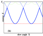
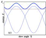
Figure 1: Schematic figure illustrating the formation of the peak of the function $\Delta E^{(-)}_{sm}(\omega_{f})$: (a) $\omega_{f}=\omega_{\max}$; (b) $\omega_{f}<\omega_{\max}$; (c) $\omega_{f}>\omega_{\max}$. The relevant (lower) GSS curve is shown by the dotted line. The relevant trajectories of the resonance Hamiltonian are shown by solid lines. The lower boundary of the layer is marked by a thick solid line: in (a) and (b) the lower boundary is formed by the lower part of the resonance separatrix while, in (c) it is formed by the resonance trajectory tangent to the GSS curve. The dashed line marks, for a given $\omega_{f}$, the maximal deviation of the lower boundary from the separatrix energy $E_{s}$.

The boundary of the SM chaotic layer is formed by those parts of the SM chaotic trajectory which deviate from the separatrix more than others. It follows from the structure of the chaotic trajectory described above that the upper/lower boundary of the SM chaotic layer is formed in one of the two following ways pre2008 ; proceedings : (i) if there exists a self-intersecting resonance trajectory (in other words, the resonance separatrix) the lower/upper part of which (i.e. the part situated below/above the self-intersection) touches or intersects the upper/lower GSS curve while the upper/lower part does not, then the upper/lower boundary of the layer is formed by the upper/lower part of this self-intersecting trajectory (Figs. 1(a) and 1(b)); (ii) otherwise the boundary is formed by the resonance trajectory tangent to the GSS curve (Fig. 1(c)). It is shown below that, in both cases, the variation of the energy along the resonance trajectory is larger than the separatrix split $\delta$ by a logarithmically large factor $\propto\ln(1/h)$. Therefore, over the boundary of the SM chaotic layer the largest deviation of the energy from the separatrix value, $\Delta E^{(\pm)}_{sm}$, may be taken, in the leading-order approximation, to be equal to the largest variation of the energy along the resonance trajectory forming the boundary, while the latter trajectory can be entirely described within the resonance Hamiltonian formalism.

Finally, we mention that, as is obvious from the above description of the boundary, $\Delta E^{(\pm)}_{sm}\equiv\Delta E^{(\pm)}_{sm}(\omega_{f})$ possesses a local maximum $\Delta E^{(\pm)}_{\max,sm}$ at $\omega_{f}$ for which the resonance separatrix just touches the corresponding GSS curve (see Fig. 1(a)).

3 Single-Separatrix Chaotic Layer

It is clear from Sec. 2 above that $\Delta E^{(\pm)}_{\max,sm}$ is equal in leading order to the width $\Delta E_{NR}$ of the nonlinear resonance which touches the separatrix. In Sec. 3.1 below, we roughly estimate $\Delta E_{NR}$ in order to classify two different types of systems. Secs. 3.2 and 3.3 present the accurate leading-order asymptotic theory for the two types of systems. The next-order correction is estimated in Sec. 3.4, while a discussion is presented in Sec. 3.5.

3.1 Rough estimates. Classification of systems.

Let us roughly estimate $\Delta E_{NR}$: it will turn out that it is thus possible to classify all systems into two different types. With this aim, we expand the perturbation $V$ into two Fourier series in $t$ and in $\psi$ respectively:

$$V\equiv\frac{1}{2}\sum_{l}V^{(l)}(E,\psi){\rm e}^{-{\rm i}l\omega_{f}t}+{\rm c.c.}\equiv\frac{1}{2}\sum_{l,k}V^{(l)}_{k}(E){\rm e}^{{\rm i}(k\psi-l\omega_{f}t)}+{\rm c.c.}$$ (8)

As in standard nonlinear resonance theory Chirikov:79 ; lichtenberg_lieberman ; Zaslavsky:1991 ; zaslavsky:1998 ; zaslavsky:2005 , we single out the relevant (for a given peak) numbers $K$ and $L$ for the blind indices $k$ and $l$ respectively, and denote the absolute value of $V^{(L)}_{K}$ as $V_{0}$:

$$V_{0}(E)\equiv|V^{(L)}_{K}(E)|.$$ (9)

To estimate the width of the resonance roughly, we use the pendulum approximation of resonance dynamics Chirikov:79 ; lichtenberg_lieberman ; Zaslavsky:1991 ; zaslavsky:1998 ; zaslavsky:2005 ; abdullaev :

$$\Delta E_{NR}\sim\sqrt{8hV_{0}\omega_{f}/|{\rm d}\omega/{\rm d}E|}.$$ (10)

This approximation assumes constancy of ${\rm d}\omega/{\rm d}E$ in the resonance range of energies, which is not the case here: in reality, $\omega(E)\propto 1/\ln(1/|E-E_{s}|)$ in the vicinity of the separatrix ZF:1968 ; Chirikov:79 ; lichtenberg_lieberman ; Zaslavsky:1991 ; zaslavsky:1998 ; zaslavsky:2005 ; abdullaev ; treschev ; shevchenko:1998 ; vecheslavov ; shevchenko ; pre2008 ; proceedings , so that the relevant derivative $|{\rm d}\omega/{\rm d}E|\sim(\omega_{r}^{(\pm)})^{2}/(\omega_{0}|E-E_{s}|)$ varies strongly within the resonance range. However, for our rough estimate we may use the maximal value of $|E-E_{s}|$, which is approximately equal to $\Delta E_{NR}$. If $\omega_{f}$ is of the order of $\omega_{r}^{(\pm)}\sim\omega_{0}/\ln(1/h)$, then Eq. (10) reduces to the following approximate asymptotic equation for $\Delta E_{NR}$:

$$\Delta E_{NR}\sim V_{0}(E=E_{s}\pm\Delta E_{NR})h\ln(1/h),\quad\quad h\rightarrow 0.$$ (11)

The asymptotic solution of Eq. (11) depends on $V_{0}(E_{s}\pm\Delta E_{NR})$ as a function of $\Delta E_{NR}$. In this context, all systems can be divided in two types.

• The separatrix of the unperturbed system has two or more saddles while the relevant Fourier coefficient $V^{(L)}\equiv V^{(L)}(E,\psi)$ possesses different values on adjacent saddles. Given that, for $E\rightarrow E_{s}$, the system stays most of time near one of the saddles, the coefficient $V^{(L)}(E\rightarrow E_{s},\psi)$ as a function of $\psi$ is nearly a “square wave”: it oscillates between the values at the different saddles. The relevant $K$ is typically odd and, therefore, $V_{0}(E\rightarrow E_{s})$ approaches a well defined non-zero value. Thus, the quantity $V_{0}(E=E_{s}\pm\Delta E_{NR})$ in Eq. (11) may be approximated by this non-zero limit, and we conclude therefore that

  $$\Delta E_{NR}\propto h\ln(1/h),\quad\quad h\rightarrow 0.$$ (12)

• Either (i) the separatrix of the unperturbed system has a single saddle, or (ii) it has more than one saddle but the perturbation coefficient $V^{(L)}$ is identical for all saddles. Then $V^{(L)}(E\rightarrow E_{s},\psi)$, as a periodic function of $\psi$, significantly differs from its value at the saddle(s) only during a small part of the period in $\psi$: this part is $\sim\omega(E)/\omega_{0}\sim 1/\ln(1/|E_{s}-E|)$. Hence, $V_{0}(E_{s}\pm\Delta E_{NR})\propto 1/\ln(1/\Delta E_{NR})$. Substituting this value in Eq. (11), we conclude that

  $$\Delta E_{NR}\propto h,\quad\quad h\rightarrow 0.$$ (13)

Thus, for systems of type I, the maximum width of the SM chaotic layer is proportional to $h$ times a logarithmically large factor $\propto\ln(1/h)$ while, for systems of type II, it is proportional to $h$ times a numerical factor.

As shown below, the variation of energy in between the instants relevant to the SM is $\sim h$, i.e. much less than $\Delta E_{NR}$ (12) for systems of the type I, and of the same order as $\Delta E_{NR}$ (13) for systems of type II. Therefore, one may expect that the maximum width of the layer for the original Hamiltonian system (1), $\Delta E^{(\pm)}$, is at least roughly approximated by that for the SM, $\Delta E_{sm}^{(\pm)}$, so that the above classification of systems is relevant to $\Delta E^{(\pm)}$ too. This is confirmed both by numerical integration of the equations of motion of the original Hamiltonian system and by the accurate theory presented in the next two sub-sections.

3.2 Asymptotic theory for systems of type I.

For the sake of clarity, we consider a particular example of a type I system; its generalization is straightforward.

We choose an archetypal example: the ac-driven pendulum (sometimes referred to as a pendulum subject to a dipole time-periodic perturbation) Zaslavsky:1991 ; prl2005 ; 13_prime :

$$H=H_{0}+hV,$$ (14)

$$H_{0}=\frac{p^{2}}{2}-\cos(q),\quad\quad V=-q\cos(\omega_{f}t),\quad\quad h\ll 1.$$

Fig. 2 presents the results of numerical simulations for a few values of $h$ and several values of $\omega_{f}$. It shows that: (i) that the function $\Delta E^{(-)}(\omega_{f})$ indeed possesses sharp peaks whose heights greatly exceed the estimates by the heuristic Zaslavsky:1991 , adiabatic E&E:1991 and moderate-frequency treschev theories (see inset); (ii) as predicted by our rough estimates of Sec. 3.1, the 1st peak of $\Delta E^{(-)}(\omega_{f})$ shifts to smaller values of $\omega_{f}$ while its magnitude grows, as $h$ decreases. Below, we develop a leading-order asymptotic theory, in which the parameter of smallness is $1/\ln(1/h)$, and compare it with results of the simulations.

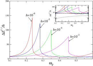
Figure 2: Computer simulations for the ac driven pendulum (14) (an archetypal example of type I): the deviation $\Delta E^{(-)}$ of the lower boundary of the chaotic layer from the separatrix, normalized by the perturbation amplitude $h$, is plotted as a function of the perturbation frequency $\omega_{f}$, for various $h$. The inset presents the same data but with a logarithmic ordinate and with the estimates by the heuristic Zaslavsky:1991 , adiabatic E&E:1991 and moderate-frequency treschev theories. The heuristic estimate is shown by the dotted line: as an example of the heuristic estimate, we use the formula from Zaslavsky:1991 : $\Delta E^{(-)}/h=2\pi\omega_{f}/\cosh(\pi\omega_{f}/2)$. The adiabatic and moderate-frequency estimates are shown by the dashed line: the adiabatic estimate for $\Delta E^{(-)}(\omega_{f})$ is equal approximately to $2\pi$; the estimate following from the results of the work treschev for $\omega_{f}\sim 1$ is of the same order, so that it is schematically represented in the inset in Fig. 2 by the same line as for the adiabatic estimate (dashed line). The inset shows explicitly that the simulation results exceed the estimates of the former theories by 1 or 2 orders of magnitude, over a wide range of frequencies.

Before moving on, we note that the SM (approximated in the relevant case by nonlinear resonance dynamics) considers states of the system only at discrete instants. Apart from the variation of energy within the SM dynamics, a variation of energy in the Hamiltonian system also occurs in between the instants relevant to the SM. Given that $\omega_{f}\ll 1$, this latter variation may be considered in adiabatic approximation and it is of the order of $h$ E&E:1991 ; shevchenko . It follows from the above rough estimates, and from the more accurate consideration below, that the variation of energy within the SM dynamics for systems of type I is logarithmically larger i.e. larger by the factor $\ln(1/h)$. The variation of energy in between the instants relevant to the SM may therefore be neglected to leading-order for systems of type I: $\Delta E^{(-)}\simeq\Delta E^{(-)}_{sm}$. For the sake of notational compactness, we shall henceforth omit the subscript “$sm$” in this subsection.

For the system (14), the separatrix energy is equal to 1, while the asymptotic (for $E\rightarrow E_{s}$) dependence $\omega(E)$ is Zaslavsky:1991 :

$$\omega(E)\simeq\frac{\pi}{\ln(32/|E_{s}-E|)},$$ (15)

$$E_{s}=1,\quad\quad|E_{s}-E|\ll 1.$$

Let us consider the range of energies below $E_{s}$ (the range above $E_{s}$ may be considered in an analogous way) and assume that $\omega_{f}$ is close to an odd multiple of $\omega_{r}^{(-)}$. The nonlinear resonance dynamics of the slow variables in the range of approximately resonant energies may be described as follows pre2008 ; PR (cf. also Chirikov:79 ; lichtenberg_lieberman ; Zaslavsky:1991 ; zaslavsky:1998 ; zaslavsky:2005 ; abdullaev ):

$$\frac{{\rm d}I}{{\rm d}t}=-\frac{\partial{\tilde{H}}(I,{\tilde{\psi}})}{\partial{\tilde{\psi}}},\quad\quad\frac{{\rm d}{\tilde{\psi}}}{{\rm d}t}=\frac{\partial{\tilde{H}}(I,{\tilde{\psi}})}{\partial I},$$ (16)

$$\tilde{H}(I,\tilde{\psi})=\int_{I(E_{s})}^{I}{\rm d}\tilde{I}\;(n\omega-\omega_{f})\;-\;nhq_{n}\cos(\tilde{\psi})$$

$$\quad\;\equiv\;n(E-E_{s})-\omega_{f}(I-I(E_{s}))\;-\;nhq_{n}\cos(\tilde{\psi})\;,$$

$$I\equiv I(E)=\int_{E_{\rm min}}^{E}\frac{{\rm d}\tilde{E}}{\omega(\tilde{E})},\quad\quad E\equiv H_{0}(p,q),$$

$$\tilde{\psi}=n\psi-\omega_{f}t,\quad\quad$$

$$\psi=\pi+{\rm sign}(p)\omega(E)\int^{q}_{q_{\rm min}(E)}\frac{{\rm d}\tilde{q}}{\sqrt{2(E-U(\tilde{q}))}}+2\pi l,$$

$$q_{n}\equiv q_{n}(E)=\frac{1}{2\pi}\int_{0}^{2\pi}\!\!\!\!\!{\rm d}\psi\;q(E,\psi)\cos(n\psi),$$

$$|n\omega-\omega_{f}|\ll\omega,\quad\quad n\equiv 2j-1,\quad\quad j=1,2,3,\ldots,$$

where $I$ and $\psi$ are the canonical variables action and angle respectively Chirikov:79 ; lichtenberg_lieberman ; Zaslavsky:1991 ; zaslavsky:1998 ; zaslavsky:2005 ; abdullaev ; $E_{\rm min}$ is the minimal energy over all $q,p$, $E\equiv H_{0}(p,q)$; $q_{\rm min}(E)$ is the minimum coordinate of the conservative motion with a given value of energy $E$; $l$ is the number of right turning points in the trajectory $[q(\tau)]$ of the conservative motion with energy $E$ and given initial state $(q_{0},p_{0})$.

The resonance Hamiltonian $\tilde{H}(I,\tilde{\psi})$ is obtained in the following way. First, the original Hamiltonian $H$ is transformed to action-angle variables $I-\psi$. Then it is multiplied by $n$ and the term $\omega_{f}I$ is extracted (the latter two operations correspond to the transformation $\psi\rightarrow\tilde{\psi}\equiv n\psi-\omega_{f}t$). Finally, the result is being averaged over time i.e. only the resonance term in the double Fourier expansion of the perturbation is kept (it may be done since the effect of the fast-oscillating terms on the dynamics of slow variables is small: see the estimate of the corrections in Sec. 3.4 below).

Let us derive asymptotic expression for $I(E)$, substituting the asymptotic expression (15) for $\omega(E)$ into the definition of $I(E)$ (16) and carrying out the integration:

$$I(E)\simeq I(E_{s})-\frac{E_{s}-E}{\pi}\left(\ln\left(\frac{32}{E_{s}-E}\right)+1\right).$$ (17)

As for the asymptotic value $q_{n}(E\rightarrow E_{s})$, it can be seen that $q(E\rightarrow E_{s},\psi)$, as a function of $\psi$, asymptotically approaches a “square wave”, oscillating between $-\pi$ and $\pi$, so that, for sufficiently small $j$,

$$q_{2j-1}(E\rightarrow E_{s})\simeq(-1)^{j+1}\frac{2}{2j-1},$$ (18)

$$q_{2j}=0,$$

$$j=1,2,...\ll\frac{\pi}{2\omega(E)}.$$

The next issue is the analysis of the phase space of the resonant Hamiltonian (16). Substituting $\tilde{H}$ (16) into the equations of motion (16), it can be seen that their stationary points have the following values of the slow angle

$$\tilde{\psi}_{+}=\pi,\quad\quad\tilde{\psi}_{-}=0,$$ (19)

while the corresponding action is determined by the equation

$$n\omega-\omega_{f}\mp nh\frac{{\rm d}q_{n}}{{\rm d}I}=0,\quad\quad n\equiv 2j-1,$$ (20)

where the sign “$\mp$”corresponds to $\tilde{\psi}_{\mp}$ (19).

The term $\propto h$ in (20) may be neglected to leading-order (cf. Chirikov:79 ; lichtenberg_lieberman ; Zaslavsky:1991 ; zaslavsky:1998 ; zaslavsky:2005 ; abdullaev ; pre2008 ; PR ), and Eq. (20) reduces to the resonance condition

$$(2j-1)\omega(E_{r}^{(j)})=\omega_{f},$$ (21)

the lowest-order solution of which is

$$E_{s}-E_{r}^{(j)}\simeq 32\exp\left(-\frac{(2j-1)\pi}{\omega_{f}}\right).$$ (22)

Eqs. (19) and (22) together with (17) explicitly determine the elliptic and hyperbolic points of the Hamiltonian (16). The hyperbolic point is often referred to as a “saddle” and corresponds to $\tilde{\psi}_{+}$ or $\tilde{\psi}_{-}$ in (19) for even or odd $j$ respectively. The saddle point generates the resonance separatrix. Using the asymptotic relations (17) and (18), we find that the resonance Hamiltonian (16) takes the following asymptotic value in the saddle:

$$\tilde{H}_{saddle}\simeq\frac{E_{s}-E_{r}^{(j)}}{\pi}\omega_{f}-2h$$

$$\quad\quad\quad\simeq\frac{\omega_{f}}{\pi}32\exp\left(-\frac{\pi(2j-1)}{\omega_{f}}\right)-2h.$$ (23)

The second asymptotic equality in (23) takes into account the relation (22).

As explained in Sec. 2 above, $\Delta E^{(-)}(\omega_{f})$ possesses a local maximum at $\omega_{f}$ for which the resonance separatrix is tangent to the lower GSS curve (Fig. 1(a)). For the relevant frequency range $\omega_{f}\rightarrow 0$, the separatrix split (which represents the maximum deviation of the energy along the GSS curve from $E_{s}$) approaches the following value Zaslavsky:1991 in the asymptotic limit $h\rightarrow 0$

$$\delta\simeq 2\pi h,\quad\quad\omega_{f}\ll 1.$$ (24)

As shown below, the variation of energy along the relevant resonance trajectories is much larger. Therefore, in the leading-order approximation, the GSS curve may simply be replaced by the separatrix of the unperturbed system i.e. by the horizontal line $E=E_{s}$ or, equivalently, $I=I(E_{s})$. Then the tangency occurs at $\tilde{\psi}$, shifted from the saddle by $\pi$, so that the condition of tangency is written as

$$\tilde{H}_{saddle}=\tilde{H}(I=I(E_{s}),\tilde{\psi}=\tilde{\psi}_{saddle}+\pi)\equiv 2h.$$ (25)

Substituting here $\tilde{H}_{saddle}$ (23), we finally obtain the following transcendental equation for $\omega_{\max}^{(j)}$:

$$x\exp(x)=\frac{8(2j-1)}{h},\quad\quad x\equiv\frac{(2j-1)\pi}{\omega_{\max}^{(j)}}.$$ (26)

Fig. 3(b) demonstrates the excellent agreement between Eq. (26) and simulations of the Hamiltonian system over a wide range of $h$.

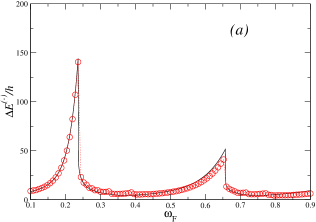
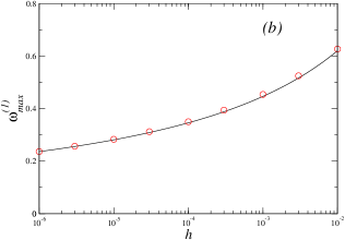
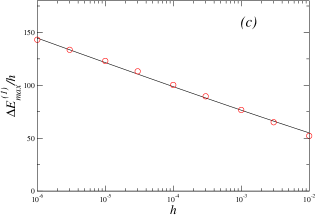
Figure 3: An archetypal example of a type I system: the ac-driven pendulum (14). Comparison of theory (solid lines) and simulations (circles) for: (a) the deviation $\Delta E^{(-)}(\omega_{f})$ of the lower boundary of the chaotic layer from the separatrix, normalized by the perturbation amplitude $h$, as a function of the perturbation frequency $\omega_{f}$, for $h=10^{-6}$; the theory is from Eqs. (26), (31), (32), (38), (39) and (41) (note the discontinuous drop by the factor e from the maximum to the right wing). (b) The frequency of the 1st maximum in $\Delta E^{(-)}(\omega_{f})$ as a function of $h$; the theory is from Eq. (26). (c) The 1st maximum in $\Delta E^{(-)}(\omega_{f})/h$ as a function of $h$; the theory is from Eqs. (34) and (26).

In the asymptotic limit $h\rightarrow 0$, the lowest-order explicit solution of Eq. (26) is

$$\omega_{\max}^{(j)}\simeq\frac{(2j-1)\pi}{\ln\left(\frac{8(2j-1)}{h}\right)},\quad\quad j=1,2,...\ll\ln\left(\frac{1}{h}\right).$$ (27)

As follows from Eq. (26), the value of $E_{s}-E_{r}^{(j)}$ (22) for $\omega_{f}=\omega_{\max}^{(j)}$ is

$$E_{s}-E_{r}^{(j)}(\omega_{f}=\omega_{\max}^{(j)})=\frac{4\pi h}{\omega_{\max}^{(j)}}.$$ (28)

Its leading-order expression is:

$$E_{s}-E_{r}^{(j)}(\omega_{f}=\omega_{\max}^{(j)})\simeq\frac{4h}{2j-1}\ln\left(\frac{8(2j-1)}{h}\right),\quad\quad h\rightarrow 0.$$ (29)

If $\omega_{f}\leq\omega_{\max}^{(j)}$ then, in the chaotic layer, the largest deviation of energy from the separatrix value corresponds to the minimum energy $E_{\min}^{(j)}$ on the nonlinear resonance separatrix (Fig. 1(a,b)), which occurs at $\tilde{\psi}$ shifted by $\pi$ from the saddle. The condition of equality of $\tilde{H}$ at the saddle and at the minimum of the resonance separatrix is written as

$$\tilde{H}_{saddle}=\tilde{H}(I(E_{\min}^{(j)}),\tilde{\psi}_{saddle}+\pi).$$ (30)

Let us seek its asymptotic solution in the form

$$E_{s}-E_{\min}^{(j)}\equiv\Delta E_{l}^{(j)}=(1+y)(E_{s}-E_{r}^{(j)})\simeq(1+y)32\exp\left(-\frac{\pi(2j-1)}{\omega_{f}}\right),$$

$$y\stackrel{{\scriptstyle>}}{{\sim}}1.$$ (31)

Substituting (31) and (23) into Eq. (30), we obtain for $y$ the following transcendental equation:

$$(1+y)\ln(1+y)-y=\frac{h}{8(2j-1)}x_{f}\exp(x_{f}),$$ (32)

$$x_{f}\equiv\frac{\pi(2j-1)}{\omega_{f}},\quad\quad\omega_{f}\leq\omega_{\max}^{(j)},\quad\quad y>0,$$

where $\omega_{\max}^{(j)}$ is given by Eq. (26).

Eqs. (31) and (32) describe the left wing of the $j$-th peak of $\Delta E^{(-)}(\omega_{f})$. Fig. 3(a) demonstrates the good agreement between our analytic theory and simulations for the Hamiltonian system.

It follows from Eq. (26) that Eq. (32) for $\omega_{f}=\omega_{\max}^{(j)}$ reduces to the relation $\ln(1+y)=1$, i.e.

$$1+y(\omega_{\max}^{(j)})={\rm e}.$$ (33)

It follows from Eqs. (33), (31) and (28) that the maximum for a given peak is:

$$\Delta E^{(j)}_{\max}\equiv E_{s}-E^{(j)}_{\min}(\omega_{\max}^{(j)})=\frac{4\pi{\rm e}h}{\omega_{\max}^{(j)}}.$$ (34)

Fig. 3(c) shows the excellent agreement of this expression with our simulations of the Hamiltonian system over a wide range of $h$.

The leading-order expression for $\Delta E^{(j)}_{\max}$ is:

$$\Delta E^{(j)}_{\max}\simeq\frac{4{\rm e}h}{2j-1}\ln(8(2j-1)/h),\quad\quad h\rightarrow 0,$$ (35)

which confirms the rough estimate (12).

As $\omega_{f}$ decreases, it follows from Eq. (32) that $y$ increases exponentially sharply. In order to understand how $\Delta E_{l}^{(j)}$ decreases upon decreasing $\omega_{f}$, it is convenient to rewrite Eq. (31) re-expressing the exponent by means of Eq. (32):

$$\Delta E_{l}^{(j)}(\omega_{f})=\frac{4\pi h}{\omega_{f}(\ln(1+y)-y/(1+y))}.$$ (36)

It follows from Eqs. (32) and (36) that $\Delta E_{l}^{(j)}$ decreases power-law-like when $\omega_{f}$ is decreased. In particular, $\Delta E_{l}^{(j)}\propto 1/(\omega_{\max}^{(j)}-\omega_{f})$ at the far part of the wing.

As for the right wing of the peak, i.e. for $\omega_{f}>\omega_{\max}^{(j)}$, over the chaotic layer, the largest deviation of energy from the separatrix value corresponds to the minimum of the resonance trajectory tangent to the GSS curve (Fig. 1(c)). The value of $\tilde{\psi}$ at the minimum coincides with $\tilde{\psi}_{saddle}$. In the leading-order approximation, the GSS curve may be replaced by the horizontal line $I=I(E_{s})$, so that the tangency occurs at $\tilde{\psi}=\tilde{\psi}_{saddle}+\pi$. Then the energy at the minimum $E_{\min}^{(j)}$ can be found from the equation

$$\tilde{H}(I(E_{s}),\tilde{\psi}_{saddle}+\pi)=\tilde{H}(I(E_{\min}^{(j)}),\tilde{\psi}_{saddle})$$ (37)

Let us seek its asymptotic solution in the form

$$E_{s}-E_{\min}^{(j)}\equiv\Delta E_{r}^{(j)}=z(E_{s}-E_{r}^{(j)})\simeq z32\exp\left(-\frac{\pi(2j-1)}{\omega_{f}}\right)$$

$$0<z<1,\quad\quad z\sim 1.$$ (38)

Substituting (38) into (37), we obtain for $z$ the following transcendental equation:

$$z(1+\ln(1/z))=\frac{h}{8(2j-1)}x_{f}\exp(x_{f})$$ (39)

$$x_{f}\equiv\frac{\pi(2j-1)}{\omega_{f}},\quad\quad\omega_{f}>\omega_{\max}^{(j)},\quad\quad 0<z<1,$$

where $\omega_{\max}^{(j)}$ is given by Eq. (26). Eqs. (38) and (39) describe the right wing of the $j$-th peak of $\Delta E^{(-)}(\omega_{f})$. Fig. 3(a) demonstrates the good agreement between our analytic theory and simulations.

It follows from Eq. (26) that the solution of Eq. (39) for $\omega_{f}\rightarrow\omega_{\max}^{(j)}$ is $z\rightarrow 1$, so the right wing starts from the value given by Eq. (28) (or, approximately, by Eq. (29)). Expressing the exponent in (38) from (39), we obtain the following equation

$$\Delta E_{r}^{(j)}(\omega_{f})=\frac{4\pi h}{\omega_{f}(1+\ln(1/z))}.$$ (40)

It follows from Eqs. (39) and (40) that $\Delta E_{r}^{(j)}$ decreases power-law-like for increasing $\omega_{f}$. In particular, $\Delta E_{r}^{(j)}\propto 1/(\omega_{f}-\omega_{\max}^{(j)})$ in the far part of the wing. Further analysis of the asymptotic shape of the peak is presented in Sec. 3.5 below.

Beyond the peaks, the function $\Delta E^{(-)}(\omega_{f})$ is logarithmically small in comparison with the maxima of the peaks. The functions $\Delta E^{(j)}_{l}(\omega_{f})$ and $\Delta E^{(j)}_{r}(\omega_{f})$ in the ranges beyond the peaks are also logarithmically small. Hence, nearly any function of $\Delta E^{(j)}_{r}(\omega_{f})$ and $\Delta E^{(j+1)}_{l}(\omega_{f})$ which is close to $\Delta E^{(j)}_{r}(\omega_{f})$ in the vicinity of $\omega_{\max}^{(j)}$ and to $\Delta E^{(j+1)}_{l}(\omega_{f})$ in the vicinity of $\omega_{\max}^{(j+1)}$ while being sufficiently small beyond the peaks may be considered as an approximation of the function $\Delta E^{(-)}(\omega_{f})$ to logarithmic accuracy with respect to the maxima of the peaks, $\Delta E_{\max}^{(j)}$ and $\Delta E_{\max}^{(j+1)}$, in the whole range $[\omega_{\max}^{(j)},\omega_{\max}^{(j+1)}]$. One of the easiest options is the following:

$$\Delta E^{(-)}(\omega_{f})=\Delta E^{(1)}_{l}(\omega_{f})\;\quad\quad\quad\quad\quad\quad\quad\quad\quad\quad{\rm for}\quad\omega_{f}<\omega_{\max}^{(1)},$$

$$\Delta E^{(-)}(\omega_{f})=\max\{\Delta E^{(j)}_{r}(\omega_{f}),\Delta E^{(j+1)}_{l}(\omega_{f})\}\quad\quad{\rm for}\quad\omega_{\max}^{(j)}<\omega_{f}<\omega_{\max}^{(j+1)},$$

$$j=1,2,...\ll\frac{\pi}{2\omega_{\max}^{(1)}}.$$ (41)

We used this function in Fig. 3(a), and the analogous one will also be used in the other cases.

In fact, the theory may be generalized in such a way that Eq. (41) would approximate $\Delta E^{(-)}(\omega_{f})$ well in the ranges far beyond the peaks with logarithmic accuracy, even with respect to $\Delta E^{(-)}(\omega_{f})$ itself rather than to $\Delta E_{\max}^{(j)}$ only (cf. the next section). However, we do not do this in the present case, being interested primarily in the leading-order description of the peaks.

Finally, we demonstrate in Fig. 4 that the lowest-order theory describes the boundary of the layers quite well, even in the Poincaré section rather than only in energy/action.

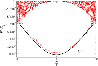
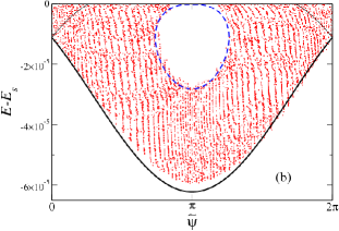
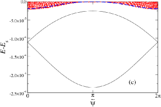
Figure 4: Some characteristic Poincaré sections in the $2\pi$-interval of the energy-angle plane for the system (14) with $h=10^{-6}$ and $\omega_{f}$ equal to: (a) 0.236 (maximum), (b) 0.21 (left wing), (c) 0.25 (right wing). Results of the numerical integration of the equations of motion for the original Hamiltonian (14) are shown by (red) dots. The NR separatrix calculated in the leading-order approximation (i.e. by the integration of the resonant equations of motion (16) in which $\omega(E)$, $I(E)$ and $q_{1}(E)$ are approximated by the explicit formulæ (15), (17) and (18) respectively) is drawn by the (black) solid line. The NR trajectory (calculated in the leading-order approximation) tangent to the line $E=E_{s}$ is drawn by the (blue) dashed line. The outer boundary (marked by a thicker line) is approximated by: the lower part of the NR separatrix in cases (a) and (b), and by the tangent NR trajectory in case (c) The boundary of the island of stability in the cases (a) and (b) is approximated by the tangent NR trajectory (which coincides in the case (a) with the NR separatrix).

3.3 Asymptotic theory for systems of type II.

We consider two characteristic examples of type II systems, corresponding to the classification given in Sec. 3.1. As an example of a system where the separatrix of the unperturbed system possesses a single saddle, we consider an ac-driven Duffing oscillator abdullaev ; gelfreich ; treschev ; soskin2000 . As an example of the system where the separatrix possesses more than one saddle, while the perturbation takes equal values at the saddles, we consider a pendulum with an oscillating suspension point abdullaev ; gelfreich ; treschev ; shevchenko:1998 ; shevchenko . The treatment of these cases is similar in many respects to that presented in Sec. 3.2 above. So, we present it in less detail, emphasizing the differences.

AC-driven Duffing oscillator.

Consider the following archetypal Hamiltonian abdullaev ; gelfreich ; treschev ; soskin2000 :

$$H=H_{0}+hV,$$ (42)

$$H_{0}=\frac{p^{2}}{2}-\frac{q^{2}}{2}+\frac{q^{4}}{4},\quad\quad V=-q\cos(\omega_{f}t),\quad\quad h\ll 1.$$

The asymptotic dependence of $\omega(E)$ on $E$ for $E$ below the separatrix energy $E_{s}=0$ is the following abdullaev ; physica1985

$$\omega(E)\simeq\frac{2\pi}{\ln(16/(E_{s}-E))},$$ (43)

$$E_{s}=0,\quad\quad 0<E_{s}-E\ll 1.$$

Correspondingly, the resonance values of energies (determined by the condition analogous to (21)) are

$$E_{s}-E_{r}^{(j)}=16\exp\left(-\frac{2\pi j}{\omega_{f}}\right),\quad\quad j=1,2,3,...$$ (44)

The asymptotic dependence of $I(E)$ is

$$I(E)\simeq I(E_{s})-\frac{E_{s}-E}{2\pi}\left(\ln\left(\frac{16}{E_{s}-E}\right)+1\right).$$ (45)

The nonlinear resonance dynamics is described by the resonance Hamiltonian $\tilde{H}$ which is identical in form to Eq. (16). Obviously, the actual dependences $\omega(E)$ and $I(E)$ are given by Eq. (43) and (45) respectively. The most important difference is in $q_{j}(E)$: instead of a non-zero value (see (18)), it approaches 0 as $E\rightarrow E_{s}$. Namely, it is $\propto\omega(E)$ abdullaev ; physica1985 :

$$q_{j}(E)\simeq\frac{1}{\sqrt{2}}\omega(E),\quad\quad j=1,2,...\ll\frac{\pi}{\omega(E)},$$ (46)

i.e. $q_{j}$ is much smaller than in systems of type I (cf. (18)). Due to this, the resonance is “weaker”. At the same time, the separatrix split $\delta$ is also smaller, namely $\sim h\omega_{f}$ (cf. pre2008 ) rather than $\sim h$ as for the systems of type I. That is why the separatrix chaotic layer is still dominated by resonance dynamics while the matching of the separatrix map and nonlinear resonance dynamics is still valid in the asymptotic limit $h\rightarrow 0$ pre2008 .

Similarly to the previous section, we find the value of $\tilde{H}$ in the saddle in the leading-order approximation:

$$\tilde{H}_{saddle}\simeq\omega_{f}\left(\frac{E_{s}-E_{r}^{(j)}}{2\pi}-\frac{h}{\sqrt{2}}\right),$$ (47)

where $E_{s}-E_{r}^{(j)}$ is given in (44).

As before, the maximum width of the layer corresponds to $\omega_{f}$, for which the resonance separatrix is tangent to the GSS curve (Fig. 1(a)). It can be shown pre2008 that the angle of tangency asymptotically approaches $\tilde{\psi}_{saddle}+\pi=\pi$ while the energy still lies in the resonance range. Here $\omega(E)\approx\omega_{r}^{(-)}\approx\omega_{f}/j$. Using the expressions for $\tilde{H}(E,\tilde{\psi})$ (cf. (16)), $I(E)$ (45), $q_{j}(E)$ (46), and taking into account that in the tangency $E<\delta\sim h\omega_{f}\ll h$, to leading-order the value of $\tilde{H}$ at the tangency reads

$$\tilde{H}_{tangency}\simeq\omega_{f}\frac{h}{\sqrt{2}}.$$ (48)

Allowing for Eqs. (47) and (48), the condition for the maximum, $\tilde{H}_{saddle}=\tilde{H}_{tangency}$, reduces to

$$E_{s}-E_{r}^{(j)}(\omega_{\max}^{(j)})\simeq 2\pi\sqrt{2}h.$$ (49)

Thus these values $E_{s}-E_{r}^{(j)}$ are logarithmically smaller than the corresponding values (28) for systems of type I.

The values of $\omega_{f}$ corresponding to the maxima of the peaks in $\Delta E^{(-)}(\omega_{f})$ are readily obtained from (49) and (44):

$$\omega_{\max}^{(j)}\simeq\frac{2\pi j}{\ln(4\sqrt{2}/(\pi h))},\quad\quad j=1,2,...\ll\ln(1/h).$$ (50)

The derivation to leading order of the shape of the peaks for the chaotic layer of the separatrix map, i.e. within the nonlinear resonance (NR) approximation, is similar to that for type I. So, we present only the results, marking them with the subscript “$NR$”.

The left wing of the $j$th peak of $\Delta E^{(-)}_{NR}(\omega_{f})$ is described by the function

$$\Delta E^{(j)}_{l,NR}(\omega_{f})=16(1+y)\exp\left(-\frac{2\pi j}{\omega_{f}}\right)\equiv\frac{2\pi\sqrt{2}h}{\ln(1+y)-y/(1+y)},$$ (51)

$$\omega_{f}\leq\omega_{\max}^{(j)},$$

where $y$ is the positive solution of the transcendental equation

$$(1+y)\ln(1+y)-y=\frac{\pi h}{4\sqrt{2}}\exp\left(\frac{2\pi j}{\omega_{f}}\right),\quad\quad y>0.$$ (52)

In common with the type I case, $1+y(\omega_{\max}^{(j)})={\rm e}$, so that

$$\Delta E^{(j)}_{\max,NR}={\rm e}(E_{s}-E_{r}^{(j)}(\omega_{\max}^{(j)}))\simeq 2\pi{\rm e}\sqrt{2}h.$$ (53)

Eq. (53) confirms the rough estimate (13). The right wing of the peak is described by the function

$$\Delta E^{(j)}_{r,NR}(\omega_{f})=16z\exp\left(-\frac{2\pi j}{\omega_{f}}\right)\equiv\frac{2\pi\sqrt{2}h}{1+\ln(1/z)},$$ (54)

$$\omega_{f}>\omega_{\max}^{(j)},$$

where $z<1$ is the solution of the transcendental equation

$$z(1+\ln(1/z))=\frac{\pi h}{4\sqrt{2}}\exp\left(\frac{2\pi j}{\omega_{f}}\right),\quad\quad 0<z<1.$$ (55)

As in the type I case, $z(\omega_{f}\rightarrow\omega_{\max}^{(j)})\rightarrow 1$.

It follows from Eqs. (49) and (53) that the typical variation of energy within the nonlinear resonance dynamics (that approximates the separatrix map dynamics) is $\propto h$. For the Hamiltonian system, the variation of energy in between the discrete instants corresponding to the separatrix map Zaslavsky:1991 ; zaslavsky:1998 ; zaslavsky:2005 ; abdullaev ; pre2008 ; vered is also $\propto h$. Therefore, unlike the type I case, one needs to take it into account even at the leading-order approximation. Let us consider the right well of the Duffing potential (the results for the left well are identical), and denote by $t_{k}$ the instant at which the energy $E$ at a given $k$-th step of the separatrix map is taken: it corresponds to the beginning of the $k$-th pulse of velocity Zaslavsky:1991 ; pre2008 i.e. the corresponding $q$ is close to a left turning point $q_{ltp}$ in the trajectory $[q(\tau)]$. Let us also take into account that the relevant frequencies are small so that the adiabatic approximation may be used. Thus, the change of energy from $t_{k}$ up to a given instant $t$ during the following pulse of velocity ($t-t_{k}\sim 1$) may be calculated as

$$\Delta E=\int_{t_{k}}^{t}{\rm d}\tau\dot{q}h\cos(\omega_{f}\tau)\simeq h\cos(\omega_{f}t_{k})\int_{t_{k}}^{t}{\rm d}\tau\dot{q}$$

$$\quad\quad=h\cos(\omega_{f}t_{k})(q(t)-q_{ltp})$$ (56)

For the motion near the separatrix, the velocity pulse corresponds approximately to $\psi=0$ (see the definition of $\psi$ (16)). Thus, the corresponding slow angle is $\tilde{\psi}\equiv j\psi-\omega_{f}t_{k}\simeq-\omega_{f}t_{k}$.

For the left wing of the peak of $\Delta E^{(-)}(\omega_{f})$ (including also the maximum of the peak), the boundary of the chaotic layer of the separatrix map is formed by the lower part of the NR separatrix. The minimum energy along this separatrix occurs at $\tilde{\psi}=\pi$. Taking this into account, and also noting that $\tilde{\psi}\simeq-\omega_{f}t_{k}$, we conclude that $\cos(\omega_{f}t_{k})\simeq-1$. So, $\Delta E\leq 0$, i.e. it does lower the minimum energy of the layer of the Hamiltonian system. The maximum reduction occurs at the right turning point $q_{rtp}$:

$$\max(|\Delta E|)\simeq h(q_{rtp}-q_{ltp})=\sqrt{2}h.$$ (57)

We conclude that the left wing of the $j$-th peak is described as follows:

$$\Delta E_{l}^{(j)}(\omega_{f})\simeq\Delta E_{l,NR}^{(j)}(\omega_{f})+\sqrt{2}h,\quad\quad\omega_{f}\leq\omega_{\max}^{(j)},$$ (58)

where $\Delta E_{l,NR}^{(j)}(\omega_{f})$ is given by Eqs. (51)-(52). In particular, the maximum of the peak is:

$$\Delta E^{(j)}_{\max}\simeq(2\pi{\rm e}+1)\sqrt{2}h\approx 25.6h.$$ (59)

For the right wing of the peak, the minimum energy of the layer of the separatrix map occurs when $\tilde{\psi}$ coincides with $\tilde{\psi}_{saddle}$ (Fig. 1(c)) i.e. is equal to 0. As a result, $\cos(\omega_{f}t_{k})\simeq 1$ and, hence, $\Delta E\geq 0$. So, this variation cannot lower the minimum energy of the layer for the main part of the wing, i.e. for $\omega_{f}\leq\omega_{bend}^{(j)}$ where $\omega_{bend}^{(j)}$ is defined by the condition $\Delta E_{r,NR}^{(j)}=\max(|\Delta E|)\equiv\sqrt{2}h$. For $\omega_{f}>\omega_{bend}^{(j)}$, the minimal energy in the layer occurs at $\tilde{\psi}=\pi$, and it is determined exclusively by the variation of energy during the velocity pulse (the NR contribution is close to zero at such $\tilde{\psi}$). Thus, we conclude that there is a bending of the wing at $\omega_{f}=\omega_{bend}^{(j)}$:

$$\Delta E_{r}^{(j)}(\omega_{f})=\Delta E_{r,NR}^{(j)}(\omega_{f}),\quad\quad\omega_{\max}^{(j)}<\omega_{f}\leq\omega_{bend}^{(j)},$$

$$\Delta E_{r}^{(j)}(\omega_{f})=\sqrt{2}h,\quad\quad\quad\quad\quad\omega_{f}\geq\omega_{bend}^{(j)},$$

$$\omega_{bend}^{(j)}=\frac{2\pi j}{\ln(8\sqrt{2}/h)+1-2\pi},$$ (60)

where $\Delta E_{r,NR}^{(j)}(\omega_{f})$ is given by Eqs. (54) and (55).

Analogously to the previous case, $\Delta E^{(-)}(\omega_{f})$ may be approximated over the whole frequency range by Eq. (41) with $\Delta E_{l}^{(j)}$ and $\Delta E_{r}^{(j)}$ given by Eqs. (58) and (60) respectively. Moreover, unlike the previous case, the theory also describes accurately the range far beyond the peaks: $\Delta E^{(-)}$ is dominated in this range by the velocity pulse contribution $\Delta E$, which is accurately taken into account both by Eqs. (58) and (60).

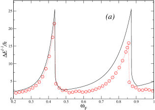
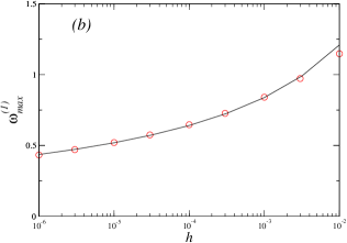
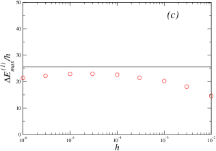
Figure 5: An archetypal example of a type II system: the ac driven Duffing oscillator (42). Comparison of theory (solid lines) and simulations (circles): (a) the deviation $\Delta E^{(-)}(\omega_{f})$ of the lower boundary of the chaotic layer from the separatrix, normalized by the perturbation amplitude $h$, as a function of the perturbation frequency $\omega_{f}$, for $h=10^{-6}$; the theory is from Eqs. (41), (50), (51), (52), (54), (55), (58) and (60) (note the discontinuous drop from the maximum to the right wing); (b) the frequency of the 1st maximum in $\Delta E^{(-)}(\omega_{f})$ as a function of $h$; the theory is from Eq. (50); (c) the 1st maximum in $\Delta E^{(-)}(\omega_{f})/h$ as a function of $h$; the theory is from Eq. (59).

Fig. 5 shows very reasonable agreement between the theory and simulations, especially for the 1st peak.

Pendulum with an oscillating suspension point

Consider the archetypal Hamiltonian abdullaev ; gelfreich ; treschev ; shevchenko:1998 ; shevchenko

$$H=H_{0}+hV,$$

$$H_{0}=\frac{p^{2}}{2}+\cos(q),\quad\quad V=-\cos(q)\cos(\omega_{f}t),\quad\quad h\ll 1.$$ (61)

Though the treatment is similar to that used in the previous case, there are also characteristic differences. One of them is the following: although the resonance Hamiltonian is similar to the Hamiltonian (16), instead of the Fourier component of the coordinate, $q_{n}$, there should be the Fourier component of $\cos(q)$, $V_{n}$, which can be shown to be:

$$V_{2j}\simeq(-1)^{j+1}\frac{4}{\pi}\omega(E),\quad\quad E_{s}-E\ll 1,$$ (62)

$$V_{2j-1}=0,$$

$$j=1,2,...\ll\frac{2\pi}{\omega(E)},\quad\quad V_{n}\equiv\frac{1}{2\pi}\int_{0}^{2\pi}{\rm d}\psi\cos(q)\cos(n\psi).$$

The description of the chaotic layer of the separatrix map at the lowest order, i.e. within the NR approximation, is similar to that for the ac-driven Duffing oscillator. So we present only the results, marking them with the subscript “$NR$”.

The frequency of the maximum of a given $j$-th peak is:

$$\omega_{\max}^{(j)}\simeq\frac{2\pi j}{\ln(4/h)},\quad\quad j=1,2,...\ll\ln(4/h).$$ (63)

This expression agrees well with simulations for the Hamiltonian system (Fig. 6(b)). To logarithmic accuracy, Eq. (63) coincides with the formula following from Eq. (8) of shevchenko:1998 (reproduced in shevchenko as Eq. (21)) taken in the asymptotic limit $h\rightarrow 0$ (or, equivalently, $\omega_{\max}^{(j)}\rightarrow 0$). However, the numerical factor in the argument of the logarithm in the asymptotic formula following from the result of shevchenko:1998 ; shevchenko is half our value: this is because the nonlinear resonance is approximated in shevchenko:1998 ; shevchenko by the conventional pendulum model which is not valid near the separatrix (cf. our Sec. 3.1 above).

The left wing of the $j$th peak of $\Delta E^{(-)}_{NR}(\omega_{f})$ is described by the function

$$\Delta E^{(j)}_{l,NR}(\omega_{f})=32(1+y)\exp\left(-\frac{2\pi j}{\omega_{f}}\right)\equiv\frac{8h}{\ln(1+y)-y/(1+y)},$$ (64)

$$\omega_{f}\leq\omega_{\max}^{(j)},$$

where $y$ is the positive solution of the transcendental equation

$$(1+y)\ln(1+y)-y=\frac{h}{4}\exp\left(\frac{2\pi j}{\omega_{f}}\right),\quad\quad y>0.$$ (65)

Similarly to the previous cases, $1+y(\omega_{\max}^{(j)})={\rm e}$. Hence,

$$\Delta E^{(j)}_{\max,NR}={\rm e}(E_{s}-E_{r}^{(j)}(\omega_{\max}^{(j)}))=8{\rm e}h.$$ (66)

Eq. (66) confirms the rough estimate (13). The right wing of the peak is described by the function

$$\Delta E^{(j)}_{r,NR}(\omega_{f})=32z\exp\left(-\frac{2\pi j}{\omega_{f}}\right)\equiv\frac{8h}{1+\ln(1/z)},$$ (67)

$$\omega_{f}>\omega_{\max}^{(j)},$$

where $z<1$ is the solution of the transcendental equation

$$z(1+\ln(1/z))=\frac{h}{4}\exp\left(\frac{2\pi j}{\omega_{f}}\right),\quad\quad 0<z<1.$$ (68)

Similarly to the previous cases, $z(\omega_{f}\rightarrow\omega_{\max}^{(j)})\rightarrow 1$.

Now consider the variation of energy during a velocity pulse. Though the final result looks quite similar to the case with a single saddle, its derivation has some characteristic differences, and we present it in detail. Unlike the case with a single saddle, the pulse may start close to either the left or the right turning point, and the sign of the velocity in such pulses is opposite Zaslavsky:1991 ; pre2008 . The angle $\psi$ in the pulse is close to $-\pi/2$ or $\pi/2$ respectively. So, let us calculate the change of energy from the beginning of the pulse, $t_{k}$, until a given instant $t$ within the pulse:

$$\Delta E=-\int_{t_{k}}^{t}{\rm d}\tau\dot{q}h\partial V/\partial q=h\int_{t_{k}}^{t}{\rm d}\tau\dot{q}(-\sin(q)\cos(\omega_{f}\tau))$$

$$\simeq h\cos(\omega_{f}t_{k})\int_{t_{k}}^{t}{\rm d}\tau\dot{q}(-\sin(q))\simeq h\cos(\omega_{f}t_{k})(\cos(q(t))-1).$$ (69)

Here, the third equality assumes adiabaticity while the last equality takes into account that the turning points are close to the maxima of the potential i.e. close to a multiple of $2\pi$ (where the cosine is equal to 1).

The quantity $\Delta E$ (69) takes its maximal absolute value at $q=\pi$. So, we shall further consider

$$\Delta E_{\max}=-2h\cos(\omega_{f}t_{k})\equiv-2h\cos(2j\psi_{k}-\tilde{\psi}_{k})=(-1)^{j+1}2h\cos(\tilde{\psi}_{k}).$$ (70)

The last equality takes into account that, as mentioned above, the relevant $\psi_{k}$ is either $-\pi/2$ or $\pi/2$. For the left wing, the value of $\tilde{\psi}$ at which the chaotic layer of the separatrix map possesses a minimal energy corresponds to the minimum of the resonance separatrix. It is equal to $\pi$ or $0$ if the Fourier coefficient $V_{2j}$ is positive or negative, i.e. for odd or even $j$, respectively: see Eq. (63). Thus $\Delta E_{\max}=-2h$ for any $j$ and, therefore, it does lower the minimal energy of the boundary. We conclude that

$$\Delta E_{l}^{(j)}(\omega_{f})\simeq\Delta E_{l,NR}^{(j)}(\omega_{f})+2h,\quad\quad\omega_{f}\leq\omega_{\max}^{(j)},$$ (71)

where $\Delta E_{l,NR}^{(j)}(\omega_{f})$ is given by Eqs. (64)-(65). In particular, the maximum of the peak is:

$$\Delta E^{(j)}_{\max}\simeq(4{\rm e}+1)2h\approx 23.7h.$$ (72)

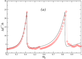
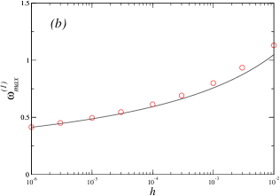
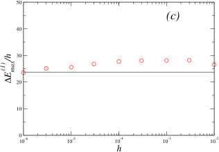
Figure 6: An archetypal example of a type II system: the pendulum with an oscillating suspension point (61). Comparison of theory (solid lines) and simulations (circles): (a) The deviation $\Delta E^{(-)}(\omega_{f})$ of the lower boundary of the chaotic layer from the separatrix, normalized by the perturbation amplitude $h$, as a function of the perturbation frequency $\omega_{f}$, for $h=10^{-6}$; the theory is by Eqs. (41), (63), (64), (65), (67), (68), (71) and (73) (note the dicontinuous drop from the maximum to the right wing). (b) The frequency of the 1st maximum in $\Delta E^{(-)}(\omega_{f})$ as a function of $h$; the theory is from Eq. (63). (c) The 1st maximum in $\Delta E^{(-)}(\omega_{f})/h$ as a function of $h$; the theory is from Eq. (72).

The expression (72) confirms the rough estimate (13) and agrees well with simulations (Fig. 6(c)). At the same time, it differs from the formula which can be obtained from Eq. (10) of shevchenko:1998 (using also Eqs. (1), (3), (8), (9) of shevchenko:1998 ) in the asymptotic limit $h\rightarrow 0$: the latter gives for $\Delta E_{\max}^{(j)}$ the asymptotic value $32h$. Though this result shevchenko:1998 (referred to also in shevchenko ) provides for the correct functional dependence on $h$, it is quantitatively incorrect because (i) it is based on the pendulum approximation of the nonlinear resonance while this approximation is invalid in the vicinity of the separatrix (see the discussion of this issue in Sec. 3.1 above), and (ii) it does not take into account the variation of energy during the velocity pulse.

The right wing, by analogy to the case of the Duffing oscillator, possesses a bend at $\omega_{f}=\omega_{bend}^{(j)}$ where $\Delta E_{r,NR}^{(j)}=|\Delta E_{\max}|\equiv 2h$, corresponding to the shift of the relevant $\tilde{\psi}$ for $\pi$. We conclude that:

$$\Delta E_{r}^{(j)}(\omega_{f})=\Delta E_{r,NR}^{(j)}(\omega_{f}),\quad\quad\omega_{\max}^{(j)}<\omega_{f}\leq\omega_{bend}^{(j)},$$

$$\Delta E_{r}^{(j)}(\omega_{f})=2h,\quad\quad\quad\quad\quad\quad\omega_{f}\geq\omega_{bend}^{(j)},$$

$$\omega_{bend}^{(j)}=\frac{2\pi j}{\ln(16/h)-3},$$ (73)

where $\Delta E_{r,NR}^{(j)}(\omega_{f})$ is given by Eqs. (66) and (67).

Similarly to the previous case, both the peaks and the frequency ranges far beyond the peaks are well approximated by Eq. (41), with $\Delta E_{l}^{(j)}$ and $\Delta E_{r}^{(j)}$ given by Eqs. (71) and (73) respectively (Fig. 6(a)).

3.4 Estimate of the next-order corrections

We have calculated explicitly only the leading term $\Delta E$ in the asymptotic expansion of the chaotic layer width. Explicit calculation of the next-order term $\Delta E^{(next)}$ is possible, but it is rather complicated and cumbersome: cf. the closely related case with two separatrices pre2008 (see also Sec. 4 below). In the present section, where the perturbation amplitude $h$ in the numerical examples is 4 orders of magnitude smaller than that in pre2008 , there is no particular need to calculate the next-order correction quantitatively. Let us estimate it, however, in order to demonstrate that its ratio to the leading term does vanish in the asymptotic limit $h\rightarrow 0$.

We shall consider separately the contribution $\Delta E^{(next)}_{w}$ stemming from the various corrections within the resonance approximation (16) and the contribution $\Delta E^{(next)}_{t}$ stemming from the corrections to the resonance approximation.

The former contribution may be estimated in a similar way to the case considered in pre2008 : it stems, in particular, from the deviation of the GSS curve from the separatrix (this deviation reaches $\delta$ at certain angles: see Eq. (7)) and from the difference between the exact resonance condition (20) and the approximate one (21). It can be shown that the absolute value of the ratio between $\Delta E^{(next)}_{w}$ and the leading term is logarithmically small (cf. pre2008 ):

$$\frac{|\Delta E^{(next)}_{w}|}{\Delta E}\sim\frac{1}{\ln(1/h)}.$$ (74)

Let us turn to the analysis of the contribution $\Delta E^{(next)}_{t}$, i.e. the contribution stemming from the corrections to the resonance Hamiltonian (16). It is convenient to consider separately the cases of the left and right wings of the peak.

As described in Secs. 3.2 and 3.3 above, the left wing corresponds in the leading-order approximation to formation of the boundary of the layer by the separatrix of the resonance Hamiltonian (16). The resonance approximation (16) neglects time-periodic terms while the frequencies of oscillation of these terms greatly exceed the frequency of eigenoscillation of the resonance Hamiltonian (16) around its relevant elliptic point i.e. the elliptic point inside the area limited by the resonance separatrix. As is well known gelfreich ; lichtenberg_lieberman ; treschev ; zaslavsky:1998 ; zaslavsky:2005 ; Zaslavsky:1991 , fast-oscillating terms acting on a system with a separatrix give rise to the onset of an exponentially narrow chaotic layer in place of the separatrix. In the present context, this means that the correction to the maximal action $\tilde{I}$ stemming from fast-oscillating corrections to the resonance Hamiltonian, i.e. $\Delta E^{(next)}_{t}$, is exponentially small, thus being negligible in comparison with the correction $\Delta E^{(next)}_{w}$ (see (74)).

The right wing, described in Secs. 3.2 and 3.3 above, corresponds in leading-order approximation to the formation of the boundary of the layer by the resonance trajectory tangent to the GSS curve. For the part of the right wing exponentially close in frequency to the frequency of the maximum, the tangent trajectory is close to the resonance separatrix, so that the correction stemming from fast-oscillating terms is exponentially small, similarly to the case of the left wing. As the frequency further deviates from the frequency of the maximum, the tangent trajectory further deviates from the resonance separatrix and the correction $\Delta E^{(next)}_{t}$ differs from the exponentially small correction estimated above. It may be estimated in the following way.

It follows from the second-order approximation of the averaging method bogmit that the fast-oscillating terms lead, in the second-order approximation, to the onset of additional terms $h^{2}T_{\tilde{I}}(\tilde{I},\tilde{\psi})$ and $h^{2}T_{\tilde{\psi}}(\tilde{I},\tilde{\psi})$ in the dynamic equations for slow variables $\tilde{I}$ and $\tilde{\psi}$ respectively, where $T_{\tilde{I}}(\tilde{I},\tilde{\psi})$ and $T_{\tilde{\psi}}(\tilde{I},\tilde{\psi})$ are of the order of the power-law-like function of $1/\ln(1/h)$ in the relevant range of $\tilde{I}$. The corresponding correction to the width of the chaotic layer in energy may be expressed as

$$\Delta E^{(next)}_{t}=\int_{t_{\min}}^{t_{\max}}{\rm d}t\;h^{2}T_{\tilde{I}}\omega(\tilde{I}),$$ (75)

where $t_{\min}$ and $t_{\max}$ are instants corresponding to the minimum and maximum deviation of the tangent trajectory from the separatrix of the unperturbed system (cf. Figs. 1(c) and 4(c)). The interval $t_{\max}-t_{\min}$ may be estimated as follows:

$$t_{\max}-t_{\min}\sim\frac{\pi}{|<\dot{\tilde{\psi}}>|},$$ (76)

where $<\dot{\tilde{\psi}}>$ is the value of $\dot{\tilde{\psi}}$ averaged over the tangent trajectory. It follows from (16) that

$$|<\dot{\tilde{\psi}}>|\sim\omega_{f}-\omega(E_{s}-\delta)\sim\frac{\omega(E_{s}-\delta)}{\ln(1/h)}\sim\frac{\omega_{0}}{\ln^{2}(1/h)}.$$ (77)

Taking together Eqs. (75)-(77) and allowing for the fact that $T_{\tilde{I}}$ is of the order of a power-law-like function of $1/\ln(1/h)$, we conclude that

$$\Delta E^{(next)}_{t}\sim h^{2}P(\ln(1/h)),$$ (78)

where $P(x)$ is some power-law-like function.

The value $\Delta E^{(next)}_{t}$ is still asymptotically smaller than the absolute value of the correction within the resonance approximation, $|\Delta E^{(next)}_{w}|$, which is of the order of $h$ or $h/\ln(1/h)$ for systems of type I or type II respectively.

Thus, we conclude that, both for the left and right wings of the peak, (i) the correction $\Delta E^{(next)}_{t}$ is determined by the correction within the resonance approximation $\Delta E^{(next)}_{w}$, and (ii) in the asymptotic limit $h\rightarrow 0$, the overall next-order correction is negligible in comparison with the leading term:

$$\frac{|\Delta E^{(next)}|}{\Delta E}\equiv\frac{|\Delta E^{(next)}_{w}+\Delta E^{(next)}_{t}|}{\Delta E}\approx\frac{|\Delta E^{(next)}_{w}|}{\Delta E}\sim\frac{1}{\ln(1/h)}\stackrel{{\scriptstyle h\rightarrow 0}}{{\longrightarrow}}0.$$ (79)

This estimate well agrees with results in Figs. 3-6.

3.5 Discussion

In this section, we briefly discuss the following issues: (i) the scaled asymptotic shape of the peaks; (ii) peaks in the range of moderate frequencies; (iii) jumps in the amplitude dependence of the layer width; and (iv) chaotic transport; (v) smaller peaks at rational frequencies; (vi) other separatrix maps; (vii) an application to the onset of global chaos.

1. Let us analyse the scaled asymptotic shape of the peaks. We consider first systems of type I. The peaks are then described in the leading-order approximation exclusively within separatrix map dynamics (approximated, in turn, by the NR dynamics). It follows from Eqs. (32), (34), (36), (39) and (40) that most of the peak fir given $j$ can be written in the universal scaled form:

   $$\Delta E^{(j)}(\omega_{f})=\Delta E^{(j)}_{\max}S\left(\frac{\pi(2j-1)}{(\omega_{\max}^{(j)})^{2}}(\omega_{f}-\omega_{\max}^{(j)})\right),$$ (80)

   where the universal function $S(\alpha)$ is strongly asymmetric:

   $$S(\alpha)=\left\{{}^{S_{l}(\alpha)\quad{\rm for}\quad\alpha\leq 0,}_{S_{r}(\alpha)\quad{\rm for}\quad\alpha>0,}\right.$$ (81)

   $$S_{l}(\alpha)=\frac{1}{{\rm e}(\ln(1+y)-y/(1+y))},\quad\quad(1+y)\ln(1+y)-y=\exp(-\alpha),$$

   $$S_{r}(\alpha)=\frac{1}{{\rm e}(1+\ln(1/z))},\quad\quad z(1+\ln(1/z))=\exp(-\alpha).$$

   It is not difficult to show that

   $$S_{l}(\alpha=0)=1,\quad\quad\quad\quad\quad S_{r}(\alpha\rightarrow+0)={\rm e}^{-1},$$ (82)

   $$\frac{{\rm d}S_{l}(\alpha=0)}{{\rm d}\alpha}=1-{\rm e}^{-1},\quad\frac{{\rm d}S_{r}(\alpha\rightarrow+0)}{{\rm d}\alpha}\rightarrow-\infty,$$

   $$\quad\quad\quad\quad\quad S(\alpha\rightarrow\pm\infty)\propto\frac{1}{|\alpha|}.$$

   Thus, the function $S(\alpha)$ is discontinuous at the maximum. To the left of the maximum, it approaches the far part of the wing (which decreases in a power-law-like way) relatively slowly while, to the right of the maximum, the function first drops jump-wise by a factor ${\rm e}$ and then sharply approaches the far part of the wing (which again decreases in a power-law-like way).

   It follows from Eqs. (80), (81), (82) and (27) that the peaks are logarithmically narrow, i.e. the ratio of the half-width of the peak, $\Delta\omega^{(j)}$, to $\omega^{(j)}_{\max}$ is logarithmically small:

   $$\frac{\Delta\omega^{(j)}}{\omega^{(j)}_{\max}}\sim\frac{1}{\ln\left(8(2j-1)/h\right)}.$$ (83)

   We emphasize that the shape (81) is not restricted to the example (14): it is valid for any system of type I.

   For systems of type II, contributions from the NR and from the variation of energy during the pulse of velocity, in relation to their $h$ dependence, are formally of the same order but, numerically, the latter contribution is usually much smaller than the former. Thus, typically, the function (81) approximates well the properly scaled shape of the major part of the peak for systems of type II too.

2. The quantitative theory presented in the paper relates only to the peaks of small order $n$ i.e. in the range of logarithmically small frequencies. At the same time, the magnitude of the peaks is still significant up to frequencies of order of one. This occurs because, for motion close to the separatrix, the order of magnitude of the Fourier coefficients remains the same up to logarithmically large numbers $n$. The shape of the peaks remains the same but their magnitude typically decreases (though in some cases, e.g. in case of the wave-like perturbation lichtenberg_lieberman ; zaslavsky:1998 ; zaslavsky:2005 ; Zaslavsky:1991 it may even increase in some range of frequencies). The quantitative description of this decrease, together with analyses of more sophisticated cases, requires a generalization of our theory.

3. Apart from the frequency dependence of the layer width, our theory is also relevant to amplitude dependence: it describes the jumps soskin2000 in the dependence of the width on $h$ and the transition between the jumps and the linear dependence. The values of $h$ at which the jumps occur, $h_{jump}^{(j)}$, are determined by the same condition that determines $\omega_{\max}^{(j)}$ in the frequency dependence of the width. The formulæ relevant to the left wings of the peaks in the frequency dependence describe the ranges $h>h_{jump}^{(j)}$ while the formulæ relevant to the right wings describe the ranges $h<h_{jump}^{(j)}$.

4. Apart from the description of the boundaries, the approach allows us to describe chaotic transport within the layer. In particular, it allows us to describe quantitatively the effect of the stickiness of the chaotic trajectory to boundaries between the chaotic and regular areas of the phase space zaslavsky:1998 ; zaslavsky:2005 . Moreover, the presence of additional (resonance) saddles should give rise to an additional slowing down of the transport, despite a widening of the area of the phase space involved in the chaotic transport.

5. Our approach can be generalized in order to describe smaller peaks at non-integer rational frequencies i.e. $\omega_{f}\approx n/m\omega_{r}^{(\pm)}$ where $n$ and $m$ are integer numbers.

6. Apart from Hamiltonian systems of the one and a half degrees of freedom and corresponding Zaslavsky separatrix maps, our approach may be useful in the treatment of other chaotic systems and separatrix maps (see treschev for the most recent major review on various types of separatrix maps and related continuous chaotic systems).

7. Finally we note that, apart from systems with a separatrix, our work may be relevant to nonlinear resonances in any system. If the system is perturbed by a weak time-periodic perturbation, then nonlinear resonances arise and their dynamics is described by the model of the auxiliary time-periodically perturbed pendulum Chirikov:79 ; lichtenberg_lieberman ; Zaslavsky:1991 ; zaslavsky:1998 ; zaslavsky:2005 ; abdullaev ; gelfreich . If the original perturbation has a single harmonic, then the effective perturbation of the auxiliary pendulum is necessarily a high-frequency one, and chaotic layers associated with the resonances are exponentially narrow Chirikov:79 ; lichtenberg_lieberman ; Zaslavsky:1991 ; zaslavsky:1998 ; zaslavsky:2005 ; abdullaev ; gelfreich while our results are irrelevant. But, if either the amplitude or the angle of the original perturbation is slowly modulated, or if there is an additional harmonic of a slightly shifted frequency, then the effective perturbation of the auxiliary pendulum is a low-frequency one pre2008 and the layers become much wider while our theoretical approach becomes relevant. It may allow to find optimal parameters of the perturbation for the facilitation of the onset of global chaos associated with the overlap in energy between different-order nonlinear resonances Chirikov:79 : the overlap may be expected to occur at a much smaller amplitude of perturbation in comparison with that one required for the overlap in case of a single-harmonic perturbation.

4 Double-separatrix chaos

There are many problems in physics where an unperturbed Hamiltonian model possesses two or more separatrices. A weak perturbation of the system typically destroys the separatrices, replacing them by thin chaotic layers. As the magnitude of the perturbation grows, the layers become wider and, at some critical value, they merge with each other: this may be described as the onset of global chaos between the separatrices. Such a connection of regions of different separatrices is important for transport in the system.

In the present section, following the paper pre2008 , we consider the characteristic problem of the onset of global chaos between two close separatrices of a 1D Hamiltonian system perturbed by a time-periodic perturbation. As a characteristic example of a Hamiltonian system with two or more separatrices, we use a spatially periodic potential system with two different-height barriers per period (Fig. 7(a)):

$$H_{0}(p,q)=\frac{p^{2}}{2}+U(q),\quad\quad U(q)=\frac{(\Phi-\sin(q))^{2}}{2},\quad\quad\Phi={\rm const}<1.$$ (84)

This model may relate e.g. to a pendulum spinning about its vertical axis andronov or to a classical 2D electron gas in a magnetic field spatially periodic in one of the in-plane dimensions oleg98 ; oleg99 . Interest in the latter system arose in the 1990s due to technological advances allowing to manufacture magnetic superlattices of high-quality Oleg12 ; Oleg10 , and thus leading to a variety of interesting behaviours of the charge carriers in semiconductors oleg98 ; oleg99 ; Oleg12 ; Oleg10 ; Shmidt:93 ; shepelyansky .

Figs. 7(b) and 7(c) show respectively the separatrices of the Hamiltonian system (1) in the $p-q$ plane and the dependence of the frequency $\omega$ of its oscillation, often called its eigenfrequency, on its energy $E\equiv H_{0}(p,q)$. The separatrices correspond to energies equal to the value of the potential barrier tops $E_{b}^{(1)}\equiv(1-\Phi)^{2}/2$ and $E_{b}^{(2)}\equiv(1+\Phi)^{2}/2$ (Fig. 7(a)). The function $\omega(E)$ possesses a local maximum $\omega_{m}\equiv\omega(E_{m})$. Moreover, $\omega(E)$ is close to $\omega_{m}$ for most of the range $[E_{b}^{(1)},E_{b}^{(2)}]$ while sharply decreasing to zero as $E$ approaches either $E_{b}^{(1)}$ or $E_{b}^{(2)}$.

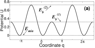
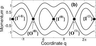
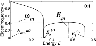
Figure 7: The potential $U(q)$, the separatrices in the phase space, and the eigenfrequency $\omega(E)$ for the unperturbed system (84) with $\Phi=0.2$, in (a), (b) and (c) respectively.

We now consider the addition of a time-periodic perturbation: as an example, we use an AC drive, which corresponds to a dipole Zaslavsky:1991 ; Landau:76 perturbation of the Hamiltonian:

$$\dot{q}=\partial H/\partial p,\quad\quad\dot{p}=-\partial H/\partial q,$$ (85)

$$H(p,q)=H_{0}(p,q)-hq\cos(\omega_{f}t).$$

The conventional scenario for the onset of global chaos between the separatrices of the system (84)-(85) is illustrated by Fig. 8. The figure presents the evolution of the stroboscopic Poincaré section as $h$ grows while $\omega_{f}$ is fixed at an arbitrarily chosen value away from $\omega_{m}$ and its harmonics. At small $h$, there are two thin chaotic layers around the inner and outer separatrices of the unperturbed system. Unbounded chaotic transport takes place only in the outer chaotic layer i.e. in a narrow energy range. As $h$ grows, so also do the layers. At some critical value $h_{gc}\equiv h_{gc}(\omega_{f})$, the layers merge. This may be considered as the onset of global chaos: the whole range of energies between the barrier levels is involved, with unbounded chaotic transport. The states $\{I^{(l)}\}\equiv\{p=0,q=\pi/2+2\pi l\}$ and $\{O^{(l)}\}\equiv\{p=0,q=-\pi/2+2\pi l\}$ (where $l$ is any integer) in the Poincaré section are associated respectively with the inner and outer saddles of the unperturbed system, and necessarily belong to the inner and outer chaotic layers, respectively. Thus, the necessary and sufficient condition for global chaos onset may be formulated as the possibility for the system placed initially in the state $\{I^{(0)}\}$ to pass beyond the neighbourhood of the “outer” states, $\{O^{(0)}\}$ or $\{O^{(1)}\}$, i.e. for the coordinate $q$ to become $<-\pi/2$ or $>3\pi/2$ at sufficiently large times $t\gg 2\pi/\omega_{f}$.

t]

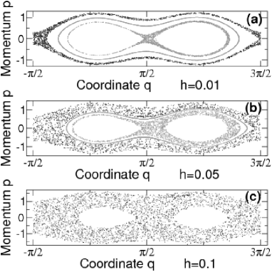
Figure 8: The evolution of the stroboscopic (at $t=n2\pi/\omega_{f}$ with $n=0,1,2,...$) Poincaré section of the system (84)-(85) with $\Phi=0.2$ as $h$ grows while $\omega_{f}=0.3$. The number of points in each trajectory is 2000. In (a) and (b), three characteristic trajectories are shown: the inner trajectory starts from the state $\{I^{(0)}\}\equiv\{p=0,q=\pi/2\}$ and is chaotic but bounded in space; the outer trajectory starts from $\{O^{(0)}\}\equiv\{p=0,q=-\pi/2\}$ and is chaotic and unbounded in coordinate; the third trajectory is an example of a regular trajectory separating the two chaotic ones. In (c), the chaotic trajectories mix.

A diagram in the $h-\omega_{f}$ plane, based on the above criterion, is shown in Fig. 9. The lower boundary of the shaded area represents the function $h_{gc}(\omega_{f})$. It has deep spikes i.e. cusp-like local minima. The most pronounced spikes are situated at frequencies $\omega_{f}=\omega_{s}^{(j)}$ that are slightly less than the odd multiples of $\omega_{m}$,

$$\omega_{s}^{(j)}\approx\omega_{m}(2j-1),\quad\quad j=1,2,...$$ (86)

The deepest minimum occurs at $\omega_{s}^{(1)}\approx\omega_{m}$: the value of $h_{gc}$ at the minimum, $h_{s}^{(1)}\equiv h_{gc}(\omega_{s}^{(1)})$, is approximately 40 times smaller than the value in the neighbouring pronounced local maximum of $h_{gc}(\omega_{f})$ at $\omega_{f}\approx 1$. As $n$ increases, the $n$th minimum becomes shallower. The function $h_{gc}(\omega_{f})$ is very sensitive to $\omega_{f}$ in the vicinity of the minima: for example, a reduction of $\omega_{f}$ from $\omega_{s}^{(1)}\approx 0.4$ of only 1% causes an increase in $h_{gc}$ of $\approx 30\%$.

t]

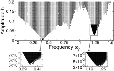
Figure 9: Diagram indicating the range of perturbation parameters (shaded) for which global chaos exists. The integration time for each point of the grid is $12000\pi$.

The origin of the spikes is related to the involvement of the resonance dynamics in separatrix chaos, similar to that considered in Sec. 3. In particular, the minima of the spikes correspond to the situation when the resonances almost touch, or slightly overlap with, the separatrices of the unperturbed system while overlapping each other. This is illustrated by the evolution of the Poincaré section as $h$ grows while $\omega_{f}\approx\omega_{s}^{(1)}$ (Fig. 10) and by its comparison with the corresponding evolution of resonance separatrices calculated in the resonance approximation (Fig. 11).

t]

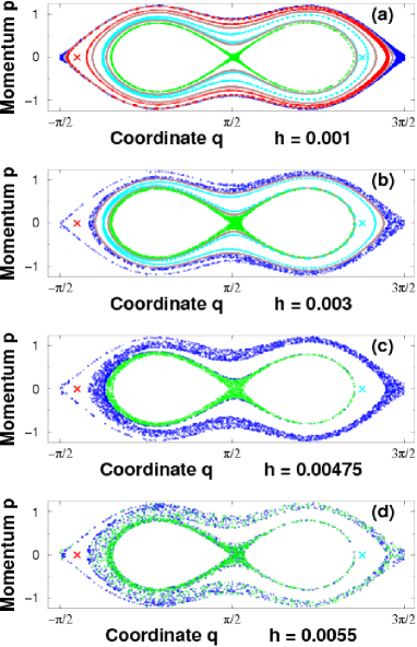
Figure 10: (Color version may be found in the online version of pre2008 as Fig. 5). The evolution of the stroboscopic Poincaré section of the system (84)-(85) with $\Phi=0.2$, as the amplitude $h$ of the perturbation grows, while the frequency remains fixed at $\omega_{f}=0.401$. The number of points in each trajectory is 2000. The chaotic trajectories starting from the states $\{I^{(0)}\}$ and $\{O^{(0)}\}$ are drawn in green and blue respectively. The stable stationary points of Eq. (98) for $n=1$ (i.e. for the 1st-order nonlinear resonances) are indicated by the red and cyan crosses. The chaotic layers associated with the resonances are indicated in red and cyan respectively, unless they merge with those associated with the green/blue chaotic trajectories. Examples of regular trajectories embracing the state $\{I^{(0)}\}$ while separating various chaotic trajectories are shown in brown.

b]

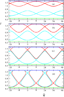
Figure 11: (Color version may be found in the online version of pre2008 as Fig. 6). The evolution of the separatrices of the 1st-order resonances within the resonance approximation (described by (16) with $n=1$) in the plane of action $I$ and slow angle $\tilde{\psi}$, for the same parameters as in Fig. 10 (boxes (a), (b), (c), (d) correspond to those in Fig. 10). Horizontal levels mark the values of $I$ corresponding to the barriers.

Sec. 4.1 below presents the self-consistent asymptotic theory of the minima of the spikes, based on an accurate analysis of the overlap of resonances with each other and on the matching between the separatrix map and the resonance Hamiltoinian (details of the matching are developed in Appendix). Sec. 4.2 presents the theory of the wings of the spikes Generalizations and applications are discussed in Sec. 4.3.

4.1 Asymptotic Theory For The Minima Of The Spikes

The eigenfrequency $\omega(E)$ stays close to its local maximum $\omega_{m}$ for most of the relevant range $[E_{b}^{(1)},E_{b}^{(2)}]$ (Fig. 7(c)). As shown below, $\omega(E)$ approaches a rectangular form in the asymptotic limit $\Phi\rightarrow 0$. Hence, if the perturbation frequency $\omega_{f}$ is close to $\omega_{m}$ or its odd multiples, $|\omega_{f}-(2j-1)\omega_{m}|\ll\omega_{m}$, then the energy widths of nonlinear resonances become comparable to the width of the whole range between the barriers (i.e. $E_{b}^{(2)}-E_{b}^{(1)}\approx 2\Phi$) at a rather small perturbation magnitude $h\ll\Phi$. Note that $\Phi$ determines the characteristic magnitude of the perturbation required for the conventional overlap of the separatrix chaotic layers, when $\omega_{f}$ is not close to any odd multiple of $\omega_{m}$ (Fig. 8 (c)). Thus, if $\omega_{f}\approx\omega_{s}^{(j)}$, the nonlinear resonances should play a crucial role in the onset of global chaos (cf. Fig. 10).

We note that it is not entirely obvious a priori whether it is indeed possible to calculate $h_{s}^{(j)}\equiv h_{gc}(\omega_{s}^{(j)})$ within the resonance approximation: in fact, it is essential for the separatrices of the nonlinear resonances to nearly touch the barrier levels, but the resonance approximation is invalid in the close vicinity of the barriers; furthermore, numerical calculations of resonances show that, if $\omega_{f}\approx\omega_{s}^{(j)}$, the perturbation amplitude $h$ at which the resonance separatrix touches a given energy level in the close vicinity of the barriers is very sensitive to $\omega_{f}$, apparently making the calculation of $h_{s}^{(j)}$ within the resonance approximation even more difficult.

Nevertheless, we show below in a self-consistent manner that, in the asymptotic limit $\Phi\rightarrow 0$, the relevant boundaries of the chaotic layers lie in the range of energies $E$ where $\omega(E)\approx\omega_{m}$. Therefore, the resonant approximation is valid and it allows us to obtain explicit asymptotic expressions both for $\omega_{s}^{(j)}$ and $h_{s}^{(j)}$, and for the wings of the spikes in the vicinities of $\omega_{s}^{(j)}$.

The asymptotic limit $\Phi\rightarrow 0$ is the most interesting one from a theoretical point of view because it leads to the strongest facilitation of the onset of global chaos, and it is most accurately described by the self-contained theory. Most of the theory presented below assumes this limit and concentrates therefore on the results to the lowest (i.e. leading) order in the small parameter.

On the applications side, the range of moderately small $\Phi$ is more interesting, since the chaos facilitation is still pronounced (and still described by the asymptotic theory) while the area of chaos between the separatrices is not too small (comparable with the area inside the inner separatrix): cf. Figs. 7, 8 and 10. To increase the accuracy of the theoretical description in this range, we estimate the next-order corrections and develop an efficient numerical procedure allowing for further corrections.

Resonant Hamiltonian and related quantities

Let $\omega_{f}$ be close to the $n$th odd harmonic of $\omega_{m}$, $n\equiv(2j-1)$. Over most of the range $[E_{b}^{(1)},E_{b}^{(2)}]$, except in the close vicinities of $E_{b}^{(1)}$ and $E_{b}^{(2)}$, the $n$th harmonic of the eigenoscillation is nearly resonant with the perturbation. Due to this, the (slow) dynamics of the action $I\equiv I(E)=(2\pi)^{-1}\oint dqp$ and the angle $\psi$ Chirikov:79 ; lichtenberg_lieberman ; Zaslavsky:1991 ; zaslavsky:1998 ; zaslavsky:2005 ; PR ; Landau:76 can be described by means of a resonance Hamiltonian similar in form to (16). The lower integration limit in the expression for $\tilde{H}$ may be chosen arbitrarily, and it will be convenient for us to use presently $I(E_{m})$ (instead of $I(E_{s})$ in (16)) where $E_{m}$ is the energy of the local maximum of $\omega(E)$ (Fig. 7(c)). To avoid confusion, we write the resonance Hamiltonian explicitly below after making this change:

$$\tilde{H}(I,\tilde{\psi})=\int_{I(E_{m})}^{I}{\rm d}\tilde{I}\;(n\omega-\omega_{f})\;-\;nhq_{n}\cos(\tilde{\psi})$$ (87)

$$\quad\;\equiv\;n(E-E_{m})-\omega_{f}(I-I(E_{m}))\;-\;nhq_{n}\cos(\tilde{\psi})\;,$$

$$I\equiv I(E)=\int_{E_{\rm min}}^{E}\frac{{\rm d}\tilde{E}}{\omega(\tilde{E})},\quad\quad E\equiv H_{0}(p,q),$$

$$\tilde{\psi}=n\psi-\omega_{f}t,\quad\quad$$

$$\psi=\pi+{\rm sign}(p)\omega(E)\int^{q}_{q_{\rm min}(E)}\frac{{\rm d}\tilde{q}}{\sqrt{2(E-U(\tilde{q}))}}+2\pi l,$$

$$q_{n}\equiv q_{n}(E)=\frac{2}{\pi}\int_{0}^{\pi/2}\!\!\!\!\!{\rm d}\psi\;q(E,\psi)\cos(n\psi),$$

$$|n\omega-\omega_{f}|\ll\omega,\quad\quad n\equiv 2j-1,\quad\quad j=1,2,3,\ldots$$

Let us derive explicit expressions for various quantities in (87). In the unperturbed case ($h=0$), the equations of motion (85) with $H_{0}$ (84) can be integrated oleg99 (see also Eq. (144) below), so that we can find $\omega(E)$:

$$\omega(E)=\frac{\pi(2E)^{1/4}}{2K\left[k\right]},\quad\quad k=\frac{1}{2}\sqrt{\frac{(\sqrt{2E}+1)^{2}-\Phi^{2}}{\sqrt{2E}}}\,,$$ (88)

where

$$K[k]=\int_{0}^{\frac{\pi}{2}}\frac{{\rm d}\phi}{\sqrt{1-k^{2}\sin^{2}(\phi)}},$$

is the complete elliptic integral of first order Abramovitz_Stegun . Using its asymptotic expression,

$$K[k\rightarrow 1]\simeq\frac{1}{2}\ln\left({16\over 1-k^{2}}\right),$$

we derive $\omega(E)$ in the asymptotic limit $\Phi\rightarrow 0$:

$$\omega(E)\simeq\frac{\pi}{\ln\left(\frac{64}{(\Phi-\Delta E)(\Phi+\Delta E)}\right)},$$ (89)

$$\Delta E\equiv E-\frac{1}{2},\quad\quad|\Delta E|<\Phi,\quad\quad\Phi\rightarrow 0.$$

As mentioned above,the function $\omega(E)$ (89) remains close to its maximum

$$\omega_{m}\equiv\max_{[E_{b}^{(1)},E_{b}^{(2)}]}\{\omega(E)\}\simeq\frac{\pi}{2\ln(8/\Phi)}\,$$ (90)

for most of the interbarrier range of energies $[1/2-\Phi,1/2+\Phi]$ (note that $E_{b}^{(1,2)}\approx 1/2\mp\Phi$ to first order in $\Phi$.); on the other hand, in the close vicinity of the barriers, where either $|\ln(1/(1-\Delta E/\Phi))|$ or $|\ln(1/(1+\Delta E/\Phi))|$ become comparable with, or larger than, $\ln(8/\Phi)$, $\omega(E)$ decreases rapidly to zero as $|\Delta E|\rightarrow\Phi$. The range where this takes place is $\sim\Phi^{2}$, and its ratio to the whole interbarrier range, $2\Phi$, is $\sim\Phi$ i.e. it goes to zero in the asymptotic limit $\Phi\rightarrow 0$: in other words, $\omega(E)$ approaches a rectangular form. As it will be clear from the following, it is this almost rectangular form of $\omega(E)$ which determines many of the characteristic features of the global chaos onset in systems with two or more separatrices.

One more quantity which strongly affects $(\omega_{s},h_{s})$ is the Fourier harmonic $q_{n}\equiv q_{n}(E)$. The system stays most of the time very close to one of the barriers. Consider the motion within one of the periods of the potential $U(q)$, between neighboring upper barriers $[q_{ub}^{(1)},q_{ub}^{(2)}]$ where $q_{ub}^{(2)}\equiv q_{ub}^{(1)}+2\pi$. If the energy $E\equiv 1/2+\Delta E$ lies in the relevant range $[E_{b}^{(1)},E_{b}^{(2)}]$, then the system will stay close to the lower barrier $q_{lb}\equiv q_{ub}^{(1)}+\pi$ for a time

$$T_{l}\approx 2\ln\left(\frac{1}{\Phi+\Delta E}\right)$$ (91)

during each period of eigenoscillation, while it will stay close to one of the upper barriers $q_{ub}^{(1,2)}\equiv q_{lb}\pm\pi$ for most of the remainder of the eigenoscillation,

$$T_{u}\approx 2\ln\left(\frac{1}{\Phi-\Delta E}\right)\quad.$$ (92)

Hence, the function $q(E,\psi)-q_{lb}$ may be approximated by the following piecewise even periodic function:

$$q(E,\psi)-q_{lb}=\left\{{}_{0\quad{\rm at}\quad\psi\in\left.\right]\frac{\pi}{2}\frac{T_{u}}{T_{l}+T_{u}},\pi-\frac{\pi}{2}\frac{T_{u}}{T_{l}+T_{u}}\left[\right.,}^{\pi\quad{\rm at}\quad\psi\in\left[0,\frac{\pi}{2}\frac{T_{u}}{T_{l}+T_{u}}\right]\cup\left[\pi-\frac{\pi}{2}\frac{T_{u}}{T_{l}+T_{u}},\pi\right],}\right.$$ (93)

$$q(E,-\psi)-q_{lb}=q(E,\psi)-q_{lb},\quad\quad q(E,\psi\pm 2\pi i)=q(E,\psi),\quad\quad i=1,2,3,...$$

Substituting the above approximation for $q(E,\psi)$ into the definition of $q_{n}$ (87), one can obtain:

$$q_{2j-1}\equiv q_{2j-1}(E)=\frac{2}{2j-1}\sin\left(\frac{(2j-1)\pi/2}{1+\frac{\ln\left(\frac{1}{\Phi+\Delta E}\right)}{\ln\left(\frac{1}{\Phi-\Delta E}\right)}}\right)\;,$$ (94)

$$\Phi\rightarrow 0,\quad\quad q_{2j}=0,\quad\quad j=1,2,3,...$$

At barrier energies, $q_{2j-1}$ takes the values

$$q_{2j-1}(E_{b}^{(1)})=0,\quad\quad q_{2j-1}(E_{b}^{(2)})=-(-1)^{j}{2\over(2j-1)}\,.$$ (95)

As $E$ varies in between its values at the barriers, $q_{2j-1}$ varies monotonically if $j=1$ and non-monotonically otherwise (cf. Fig. 16). But in any case, the significant variations occur mostly in the close vicinity of the barrier energies $E_{b}^{(1)}$ and $E_{b}^{(2)}$ while, for most of the range $[E_{b}^{(1)},E_{b}^{(2)}]$, the argument of the sine in Eq. (94) is close to $\,\pi/4$ and $\,q_{2j-1}$ is then almost constant:

$$q_{2j-1}\approx(-1)^{\left[\frac{2j-1}{4}\right]}\frac{\sqrt{2}}{2j-1},\quad\ j=1,2,3,\,\ldots,$$ (96)

$$\left|\ln\left(\frac{1+\Delta E/\Phi}{1-\Delta E/\Phi}\right)\right|\ll 2\ln\left(\frac{1}{\Phi}\right),$$

where $[\ldots]$ means the integer part.

In the asymptotic limit $\Phi\rightarrow 0$, the range of $\Delta E$ for which the approximate equality (96) for $q_{2j-1}$ is valid approaches the whole range $]-\Phi,\Phi[$.

We emphasize that $|q_{n}|$ determines the “strength” of the nonlinear resonances: therefore, apart from the nearly rectangular form of $\omega(E)$, the non-smallness of $|q_{n}|$ is an important additional factor strongly facilitating the onset of global chaos.

We shall need also an asymptotic expression for the action $I$. Substituting $\omega(E)$ (89) into the definition of $I(E)$ (87) and carrying out the integration, we obtain

$$I(E)=I(1/2)+\frac{\Delta E\ln\left(\frac{64{\rm e}^{2}}{\Phi^{2}-(\Delta E)^{2}}\right)+\Phi\ln\left(\frac{\Phi-\Delta E}{\Phi+\Delta E}\right)}{\pi}\;,\quad\quad\Phi\rightarrow 0.$$ (97)

Reconnection of resonance separatrices

We now turn to analysis of the phase space of the resonance Hamiltonian (87). The evolution of the Poincaré section (Fig. 10) suggests that we need to find a separatrix of (87) that undergoes the following evolution as $h$ grows: for sufficiently small $h$, the separatrix does not overlap chaotic layers associated with the barriers while, for $h>h_{gc}(\omega_{f})$, it does overlap them. The relevance of such a condition will be further justified.

Consider $\omega_{f}\approx n\omega_{m}$ with a given odd $n$. For the sake of convenience, let us write down the equations of motion (87) explicitly:

$$\dot{I}=-\frac{\partial\tilde{H}}{\partial\tilde{\psi}}\equiv-nhq_{n}\sin(\tilde{\psi}),\quad\quad\dot{\tilde{\psi}}=\frac{\partial\tilde{H}}{\partial I}\equiv n\omega-\omega_{f}-nh\frac{{\rm d}q_{n}}{{\rm d}I}\cos(\tilde{\psi}).$$ (98)

Any separatrix necessarily includes one or more unstable stationary points. The system of dynamic equations (98) may have several stationary points per $2\pi$ interval of $\tilde{\psi}$. Let us first exclude those points which are irrelevant to a separatrix undergoing the evolution described above.

Given that $q_{n}(E_{b}^{(1)})=0$, there are two unstable stationary points with $I$ corresponding to $E=E_{b}^{(1)}$ and $\tilde{\psi}=\pm\pi/2$. They are irrelevant because, even for an infinitely small $h$, each of them necessarily lies inside the corresponding barrier chaotic layer.

If $E\neq E_{b}^{(1)}$, then $q_{n}\neq 0$, so $\dot{I}=0$ only if $\tilde{\psi}$ is equal either to 0 or to $\pi$. Substituting these values into the second equation of (98) and putting $\dot{\tilde{\psi}}=0$, we obtain the equations for the corresponding actions:

$$X_{\mp}(I)\equiv n\omega-\omega_{f}\mp nh{\rm d}q_{n}/{\rm d}I=0,$$ (99)

where the signs “-” and “+” correspond to $\tilde{\psi}=0$ and $\tilde{\psi}=\pi$ respectively. A typical example of the graphical solution of equations (99) for $n=1$ is shown in Fig. 12. Two of the roots corresponding to $\tilde{\psi}=\pi$ are very close to the barrier values of $I$ (recall that the relevant values of $h$ are small). These roots arise due to the divergence of ${\rm d}q/{\rm d}I$ as $I$ approaches any of the barrier values. The lower/upper root corresponds to a stable/unstable point, respectively. However, for any $n$, both these points and the separatrix generated by the unstable point necessarily lie in the ranges covered by the barrier chaotic layers. Therefore, they are also irrelevant. For $n>1$, the number of roots of (99) in the vicinity of the barriers may be larger (due to oscillations of the modulus and sign of ${\rm d}q_{n}/{\rm d}I$ in the vicinity of the barriers) but they all are irrelevant for the same reason, at least to leading-order terms in the expressions for the spikes’ minima.

t]

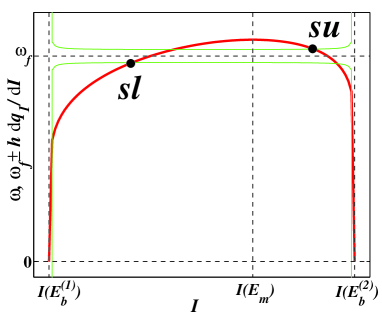
Figure 12: (Color version may be found in the online version of pre2008 as Fig. 7). A schematic example illustrating the graphical solutions of Eqs. (99) for $n=1$, as intersections of the curve $\omega(I)$ (thick solid red line) with the curves $\omega_{f}\pm h{\rm d}q_{n}(I)/{\rm d}I$ (thin solid green lines). The solutions corresponding to the lower and upper relevant saddles (defined by Eq. (100)) are marked by dots and by the labels $sl$ and $su$ respectively (we do not mark other solutions because they are irrelevant).

Consider the stationary points corresponding to the remaining four roots of equations (99). Just these points are conventionally associated with nonlinear resonances Chirikov:79 ; lichtenberg_lieberman ; Zaslavsky:1991 ; zaslavsky:1998 ; zaslavsky:2005 ; PR . It follows from the analysis of equations (98) linearized near the stationary points (cf. Chirikov:79 ; lichtenberg_lieberman ; Zaslavsky:1991 ; zaslavsky:1998 ; zaslavsky:2005 ; PR ), two of them are stable (elliptic) points, while two others are unstable (hyperbolic) points, often called saddles. These saddles are of central interest in the context of our work. They belong to the separatrices dividing the $I-\tilde{\psi}$ plane for regions with topologically different trajectories.

We shall identify the relevant saddles as those with the lower action/energy (using the subscript “$sl$”) and upper action/energy (using the subscript “$su$”). The positions of the saddles in the $I-\tilde{\psi}$ plane are defined by the following equations (cf. Figs. 11 and 12):

$$g\equiv{\rm sgn}(q_{n}(I_{su,sl}))={\rm sgn}\left((-1)^{\left[\frac{n}{4}\right]}\right),$$ (100)

$$\tilde{\psi}_{sl}=\pi(1+g)/2,\quad\quad\tilde{\psi}_{su}=\pi(1-g)/2,$$

$$X_{g}(I_{sl})=X_{-g}(I_{su})=0,\quad\quad\frac{{\rm d}X_{g}(I_{sl})}{{\rm d}I_{sl}}>0,\quad\quad\frac{{\rm d}X_{-g}(I_{su})}{{\rm d}I_{su}}<0,$$

where $[...]$ means an integer part, $X_{\pm}(I)$ are defined in Eq. (99) while $I_{sl}$ and $I_{su}$ are closer to $I(E_{m})$ than any other solution of (100) (if any) from below and from above, respectively.

Given that the values of $h$ relevant to the minima of the spikes asymptotically approach 0 in the asymptotic limit $\Phi\rightarrow 0$, one may neglect the last term in the definition of $X_{\mp}$ in Eq. (99) in the lowest-order approximation, so that the equations $X_{\mp}=0$ reduce to the simplified resonance condition

$$n\omega(I_{su,sl})=\omega_{f}.$$ (101)

Substituting here Eq. (89) for $\omega$, we obtain explicit expressions for the energies in the saddles:

$$E_{su,sl}\approx\frac{1}{2}\pm\Delta E^{(1)},$$ (102)

$$\Delta E^{(1)}\equiv\sqrt{\Phi^{2}-64\exp\left(-\frac{n\pi}{\omega_{f}}\right)},\quad\quad\omega_{f}\leq n\omega_{m}.$$

The corresponding actions $I_{su,sl}$ are expressed via $E_{su,sl}$ by means of Eq. (97).

For $\omega_{f}\approx n\omega_{m}$, the values of $E_{su,sl}$ (102) lie in the range where the expression (96) for $q_{n}$ holds true. This will be confirmed by the results of calculations based on this assumption.

Using (100) for the angles and (102) for the energies, and the asymptotic expressions (89), (96) and (97) for $\omega(E)$, $q_{n}(E)$ and $I(E)$ respectively, and allowing for the resonance condition (101), we obtain explicit expressions for the values of the Hamiltonian (87) at the saddles:

$$\tilde{H}_{sl}=-\tilde{H}_{su}=\frac{\omega_{f}}{\pi}\left[2\Delta E^{(1)}-\Phi\ln\left(\frac{\Phi+\Delta E^{(1)}}{\Phi-\Delta E^{(1)}}\right)\right]+h\sqrt{2}.$$ (103)

As the analysis of simulations suggests and as it is self-consistently shown further, one of the main conditions which should be satisfied in the spikes is the overlap in phase space between the separatrices of the nonlinear resonances, which is known as separatrix reconnection PR ; Howard:84 ; Howard:95 ; Diego ; James ; Albert . Given that the Hamiltonian $\tilde{H}$ is constant along any trajectory of the system (87), the values of $\tilde{H}$ in the lower and upper saddles of the reconnected separatrices are equal to each other:

$$\tilde{H}_{sl}=\tilde{H}_{su}\,.$$ (104)

This may be considered as the necessary and sufficient condition for the reconnection. Taking into account that $\tilde{H}_{sl}=-\tilde{H}_{su}$ (see (103)), it follows from (104) that

$$\tilde{H}_{sl}=\tilde{H}_{su}=0.$$ (105)

Explicitly, the relations in (105) reduce to

$$h\equiv h(\omega_{f})=\frac{\omega_{f}}{\sqrt{2}\pi}\left[\Phi\ln\left(\frac{\Phi+\Delta E^{(1)}}{\Phi-\Delta E^{(1)}}\right)-2\Delta E^{(1)}\right],$$ (106)

$$\Delta E^{(1)}\equiv\sqrt{\Phi^{2}-64\exp(-\frac{n\pi}{\omega_{f}})},\quad\quad 0<\omega_{m}-\omega_{f}/n\ll\omega_{m}\equiv\frac{\pi}{2\ln(8/\Phi)},$$

$$n=1,3,5,...$$

The function $h(\omega_{f})$ (106) decreases monotonically to zero as $\omega_{f}$ grows from $0$ to $n\omega_{m}$, where the line abruptly stops. Fig. 15 shows the portions of the lines (106) relevant to the left wings of the 1st and 2nd spikes (for $\Phi=0.2$).

Barrier chaotic layers

The next step is to find the minimum value of $h$ for which the resonance separatrix overlaps the chaotic layer related to a potential barrier. With this aim, we study how the relevant outer boundary of the chaotic layer behaves as $h$ and $\omega_{f}$ vary. Assume that the relevant $\omega_{f}$ is close to $n\omega_{m}$ while the relevant $h$ is sufficiently large for $\omega(E)$ to be close to $\omega_{m}$ at all points of the outer boundary of the layer (the results will confirm these assumptions). Then the motion along the regular trajectory infinitesimally close to the layer boundary may be described within the resonance approximation (87). Hence the boundary may also be described as a trajectory of the resonant Hamiltonian (87). This is explicitly proved in the Appendix, using a separatrix map analysis allowing for the validity of the relation $\omega(E)\approx\omega_{m}$ for all $E$ relevant to the boundary of the chaotic layer. The main results are presented below. For the sake of clarity, we present them for each layer separately, although they are similar in practice.

4.1.3.1 Lower Layer

Let $\omega_{f}$ be close to any of the spikes’ minima.

One of the key roles in the formation of the upper boundary of the layer is played by the angle-dependent quantity $\delta_{l}|\sin(\tilde{\psi})|$ which we call the generalized separatrix split (GSS) for the lower layer, alluding to the conventional separatrix split zaslavsky:1998 for the lower layer $\delta_{l}\equiv|\epsilon^{(low)}(\omega_{f})|h$ with $\epsilon^{(low)}$ given by Eq. (172) (cf. also (4)). Accordingly, we use the term “lower GSS curve” for the following curve in the $I-\tilde{\psi}$ plane:

$$I=I_{\rm GSS}^{(l)}(\tilde{\psi})\equiv I(E_{b}^{(1)}+\delta_{l}|\sin(\tilde{\psi})|).$$ (107)

4.1.3.1.1 Relatively Small Values Of $h$

If $h<h_{cr}^{(l)}(\omega_{f})$, where the critical value $\,h_{cr}^{(l)}(\omega_{f})\,$ is determined by Eq. (125) (its origin will be explained further), then there are differences in the boundary formation for the frequency ranges of odd and even spikes. We describe these ranges separately.

1. Odd spikes

In this case, the boundary is formed by the trajectory of the Hamiltonian (87) tangent to the GSS curve (see Fig. 22(a); cf. also Figs. 1(c), 13(a), 14(b), 14(c)). There are two tangencies in the angular range $]-\pi,\pi[$: they occur at the angles $\pm\tilde{\psi}_{t}^{(l)}$ where $\tilde{\psi}_{t}^{(l)}$ is determined by Eq. (182).

In the ranges of $h$ and $\omega_{f}$ relevant to the spike minimum, the asymptotic expressions for $\delta_{l}$ and $\tilde{\psi}_{t}^{(l)}$ are:

$$\delta_{l}=\sqrt{2}\pi h,$$ (108)

$$\tilde{\psi}_{t}^{(l)}=(-1)^{\left[\frac{n}{4}\right]}\sqrt{\frac{n\pi}{8\ln\left(1/\Phi\right)}}+\pi\frac{1-(-1)^{\left[\frac{n}{4}\right]}}{2}.$$ (109)

Hence, the asymptotic value for the deviation of the tangency energy $E_{t}^{(l)}$ from the lower barrier reduces to:

$$E_{t}^{(l)}-E_{b}^{(1)}\equiv\delta_{l}\sin(\tilde{\psi}_{t}^{(l)})=\frac{\pi^{3/2}}{2}\frac{h}{\sqrt{\ln\left(1/\Phi\right)/n}}.$$ (110)

The minimum energy on the boundary, $E_{\min}^{(l)}$, corresponds to $\tilde{\psi}=$ $0$ or $\pi$ for even or odd values of $[n/4]$ respectively. Thus, it can be found from the equality

$$\tilde{H}\left(I(E_{\min}^{(l)}),\tilde{\psi}=\pi(1-(-1)^{\left[\frac{n}{4}\right]})/2\right)=\tilde{H}\left(I_{t}^{(l)}\equiv I(E_{t}^{(l)}),\tilde{\psi}_{t}^{(l)}\right).$$ (111)

At $\Phi\rightarrow 0$, Eq. (111) yields the following expression for the minimal deviation of energy on the boundary from the barrier:

$$\delta_{\min}^{(l)}\equiv E_{\min}^{(l)}-E_{b}^{(1)}=(E_{t}^{(l)}-E_{b}^{(1)})/\sqrt{{\rm e}}=\frac{\pi^{3/2}}{2\sqrt{{\rm e}}}\frac{h}{\sqrt{\ln\left(1/\Phi\right)/n}}.$$ (112)

In the context of the onset of global chaos, the most important property of the boundary is that the maximum deviation of its energy from the barrier, $\delta_{\max}^{(l)}$, should greatly exceed both $\delta_{\min}^{(l)}$ and $\delta_{l}$. As $h\rightarrow h_{cr}^{(l)}$, the maximum of the boundary approaches the saddle “sl”.

2. Even spikes

In this case, the Hamiltonian (87) possesses saddles “s” in the close vicinity to the lower barrier (see Fig. 22(b)). Their angles differ by $\pi$ from those of “sl”:

$$\tilde{\psi}_{s}=\pi\frac{1-(-1)^{\left[\frac{n}{4}\right]}}{2}+2\pi m,\quad\quad m=0,\pm 1,\pm 2,\ldots,$$ (113)

while the deviation of their energies from the barrier still lies in the relevant (resonant) range and reads, in the lowest-order approximation,

$$\delta_{s}=\frac{\pi}{2\sqrt{2}}\frac{h}{\ln(\ln(1/\Phi))}.$$ (114)

The lower whiskers of the separatrix generated by these saddles intersect the GSS curve while the upper whiskers in the asymptotic limit do not intersect it (Fig. 22(b)). Thus, it is the upper whiskers of the separatrix which form the boundary of the chaotic layer in the asymptotic limit. The energy on the boundary takes the minimal value right on the saddle “s”, so that

$$\delta_{\min}^{(l)}=\delta_{s}=\frac{\pi}{2\sqrt{2}}\frac{h}{\ln(\ln(1/\Phi))}.$$ (115)

Similar to the case of the odd spikes, the maximal deviation of the energy from the barrier (measured along the boundary) greatly exceeds both $\delta_{\min}^{(l)}$ and $\delta_{l}$. As $h\rightarrow h_{cr}^{(l)}$, the maximum of the boundary approaches the saddle “sl”.

4.1.3.1.2 Relatively Large Values Of $h$

If $h>h_{cr}^{(l)}(\omega_{f})$, the previously described trajectory (either the tangent one or the separatrix, for the odd or even spike ranges respectively) is encompassed by the separatrix of the lower nonlinear resonance and typically forms the boundary of a major stability island inside the lower layer (reproduced periodically in $\tilde{\psi}$ with the period $2\pi$). The upper outer boundary of the layer is formed by the upper part of the resonance separatrix. This may be interpreted as the absorption of the lower resonance by the lower chaotic layer.

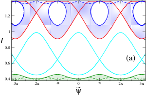
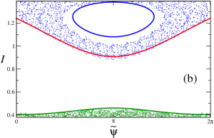
Figure 13: (Color version may be found in the online version of pre2008 as Fig. 8). (a) Chaotic layers (shaded in green and blue, for the upper and lower layers respectively) in the plane of action $I$ and slow angle $\tilde{\psi}$, as described by our theory. Parameters are the same as in Figs. 10(b) and 11(b). The lower and upper boundaries of the figure box coincide with $I(E_{b}^{(1)})$ and $I(E_{b}^{(2)})$ respectively. The resonance separatrices are drawn by the cyan and red solid lines (for the lower and upper resonances respectively). Dashed green and blue lines mark the curves $I=I_{\rm GSS}^{(l)}(\tilde{\psi})\equiv I(E=E_{b}^{(1)}+\delta_{l}|\sin(\tilde{\psi})|)$ and $I=I_{\rm GSS}^{(u)}(\tilde{\psi})\equiv I(E=E_{b}^{(2)}-\delta_{u}|\sin(\tilde{\psi})|)$ respectively, where $\delta_{l}$ and $\delta_{u}$ are the values of the separatrix split related to the lower and upper barrier respectively. The upper boundary of the lower layer is formed by the trajectory of the resonant Hamiltonian system (87) tangent to the curve $I=I_{\rm GSS}^{(l)}(\tilde{\psi})$. The lower boundary of the upper layer is formed by the lower part of the upper (red) resonance separatrix. The periodic closed loops (solid blue lines) are the trajectories of the system (87) tangent to the curve $I_{\rm GSS}^{(u)}(\tilde{\psi})$: they form the boundaries of the major stability islands inside the upper chaotic layer. (b) Comparison of the chaotic layers obtained from computer simulations (dots) with the theoretically calculated boundaries (solid lines) shown in the box (a).

4.1.3.2 Upper Layer

Let $\omega_{f}$ be close to any of the spikes’ minima.

One of the key roles in the formation of the lower boundary of the layer is played by the angle-dependent quantity $\delta_{u}|\sin(\tilde{\psi})|$ which we call the generalized separatrix split (GSS) for the upper layer; $\delta_{u}$ is the separatrix split for the upper layer: $\delta_{u}=|\epsilon^{(up)}(\omega_{f})|h$ with $\epsilon^{(up)}$ given by Eq. (204). Accordingly, we use the term “upper GSS curve” for the following curve in the $I-\tilde{\psi}$ plane:

$$I=I_{\rm GSS}^{(u)}(\tilde{\psi})\equiv I(E_{b}^{(2)}-\delta_{u}|\sin(\tilde{\psi})|).$$ (116)

4.1.3.2.1 Relatively Small Values Of $h$

If $h<h_{cr}^{(u)}(\omega_{f})$, where the critical value $\,h_{cr}^{(u)}(\omega_{f})\,$ is determined by Eq. (126) (its origin will be explained further), then there are some differences in the boundary formation in the frequency ranges of odd and even spikes: for odd spikes, the formation is similar to the one for even spikes in the lower-layer case and vice versa.

1. Odd spikes

In the case of odd spikes, the Hamiltonian (87) possesses saddles “$\tilde{s}$” in the close vicinity of the upper barrier, analogous to the saddles “s” near the lower barrier in the case of even spikes. Their angles are shifted by $\pi$ from those of “s”:

$$\tilde{\psi}_{\tilde{s}}=\tilde{\psi}_{s}+\pi=\pi\frac{1+(-1)^{\left[\frac{n}{4}\right]}}{2}+2\pi m,\quad\quad m=0,\pm 1,\pm 2,\ldots$$ (117)

The deviation of their energies from the upper barrier coincides, in the lowest-order approximation, with $\delta_{s}$:

$$\delta_{\tilde{s}}=\delta_{s}=\frac{\pi}{2\sqrt{2}}\frac{h}{\ln(\ln(1/\Phi))}.$$ (118)

The upper whiskers of the separatrix generated by these saddles intersect the upper GSS curve while the lower whiskers in the asymptotic limit do not intersect it. Thus, it is the lower whiskers of the separatrix which form the boundary of the chaotic layer in the asymptotic limit. The deviation of the energy from the upper barrier takes its minimal value (measured along the boundary) right on the saddle “$\tilde{s}$”,

$$\delta_{\min}^{(u)}=\delta_{\tilde{s}}=\frac{\pi}{2\sqrt{2}}\frac{h}{\ln(\ln(1/\Phi))}.$$ (119)

The maximal deviation of the energy from the barrier (along the boundary) greatly exceeds both $\delta_{\min}^{(u)}$ and $\delta_{u}$. As $h\rightarrow h_{cr}^{(u)}$, the maximum of the boundary approaches the saddle “su”.

2. Even spikes

The boundary is formed by the trajectory of the Hamiltonian (87) tangent to the GSS curve. There are two tangencies in the angle range $]-\pi,\pi[$: they occur at the angles $\pm\tilde{\psi}_{t}^{(u)}$ where $\tilde{\psi}_{t}^{(u)}$ is determined by Eq. (202).

In the ranges of $h$ and $\omega_{f}$ relevant to the spike minimum, the expressions for $\delta_{u}$ and $\tilde{\psi}_{t}^{(u)}$ in the asymptotic limit $\Phi\rightarrow 0$ are similar to the analogous quantities in the lower-layer case:

$$\delta_{u}=\sqrt{2}\pi h,$$ (120)

$$\tilde{\psi}_{t}^{(u)}=-(-1)^{\left[\frac{n}{4}\right]}\sqrt{\frac{n\pi}{8\ln\left(\frac{1}{\Phi}\right)}}+\pi\frac{1+(-1)^{\left[\frac{n}{4}\right]}}{2}.$$ (121)

Hence, the asymptotic value for the deviation of the tangency energy $E_{t}^{(u)}$ from the upper barrier reduces to:

$$E_{b}^{(2)}-E_{t}^{(u)}\delta_{u}\left|\pi\frac{1+(-1)^{\left[\frac{n}{4}\right]}}{2}-\tilde{\psi}_{t}^{(u)}\right|=\frac{\pi^{3/2}}{2}\frac{h}{\sqrt{\ln\left(1/\Phi\right)/n}}.$$ (122)

The maximal energy on the boundary, $E_{\max}^{(u)}$, corresponds to $\tilde{\psi}=\pi(1+(-1)^{[n/4]})/2$. Thus, it can be found from the equality

$$\tilde{H}(I=I(E_{\max}^{(u)}),\tilde{\psi}=\pi(1+(-1)^{[n/4]})/2)=\tilde{H}(I_{t}^{(u)}\equiv I(E_{t}^{(u)}),\tilde{\psi}_{t}^{(u)}).$$ (123)

At $\Phi\rightarrow 0$, Eq. (123) yields the following expression for the minimal deviation of energy from the barrier (measured along the boundary):

$$\delta_{\min}^{(u)}\equiv E_{b}^{(2)}-E_{\max}^{(u)}=(E_{b}^{(2)}-E_{t}^{(u)})/\sqrt{{\rm e}}=\frac{\pi^{3/2}}{2{\rm e}^{1/2}}\frac{h}{\sqrt{\ln\left(1/\Phi\right)/n}}.$$ (124)

4.1.3.2.2 Relatively Large Values Of $h$

If $h>h_{cr}^{(u)}(\omega_{f})$ (cf. Fig. 13(a)), the previously described trajectory (either the tangent one or the separatrix, for the even and odd spikes ranges respectively) is encompassed by the separatrix of the upper nonlinear resonance and typically forms the boundary of a major stability island inside the upper layer (reproduced periodically in $\tilde{\psi}$ with the period $2\pi$). The lower outer boundary of the layer is formed in this case by the lower part of the resonance separatrix. This may be interpreted as the absorption of the upper resonance by the upper chaotic layer.

The self-consistent description of chaotic layers given above, and in more detail in the Appendix, is the first main result of this section. It provides a rigorous basis for our intuitive assumption that the minimal value of $h$ at which the layers overlap corresponds to the reconnection of the nonlinear resonances with each other while the reconnected resonances touch one of the layers and also touch/overlap another layer. It is gratifying that we have obtained a quantitative theoretical description of the chaotic layer boundaries in the phase space, including even the major stability islands, that agrees well with the results of simulations (see Fig. 13(b)). To the best of our knowledge it was the first ever pre2008 quantitative description of the layer boundaries in the phase space.

Onset of global chaos: the spikes’ minima

The condition for the merger of the lower resonance and the lower chaotic layer may be written as

$$\tilde{H}(I=I(E=E_{b}^{(1)}+\delta^{(l)}_{\min}),\tilde{\psi}=\pi(1-(-1)^{[n/4]})/2)=\tilde{H}_{sl}.$$ (125)

The condition for the merger of the upper resonance and the upper chaotic layer may be written as

$$\tilde{H}(I=I(E=E_{b}^{(2)}-\delta^{(u)}_{\min}),\tilde{\psi}=\pi(1+(-1)^{[n/4]})/2)=\tilde{H}_{su}.$$ (126)

For the onset of global chaos related to the spike minimum, either of Eqs. (125) and (126) should be combined with the condition of the separatrix reconnection (104). Let us seek first only the leading terms of $h_{s}\equiv h_{s}(\Phi)$ and $\omega_{s}\equiv\omega_{s}(\Phi)$. Then (104) may be replaced by its lowest-order approximation (105) or, equivalently, (106). Using also the lowest-order approximation for the barriers ($E_{b}^{(1,2)}\approx 1/2\mp\Phi$), we reduce Eqs. (125), (126) respectively to

$$\tilde{H}(I=I(E=1/2-\Phi+\delta^{(l)}_{\min}),\tilde{\psi}=\pi(1-(-1)^{[n/4]})/2)=0,$$ (127)

$$\tilde{H}(I=I(E=1/2+\Phi-\delta^{(u)}_{\min}),\tilde{\psi}=\pi(1+(-1)^{[n/4]})/2)=0,$$ (128)

where $\delta^{(l)}_{\min}$ is given by (112) or (115) for the odd or even spikes respectively, while $\delta^{(u)}_{\min}$ is given by (119) or (124) for the odd or even spikes respectively.

To the leading order, the solution $(h_{s}^{(l)},\omega_{s}^{(l)})$ of the system of equations (106),(127) and the solution $(h_{s}^{(u)},\omega_{s}^{(u)})$ of the system of equations (106),(128) turn out identical. For the sake of brevity, we derive below just $(h_{s}^{(l)},\omega_{s}^{(l)})$, denoting the latter, in short, as $(h_{s},\omega_{s})$.

The system of algebraic equations (106) and (127) is still too complicated for us to find its exact solution. However, we need only the lowest-order solution – and this simplifies the problem. Still, even this simplified problem is not trivial, both because the function $h_{s}(\Phi)$ turns out to be non-analytic and because $\Delta E^{(1)}$ in (106) is very sensitive to $\omega_{f}$ in the relevant range. Despite these difficulties, we have found the solution in a self-consistent way, as briefly described below.

Assume that the asymptotic dependence $h_{s}(\Phi)$ is:

$$h_{s}=a\frac{\Phi}{\ln(4{\rm e}/\Phi)}\,,$$ (129)

where the constant $a$ may be found from the asymptotic solution of (106), (127), (129).

Substituting the energies $E=1/2-\Phi+\delta^{(l)}_{\min}$ and $E=1/2+\Phi-\delta^{(u)}_{\max}$ in (89) and taking account of (112), (115), (119), (124) and (129), we find that, both for the odd and even spikes, the inequality

$$\omega_{m}-\omega(E)\ll\omega_{m}$$ (130)

holds over the whole relevant range of energies, i.e. for

$$\Delta E\in[-\Phi+\delta^{(l)}_{\min},\Phi-\delta^{(u)}_{\min}].$$ (131)

Thus, the resonant approximation is valid over the whole range (131). Eq. (96) for $q_{n}(E)$ is valid over the whole relevant range of energies too.

Consider Eq. (127) in an explicit form. Namely, we express $\omega_{f}$ from (127), using Eqs. (87), (96), and (97), using also (112) or (115) for odd or even spikes and (129):

$$\omega_{f}=\frac{n\pi}{2\ln\left(\frac{4{\rm e}}{\Phi}\right)}\left\{1+\frac{h\sqrt{2}}{n\Phi}+O\left(\frac{1}{\ln^{2}(4{\rm e}/\Phi)}\right)\right\}.$$ (132)

We emphasize that the value of $\delta_{\min}^{(l)}$ enters explicitly only the term $O(\ldots)$ while, as is clear from the consideration below, this term does not affect the leading terms in $(h_{s},\omega_{s})$. Thus, $\delta_{\min}^{(l)}$ does not affect the leading term of $\omega_{s}$ at all, while it affects the leading term of $h_{s}$ only implicitly: $\delta_{\min}^{(l)}$ lies in the range of energies where $nq_{n}(E)\approx\sqrt{2}$. This latter quantity is present in the second term in the curly brackets in (132) and, as becomes clear from further consideration, $h_{s}$ is proportional to it.

Substituting (132) into the expression for $\Delta E^{(1)}$ in (106), using (129) and keeping only the leading terms, we obtain

$$\Delta E^{(1)}=\Phi\sqrt{1-4{\rm e}^{c-2}},\quad\quad c\equiv\frac{2\sqrt{2}}{n}a.$$ (133)

Substituting $\Delta E^{(1)}$ from (133) into Eq. (106) for $h(\omega_{f})$ and allowing for (129) once again, we arrive at a transcendental equation for $c$:

$$\ln\left(\frac{1+\chi(c)}{1-\chi(c)}\right)-2\chi(c)=c,\quad\quad\chi(c)\equiv\sqrt{1-4{\rm e}^{c-2}}.$$ (134)

An approximate numerical solution of Eq. (134) is:

$$c\simeq 0.179.$$ (135)

Thus, the final leading-order asymptotic formulæ for $\omega_{f}$ and $h$ in the minima of the spikes are the following:

$$\omega_{s0}\equiv\omega_{s0}^{\left(\frac{n+1}{2}\right)}=n\frac{\pi}{2\ln\left(\frac{4{\rm e}}{\Phi}\right)},\quad\quad h_{s0}\equiv h_{s0}^{\left(\frac{n+1}{2}\right)}=n\frac{c}{2\sqrt{2}}\frac{\Phi}{\ln\left(\frac{4{\rm e}}{\Phi}\right)},$$ (136)

$$n=1,3,5,...,\quad\quad\Phi\rightarrow 0,$$

where the constant $c\simeq 0.179$ is the solution of Eq. (134).

The self-consistent derivation of the explicit asymptotic formulæ for the minima of $h_{gc}(\omega_{f})$ constitutes the second main result of this section. These formulæ allow one to predict immediately the parameters for the weakest perturbation that may lead to global chaos.

Numerical example and next-order corrections

For $\Phi=0.2$, the numerical simulations give the following values for the frequencies at the minima of the first two spikes (see Fig. 9):

$$\omega_{s}^{(1)}\approx 0.4005\pm 0.0005,\quad\quad\omega_{s}^{(2)}\approx 1.24\pm 0.005.$$ (137)

By the lowest-order formula (136), the values are:

$$\omega_{s0}^{(1)}\approx 0.393,\quad\quad\omega_{s0}^{(2)}\approx 1.18,$$ (138)

in rather good agreement with the simulations.

The next-order correction for $\omega_{s}$ can immediately be found from Eq. (132) for $\omega_{f}$ and from Eq. (136) for $h_{s0}$, so that

$$\omega_{s1}\simeq\omega_{s0}(1+\frac{c}{2\ln\left(\frac{4{\rm e}}{\Phi}\right)})\approx\frac{n\pi\left(1+\frac{0.09}{\ln\left(\frac{4{\rm e}}{\Phi}\right)}\right)}{2\ln\left(\frac{4{\rm e}}{\Phi}\right)}\,,\quad\quad n=1,3,5,...$$ (139)

The formula (139) agrees with the simulations even better than the lowest-order approximation:

$$\omega_{s1}^{(1)}\approx 0.402,\quad\quad\omega_{s1}^{(2)}\approx 1.21.$$ (140)

For $h$ in the spikes minima, the simulations give the following values (see Fig. 9):

$$h_{s}^{(1)}\approx 0.0049,\quad\quad h_{s}^{(2)}\approx 0.03.$$ (141)

The values according to the lowest-order formula (52) are:

$$h_{s0}^{(1)}\approx 0.0032,\quad\quad h_{s0}^{(2)}\approx 0.01.$$ (142)

The theoretical value $h_{s0}^{(1)}$ gives reasonable agreement with the simulation value $h_{s}^{(1)}$. The theoretical value $h_{s0}^{(2)}$ gives the correct order of magnitude for the simulation value $h_{s}^{(2)}$. Thus, the accuracy of the lowest-order formula (136) for $h_{s}$ is much lower than that for $\omega_{s}$: this is due to the steepness of $h_{gc}(\omega_{f})$ in the ranges of the spikes (the steepness, in turn, is due to the flatness of the function $\omega(E)$ near its maximum). Moreover, as the number of the spike $j$ increases, the accuracy of the lowest-order value $h_{s0}^{(j)}$ significantly decreases. The latter can be explained as follows. For the next-order correction to $h_{s0}^{(j)}$, the dependence on $\Phi$ reads as:

$$\frac{h_{s1}^{(j)}-h_{s0}^{(j)}}{h_{s0}^{(j)}}\propto\frac{1}{\ln(4{\rm e}/\Phi)}.$$ (143)

At least some of the terms in this correction are positive and proportional to $h_{s0}^{(j)}$ (e.g. due to the difference between the exact equation (99) and its approximate version (101)), while $h_{s0}^{(j)}$ is proportional to $n\equiv 2j-1$. Thus, for $\Phi=0.2$, the relative correction for the 1st spike is $\sim 0.25$ while the correction for the 2nd spike is a few times larger i.e. $\sim 1$. But the latter means that, for $\Phi=0.2$, the asymptotic theory for the 2nd spike cannot pretend to be a quantitative description of $h_{s}^{(2)}$, but only provides the correct order of magnitude. Besides, if $n>1$ while $\Phi$ exceeds some critical value, then the search of the minimum involves Eq. (150) rather than Eq. (104), as explained below in Sec. 4.2 (cf. Figs. 15(b) and 16). Altogether, this explains why $h_{s}^{(1)}$ is larger than $h_{s0}^{(1)}$ only by 50$\%$ while $h_{s}^{(2)}$ is larger than $h_{s0}^{(2)}$ by 200$\%$.

To provide a consistent explicit derivation of the correction to $h_{s0}^{(j)}$ is complicated. A reasonable alternative may be a proper numerical solution of the algebraic system of Eqs. (104) and (125) for the odd spikes, or (126) for the even spikes¹⁶. To this end, in Eqs. (104)¹⁷ and (125) or (126) we use: (i) the exact values of the saddle energies obtained from the exact relations (100) instead of the approximate relations (101); (ii) the exact formula (88) for $\omega(E)$ instead of the asymptotic expression (89); (iii) the exact functions $q_{n}(E)$ instead of the asymptotic formula (86); (iv) the relation (111) and the calculation of the “tangent” state $(\tilde{\psi}_{t}^{(l)},I_{t}^{(l)})$ by Eqs. (172), (183) for the odd spikes, or relation (123) and the calculation of the “tangent” state $(\tilde{\psi}_{t}^{(u)},I_{t}^{(u)})$ by Eqs. (202)-(204) for the even spikes. Note that, to find the exact function $q_{n}(E)$, we substitute into the definition of $q_{n}(E)$ in (87) the explicit solution for $q(E,\psi)$:

$$q(E,\psi)=\arcsin\left(\frac{\eta-\sqrt{2E}+\Phi}{1-\eta}\right)\quad{\rm for}\quad\psi\in\left[0,\frac{\pi}{2}\right],$$

$$q(E,\psi)=\pi-q(E,\pi-\psi)\quad\quad\quad\quad{\rm for}\quad\psi\in\left[\frac{\pi}{2},\pi\right],$$

$$q(E,\psi)=q(E,2\pi-\psi)\quad\quad\quad\quad\quad\quad{\rm for}\quad\psi\in\left[\pi,2\pi\right],$$

$$\eta\equiv\frac{1}{2}(\sqrt{2E}-\Phi+1){\rm sn}^{2}\left(\frac{2K}{\pi}\psi\right)\,,$$ (144)

where ${\rm sn}(x)$ is the elliptic sine Abramovitz_Stegun with the same modulus $k$ as the full elliptic integral $K$ defined in (88). The numerical solution described above gives:

$$\left(\omega_{s}^{(1)}\right)_{num}\approx 0.401\ ,\qquad\left(h_{s}^{(1)}\right)_{num}\approx 0.005\ ,$$

(145)

$$\left(\omega_{s}^{(2)}\right)_{num}\approx 1.24\ ,\qquad\left(h_{s}^{(2)}\right)_{num}\approx 0.052\ .$$

The agreement with the simulation results is: (i) excellent for $\omega_{s}$ for the both spikes and for $h_{s}$ for the 1st spike, (ii) reasonable for $h_{s}$ for the 2nd spike. Thus, if $\Phi$ is moderately small, a much more accurate prediction for $h_{s}$ than that by the lowest-order formula is provided by the numerical procedure described above.

4.2 Theory of the Spikes’ Wings

The goal of this section is to find the mechanisms responsible for the formation of the spikes’ wings (i.e. the function $h_{gc}(\omega_{f})$ in the ranges of $\omega_{f}$ slightly deviating from $\omega_{s}^{(j)}$), and to provide for their theoretical description.

Before developing the theory, we briefly analyze the simulation data (Fig. 9), concentrating on the 1st spike. The left wing of the spike is smooth and nearly straight. The initial part of the right wing is also nearly straight, though less steep. But at some small distance from $\omega_{s}^{(1)}$ its slope changes jump-wise by a few times: compare the derivative ${\rm d}h_{gc}/{\rm d}\omega_{f}\approx 0.1$ at $\omega_{f}=0.4\div 0.41$ (see the left inset in Fig. 9) and ${\rm d}h_{gc}/{\rm d}\omega_{f}\approx 0.4$ at $\omega_{f}=0.45\div 0.55$ (see the main part of Fig. 9). Thus, even prior to the theoretical analysis, one may assume that there are a number of different mechanisms responsible for formation of the wings.

Consider the arbitrary $j$th spike. We have shown in the previous section that, in the asymptotic limit $\Phi\rightarrow 0$, the minimum of the spike corresponds to the intersection between the line (104) with (125) or (126) for odd or even spikes respectively. We recall that: (i) Eq. (104) corresponds to the overlap in phase space between nonlinear resonances of the same order $n\equiv 2j-1$; (ii) Eq. (125) or (126) corresponds to the onset of the overlap between the resonance separatrix associated respectively with the lower or upper saddle and the chaotic layer associated with the lower or upper potential barrier; (iii) for $\omega_{f}=\omega_{s}^{(j)}$, the condition (125) or (126) also guarantees the overlap between the upper or lower resonance separatrix, respectively, and the chaotic layer associated with the upper or lower barrier¹⁶.

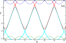
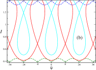
Figure 14: (Color version may be found in the online version of pre2008 as Fig. 9). Illustrations of the mechanisms of the formation of the 1st spike wings and of the corresponding theoretical lines in Fig. 15(a). Boxes (a), (b) and (c) illustrate the lines of Eqs. (104), (125) and (148) respectively: the corresponding perturbation parameters are ($\omega_{f}=0.39,h=0.0077$), ($\omega_{f}=0.41,h=0.00598$) and ($\omega_{f}=0.43,h=0.01009$) respectively. Resonance separatrices are drawn in red and cyan. The dashed lines show the functions $I_{\rm GSS}^{(l)}(\tilde{\psi})$ and $I_{\rm GSS}^{(u)}(\tilde{\psi})$. The black line in (c) is the trajectory of the resonant Hamiltonian system (87) which is tangent to both dashed lines.

If $\omega_{f}$ becomes slightly smaller than $\omega_{s}^{(j)}$, the resonances shift closer to the barriers while moving apart from each other. Hence, as $h$ increases, the overlap of the resonances with the chaotic layers associated with the barriers occurs earlier than with each other. Therefore, at $0<\omega_{s}^{(j)}-\omega_{f}\ll\omega_{m}$, the function $h_{gc}(\omega_{f})$ should correspond approximately to the reconnection of resonances of the order $n\equiv 2j-1$ (Fig. 14(a)). Fig. 15(a) demonstrates that even the asymptotic formula (106) for the separatrix reconnection line fits the left wing of the 1st spike quite well, and that the numerically calculated line (104) agrees with the simulations perfectly.

If $\omega_{f}$ becomes slightly larger than $\omega_{s}^{(j)}$ then, on the contrary, the resonances shift closer to each other and further from the barriers. Therefore, the mutual overlap of the resonances occurs at smaller $h$ than the overlap between any of them and the chaotic layer associated with the lower/upper barrier (cf. Figs. 10(c) and 10(d) as well as 11(c) and 11(d)). Hence, it is the latter overlap which determines the function $h_{gc}(\omega_{f})$ in the relevant range of $\omega_{f}$ (Fig. 14(b)). Fig. 15 shows that $h_{gc}(\omega_{f})$ is indeed well-approximated in the close vicinity to the right from $\omega_{s}^{(j)}$ by the numerical solution of Eq. (125) or (126), for an odd or even spike respectively and, for the 1st spike and the given $\Phi$, even by its asymptotic form,

$$h\equiv h(\omega_{f})=n\frac{-\Phi+\frac{\omega_{f}}{n\pi}\left[\Phi\left\{2\ln\left(\frac{4{\rm e}}{\Phi}\right)+\ln\left(\frac{\Phi+\Delta E^{(1)}}{\Phi-\Delta E^{(1)}}\right)\right\}-2\Delta E^{(1)}\right]}{2\sqrt{2}},$$

$$\Delta E^{(1)}\equiv\sqrt{\Phi^{2}-64\exp(-\frac{n\pi}{\omega_{f}})},n\equiv 2j-1,\quad|\omega_{f}-\omega_{s}^{(j)}|\ll\omega_{m}\,.$$ (146)

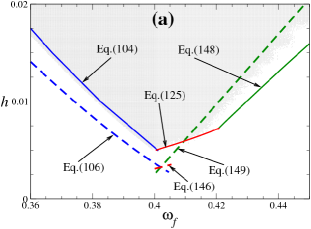
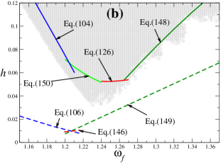
Figure 15: (Color version may be found in the online version of pre2008 as Fig. 10). The 1st (a) and 2nd (b) spike in $h_{gc}(\omega_{f})$: comparison between the results of the numerical simulations (the lower boundary of the shaded area) and the theoretical estimates. The estimates are indicated by the corresponding equation numbers and are drawn by different types of lines, in particular the dashed lines represent the explicit asymptote for the solid line of the same color.

The mechanism described above determines $h_{gc}(\omega_{f})$ only in the close vicinity of $\omega_{s}^{(j)}$. If $\omega_{f}/n$ becomes too close to $\omega_{m}$ or exceeds it, then the resonances are not of immediate relevance: they may even disappear or, if they still exist, their closed loops shrink, so that they can no longer provide for connection of the chaotic layers in the relevant range of $h$. At the same time, the closeness of the frequency to $\omega_{m}$ may still give rise to a large variation of action along the trajectory of the Hamiltonian system (87). For the odd/even spikes, the boundaries of the chaotic layers in the asymptotic limit $\Phi\rightarrow 0$ are formed in this case by the trajectory of (87) which is tangent to the lower/upper GSS curves (for the lower/upper layer) or by the lower/upper part of the separatrix of (87) generated by the saddle “$\tilde{s}$”/“$s$” (for the upper/lower layer). The overlap of the layers occurs when these trajectories coincide with each other, which may be formulated as the equality of $\tilde{H}$ in the corresponding tangency and saddle:

$$\tilde{H}(I_{t}^{(l)},\tilde{\psi}_{t}^{(l)})=\tilde{H}(I_{\tilde{s}},\tilde{\psi}_{\tilde{s}})\quad{\rm for}\quad j=1,3,5,\ldots,$$

$$\tilde{H}(I_{s},\tilde{\psi}_{s})=\tilde{H}(I_{t}^{(u)},\tilde{\psi}_{t}^{(u)})\quad{\rm for}\quad j=2,4,6,\ldots,$$

$$I_{\tilde{s}}\equiv I(E_{b}^{(2)}-\delta_{\tilde{s}}),\quad\quad I_{s}\equiv I(E_{b}^{(1)}+\delta_{s}).$$ (147)

Note however that, for moderately small $\Phi$, the tangencies may be relevant both to the lower layer and to the upper one (see the Appendix). Indeed, such a case occurs for our example with $\Phi=0.2$: see Fig. 14(c). Therefore, the overlap of the layers corresponds to the equality of $\tilde{H}$ in the tangencies:

$$\tilde{H}(I_{t}^{(l)},\tilde{\psi}_{t}^{(l)})=\tilde{H}(I_{t}^{(u)},\tilde{\psi}_{t}^{(u)})\,.$$ (148)

To the lowest order, Eq. (147) and Eq. (148) read as:

$$h\equiv h(\omega_{f})=\frac{\sqrt{2}\Phi\ln\left(\frac{4{\rm e}}{\Phi}\right)}{\pi}\left(\omega_{f}-\frac{n\pi}{2\ln\left(\frac{4{\rm e}}{\Phi}\right)}\right).$$ (149)

Both the line (148) and the asymptotic line (149) well agree with the part of the right wing of the 1st spike situated to the right from the fold at $\omega_{f}\approx 0.42$ (Fig. 15(a)). The fold corresponds to the change of the mechanisms of the chaotic layers overlap.

b]

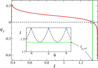
Figure 16: (Color version may be found in the online version of pre2008 as Fig. 11). Amplitude of the 3rd Fourier harmonic as a function of action (solid red line). The dashed black line shows the zero level. Its intersection with the solid red line is marked by the circle. The green line indicates the value of action where $q_{3}=0$. The inset illustrates the line (150) in Fig. 15(b): the GSS curve touches the horizontal line $I=I_{q_{3}=0}$.

If $\Phi$ is moderately small while $n>1$, the description of the far wings by the numerical lines (104) and (148) may be still quite good but the asymptotic lines (106) and (149) cannot pretend to describe the wings quantitatively any more (Fig. 15(b)). As for the minimum of the spike and the wings in its close vicinity, one more mechanism may become relevant for their formation (Figs. 15(b) and 16). It may be explained as follows. If $n>1$, then $q_{n}(E)$ becomes zero in the close vicinity ($\sim\Phi^{2}$) of the relevant barrier (the upper or lower barrier, in the case of even or odd spikes respectively: cf. Fig. 16). It follows from the equations of motion (98) that no trajectory can cross the line $I=I_{q_{n}=0}$. In the asymptotic limit $\Phi\rightarrow 0$, provided $h$ is from the range relevant for the spike minimum, almost the whole GSS curve is further from the barrier than the line $I=I_{q_{n}=0}$, and the latter becomes irrelevant. But, for a moderately small $\Phi$, the line may separate the whole GSS curve from the rest of the phase space. Then the resonance separatrix cannot connect to the GSS curve even if there is a state on the latter curve with the same value of $\tilde{H}$ as on the resonance separatrix. For a given $\omega_{f}$, the connection then requires a higher value of $h$: for such a value, the GSS curve itself crosses the line $I=I_{q_{n}=0}$. In the relevant range of $h$, the resonance separatrix passes very close to this line, so that the connection is well approximated by the condition that the GSS curve touches this line (see the inset in Fig. 16):

$$\delta_{u}=E_{b}^{(2)}-E_{q_{2j-1}=0}\quad\quad{\rm for}\quad j=2,4,6,\ldots,$$

$$\delta_{l}=E_{q_{2j-1}=0}-E_{b}^{(1)}\quad\quad{\rm for}\quad j=3,5,7,\ldots.$$ (150)

This mechanism is relevant to the formation of the minimum of the 2nd spike at $\Phi=0.2$, and in the close vicinity of the spike on the left (Fig. 15(b)).

Finally, let us find explicitly the universal asymptotic shape of the spike in the vicinity of its minimum. First, we note that the lowest-order expression (146) for the spike between the minimum and the fold can be written as the half-sum of the expressions (106) and (149) (which represent the lowest-order approximations for the spike to the left of the minimum, and to the right of the fold respectively). Thus, all three lines (106), (146) and (149) intersect at a single point. This means that, in the asymptotic limit $\Phi\rightarrow 0$, the fold merges with the minimum: $\omega_{f}$ and $h$ in the fold asymptotically approach $\omega_{s}$ and $h_{s}$ respectively. Thus, though the fold is a generic feature of the spikes, it is not of major significance: the spike is formed basically from two straight lines. The ratio between their slopes is universal. So, introducing a proper scaling, we reduce the spike shape to the universal function (Fig. 17):

$$\tilde{h}(\Delta\tilde{\omega}_{f})=\tilde{h}^{(lw)}(\Delta\tilde{\omega}_{f})\equiv 1-\sqrt{1-4{\rm e}^{c-2}}\Delta\tilde{\omega}_{f}\approx$$

$$\quad\quad\quad\quad\quad\quad\quad\quad\approx 1-0.593\Delta\tilde{\omega}_{f}\quad{\rm for}\quad\Delta\tilde{\omega}_{f}<0,$$

$$\tilde{h}(\Delta\tilde{\omega}_{f})=\tilde{h}^{(rw)}(\Delta\tilde{\omega}_{f})\equiv 1+\Delta\tilde{\omega}_{f}\quad{\rm for}\quad\Delta\tilde{\omega}_{f}>0,$$

(151)

$$\tilde{h}^{(fold)}(\Delta\tilde{\omega}_{f})=\frac{\tilde{h}^{(lw)}(\Delta\tilde{\omega}_{f})+\tilde{h}^{(rw)}(\Delta\tilde{\omega}_{f})}{2}\equiv$$

$$\equiv 1+\frac{1-\sqrt{1-4{\rm e}^{c-2}}}{2}\Delta\tilde{\omega}_{f}\approx 1+0.203\Delta\tilde{\omega}_{f},$$

$$\tilde{h}\equiv\frac{h}{h_{s0}},\quad\quad\Delta\tilde{\omega}_{f}\equiv\frac{\omega_{f}-\omega_{s1}}{\omega_{s1}-\omega_{s0}},\quad\quad\Phi\rightarrow 0,$$

where $\omega_{s0}$ and $h_{s0}$ are the lowest-order expressions (136) respectively for the frequency and amplitude in the spike minimum, $\omega_{s1}$ is the expression (139) for the frequency in the spike minimum, including the first-order correction, and $c$ is a constant (135).

b]

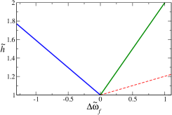
Figure 17: (Color version may be found in the online version of pre2008 as Fig. 12). The universal shape of the spike minimum (151) (solid lines). The dashed line indicates the universal slope of the spike in between the minimum and the fold, which have merged in the universal (asymptotic) function (151).

In addition to the left and right wings of the universal shape (the solid lines in Fig. 17), we include in (151) the function $\tilde{h}^{(fold)}(\Delta\tilde{\omega}_{f})$ (the dashed line in Fig. 17): its purpose is to show, on one hand, that the fold merges asymptotically with the minimum but, on the other hand, that the fold is generic and the slope of the spike between the minimum and the fold has a universal ratio to any of the slopes of the major wings.

Even for a moderately small $\Phi$, as in our example, the ratios between the three slopes related to the 1st spike in the simulations are reasonably well reproduced by those in Eq. (151): cf. Figs. 15(a) and 17. It follows from (151) that the asymptotic scaled shape is universal i.e. independent of $\Phi$ (but still assuming the asymptotic limit $\Phi\rightarrow 0$), $n$ or any other parameter.

The description of the wings of the spikes near their minima, in particular the derivation of the spike universal shape, constitutes the third main result of this section.

4.3 Generalizations and Applications

The facilitation of the onset of global chaos between adjacent separatrices has a number of possible generalizations and applications. We discuss an application in Sec. 5, but first list some of generalizations below.

1. The spikes in $h_{gc}(\omega_{f})$ may occur for an arbitrary Hamiltonian system with two or more separatrices. The asymptotic theory can be generalized accordingly.

2. The absence of pronounced spikes at even harmonics $2j\omega_{m}$ is explained by the symmetry of the potential (84): the even Fourier harmonics of the coordinate, $q_{2j}$, are equal to zero. For time-periodic perturbation of the dipole type, as in Eq. (85), there are no resonances of even order on account of this symmetry Chirikov:79 ; lichtenberg_lieberman ; Zaslavsky:1991 ; zaslavsky:1998 ; zaslavsky:2005 ; PR . If either the potential is non-symmetric, or the additive perturbation of the Hamiltonian is not an odd function of the coordinate, then even-order resonances do exist, resulting in the presence of the spikes in $h_{gc}(\omega_{f})$ at $\omega_{f}\approx 2j\omega_{m}$.

3. There may also be an additional facilitation of the onset of global chaos that could reasonably be described as a “secondary” facilitation. Let the frequency $\omega_{f}$ be close to the frequency $\omega_{s}$ of the spike minimum, while the amplitude $h$ be $\sim h_{s}$ but still lower than $h_{gc}(\omega_{f})$. Then there are two resonance separatrices in the $I-\tilde{\psi}$ plane that are not connected by chaotic transport (cf. Fig. 11(b)). This system possesses the zero-dispersion property. The trajectories of the resonant Hamiltonian (87) which start in between the separatrices oscillate in $I$ (as well as in ${\rm d}\tilde{\psi}/{\rm d}t$). The frequency $\tilde{\omega}$ of such oscillations along a given trajectory depends on the corresponding value of $\tilde{H}$ analogously to the way in which $\omega$ depends on $E$ for the original Hamiltonian $H_{0}$: $\tilde{\omega}(\tilde{H})$ is equal to zero for the values of $\tilde{H}$ corresponding to the separatrices (being equal in turn to $\tilde{H}_{sl}$ and $\tilde{H}_{su}$: see Eq. (103)) while possessing a nearly rectangular shape in between, provided the quantity $|\tilde{H}_{sl}-\tilde{H}_{su}|$ is much smaller than the variation of $\tilde{H}$ within each of the resonances,

   $$|\tilde{H}_{sl}-\tilde{H}_{su}|\ll\tilde{H}_{var}\sim|\tilde{H}_{sl}-\tilde{H}_{el}|\sim|\tilde{H}_{su}-\tilde{H}_{eu}|,$$ (152)

   where $\tilde{H}_{el}$ and $\tilde{H}_{eu}$ are the values of $\tilde{H}$ at the elliptic point of the lower and upper resonance respectively. The maximum of $\tilde{\omega}(\tilde{H})$ in between $\tilde{H}_{sl}$ and $\tilde{H}_{su}$ is described by the asymptotic formula:

   $$\tilde{\omega}_{m}\approx\frac{\pi}{\ln\left(\tilde{H}_{var}/|\tilde{H}_{sl}-\tilde{H}_{su}|\right)}.$$ (153)

   If we additionally perturb the system in such a way that an additional time-periodic term of frequency $\tilde{\omega}_{f}\approx\tilde{\omega}_{m}$ arises in the resonance Hamiltonian, then the chaotic layers associated with the resonance separatrices may be connected by chaotic transport even for a rather small amplitude of the additional perturbation, due to a scenario similar to the one described in this paper.

   There may be various types of such additional perturbation webs . For example, one may add to $H$ (85) one more dipole time-periodic perturbation of mixed frequency (i.e. $\approx\omega_{m}+\tilde{\omega}_{m}$). Alternatively, one may directly perturb the angle of the original perturbation by a low-frequency perturbation, i.e. the time-periodic term in $H$ (85) is replaced by the term

   $$-hq\cos(\omega_{f}t+A\cos(\tilde{\omega}_{f}t)),\quad\quad\omega_{f}\approx\omega_{m},\quad\quad\tilde{\omega}_{f}\approx\tilde{\omega}_{m}.$$ (154)

   Recently discussed physical problems where a similar situation is relevant are: chaotic mixing and transport in a meandering jet flow prants and reflection of light rays in a corrugated waveguide leonel .

4. If the time-periodic perturbation is multiplicative rather than additive, the resonances become parametric (cf. Landau:76 ). Parametric resonance is more complicated and much less studied than nonlinear resonance. Nevertheless, the main mechanism for the onset of global chaos remains the same, namely the combination of the reconnection between resonances of the same order and of their overlap in energy with the chaotic layers associated with the barriers. At the same time, the frequencies of the main spikes in $h_{gc}(\omega_{f})$ may change (though still being related to $\omega_{m}$). We consider below an example when the periodically driven parameter is $\Phi$ in (84). The Hamiltonian is

   $$H=p^{2}/2+(\Phi-\sin(q))^{2}/2,$$

   $$\Phi=\Phi_{0}+h\cos(\omega_{f}t),\quad\quad\Phi_{0}={\rm const}<1.$$ (155)

   The term $(\Phi-\sin(q))^{2}/2$ in $H$ (155) may be rewritten as $(\Phi_{0}-\sin(q))^{2}/2+(\Phi_{0}-\sin(q))h\cos(\omega_{f}t)+h^{2}\cos^{2}(\omega_{f}t)/2$. The last term in the latter expression does not affect the equations of motion. Thus, we end up with an additive perturbation $(\Phi_{0}-\sin(q))h\cos(\omega_{f}t)$. In the asymptotic limit $\Phi_{0}\rightarrow 0$, the $n$th-order Fourier component of the function $(\Phi_{0}-\sin(q))$ can be shown to differ from zero only for the orders $n=2,6,10,...$ Therefore one may expect the main spikes in $h_{gc}(\omega_{f})$ to be at frequencies twice larger than those for the dipole perturbation (85):

   $$\omega_{sp}^{(j)}\approx 2\omega_{s}^{(j)}\approx 2(2j-1)\omega_{m},\quad\quad j=1,2,3,...$$ (156)

   This agrees well with the results of simulations (Fig. 18).

   t]

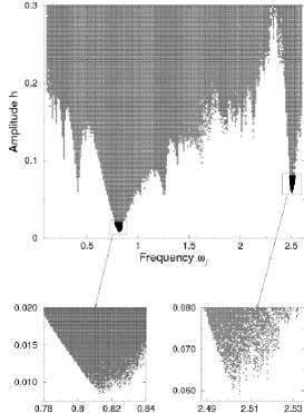
   Figure 18: Diagram analogous to that in Fig. 9, but for the system (155) (with $\Phi_{0}=0.2$).

   Moreover, the asymptotic theory for the dipole perturbation may immediately be generalized to the present case: it is necessary only to replace the Fourier component of the coordinate $q$ by the Fourier component of the function $(\Phi_{0}-\sin(q))$:

   $$(\Phi_{0}-\sin(q))_{n}=\left\{{}_{0\quad\quad{\rm at}\quad n\neq 2(2j-1),}^{\frac{4}{\pi n}\quad{\rm at}\quad n=2(2j-1),}\right.\quad\quad j=1,2,3,...,\quad\quad\Phi_{0}\rightarrow 0$$ (157)

   (cf. Eq. (96) for $q_{n}$). We obtain:

   $$\omega_{sp0}\equiv\omega_{sp0}^{\left(\frac{n+2}{4}\right)}=n\frac{\pi}{2\ln\left(\frac{4{\rm e}}{\Phi_{0}}\right)},\quad\quad h_{sp0}\equiv h_{sp0}^{\left(\frac{n+2}{4}\right)}=n\frac{c\pi}{8}\frac{\Phi_{0}}{\ln\left(\frac{4{\rm e}}{\Phi_{0}}\right)},$$ (158)

   $$n=2,6,10,...,\qquad\Phi_{0}\rightarrow 0,$$

   where $c$ is given in Eqs. (134) and (135).

   For $\Phi_{0}=0.2$, Eq. (158) gives, for the 1st spike, values differing from the simulation data by about $3\%$ in frequency and by about $10\%$ in amplitude. Thus, the lowest-order formulæ accurately describe the 1st spike even for a moderately small $\Phi$.

5. One more generalization relates to multi-dimensional Hamiltonian systems with two or more saddles with different energies: the perturbation may not necessarily be time-periodic, in this case. The detailed analysis has not yet been done.

The paper pre2008 presents a rather detailed discussion of possible applications to the telectron gas in a magnetic superlattice, a spinning pendulum, cold atoms in an optical lattice as well as to problems of noise-induced escape and the stochastic web formation. We review briefly in the next section the further development of the latter application.

5 Enlargement of a low-dimensional stochastic web

The stochastic web concept dates back to the 1960s when Arnold showed arnold that, in non-degenerate Hamiltonian systems of dimension exceeding 2, resonance lines necessarily intersect, forming an infinite-sized web in the Poincaré section. It provides in turn for a slow chaotic (sometimes called “stochastic”) diffusion for infinite distances in relevant dynamical variables.

It was discovered towards the end of 1980s zaslavsky:1986 ; A.A. ; chernikov:1987_ ; chernikov:1988 that, in degenerate or nearly-degenerate systems, a stochastic web may arise even if the dimension is 3/2. One of the archetypal examples of such a low-dimensional stochastic web arises in the 1D harmonic oscillator perturbed by a weak traveling wave the frequency of which coincides with a multiple of the natural frequency of the oscillator zaslavsky:1998 ; chernikov:1987_ ; Zaslavsky:1991 . Perturbation plays a dual role: on the one hand, it gives rise to a slow dynamics characterized by an auxiliary Hamiltonian that possesses an infinite web-like separatrix; on the other hand, the perturbation destroys this self-generated separatrix, replacing it by a thin chaotic layer. Such a low-dimensional stochastic web may be relevant to a variety of physical systems and plays an important role in corresponding transport phenomena: see zaslavsky:1998 ; chernikov:1987_ ; Zaslavsky:1991 for reviews on relevant classical systems. In addition, there are quantum systems in which the dynamics of transport reduces to that in the classical model described above. The latter concerns e.g. nanometre-scale semiconductor superlattices with an applied voltage and magnetic field fromhold ; fromhold_nature .

One might assume that, like the Arnold web, the low-dimensional stochastic web described above should be infinite, so that it can provide for transport between the centre of the web and states situated arbitrarily far away in coordinate and momentum. However the numerical integration of the equations of motion shows that this is not so: even for a rather non-weak perturbation, the real web is limited to the region within a few inner loops of the infinite web-like resonant separatrix (Fig. 19(a)) while chaotic layers associated with outer loops are distinctly separated from each other and from the web-like chaotic layer formed by the few inner loops. The reason is apparently as follows. The single infinite web-like separatrix is possessed by the resonant Hamiltonian only in the first-order approximation of the averaging method bogmit whereas, with the account taken of the next-order approximations, the separatrix apparently splits into many separate complex loops successively embedded into each other. Non-resonant terms of the perturbation dress the separatrices by exponentially narrow chaotic layers. If the perturbation is not small, the chaotic layers manage to connect neighbouring separatrix loops situated close to the centre. However, the width of the chaotic layer decreases exponentially sharply as the distance from the centre grows zaslavsky:1998 ; chernikov:1987_ ; Zaslavsky:1991 . As a result, the merger between chaotic layers associated with neighbouring loops takes place only within the few loops closest to the centre, provided that the perturbation is not exponentially strong.

If the resonance between the perturbation and the oscillator is inexact, or if the oscillator is nonlinear, the splitting between the neighbouring loops is typically much larger: it appears even in the first-order approximation of the averaging method zaslavsky:1998 ; chernikov:1988 ; Zaslavsky:1991 . So the number of loops connected to the centre by chaotic transport is even smaller zaslavsky:1998 ; chernikov:1988 ; Zaslavsky:1991 than in the case of the exact resonance.

A natural question arises: how can the perturbation be modified in order for the transport to be unlimited or, at least, significantly extended? One of the answers was obtained in the very beginning of studies of the low-dimensional webs zaslavsky:1986 ; A.A. : if the perturbation consists of repeated in time short kicks that are also periodic space, and if the frequency of the kicks is equal to a multiple of the natural frequency, then a so-called uniform web covering the whole of phase space is formed. However such a perturbation is absent in many cases and, even where present, the chaotic transport is still exponentially slow if the perturbation is weak zaslavsky:1998 ; Zaslavsky:1991 .

It is reasonable then to pose the following question: is it possible to obtain a web of form similar to the original one chernikov:1987_ but substantially extended in phase space? A positive answer was suggested in pre2008 and explicitly realized recently icnf_enlargement using the following simple idea. The chaotic layer in the webs is exponentially narrow since the frequency of the non-resonant perturbation of the resonant Hamiltonian is necessarily much higher than the frequency of small eigenoscillation in the cell of the web-like separatrix zaslavsky:1998 ; zaslavsky:1986 ; A.A. ; chernikov:1987_ ; chernikov:1988 ; Zaslavsky:1991 . So we need to modify the perturbation in such a way that the resonant Hamiltonian does not change while its perturbation contains, in addition to the conventional terms, a low-frequency one. One may do this modulating the wave angle with a low frequency or adding one more wave with the frequency slightly shifted from the original one. The latter option, together with a generalization for the uniform web leading to a huge enhancement of the chaotic transport through it, have not yet been considered in detail while the work icnf_enlargement and the present section concentrate on the former option since it may have immediate applications to nanometre-scale semiconductor superlattices in electric and magnetic fields fromhold ; fromhold_nature .

5.1 Slow modulation of the wave angle

Fig. 19 demonstrates the validity of our idea. We integrate the equation

$$\ddot{q}+q=0.1\sin[15q-4t-h\sin(0.02t)],$$ (159)

first for $h=0$ (i.e. for the conventional case with parameters as in zaslavsky:1998 ; chernikov:1987_ ; Zaslavsky:1991 ), and secondly for $h=0.1$. Although the modulation in the latter case is weak (its amplitude is about 63 times smaller than the $2\pi$ period of the wave angle which is a characteristic scale in this problem), the resultant increase in the size of the web in coordinate and momentum is large: by a factor of $\sim$6.

An analytic theory can be developed to account for these results. It can be generalized for the off-resonant case zaslavsky:1998 ; chernikov:1988 ; Zaslavsky:1991 too, using the general method developed in pre2008 ; proceedings ; icnf_approach ; pre_submitted and described above in the previous sections.

It is anticipated that the method can also be generalized for uniform webs zaslavsky:1998 ; zaslavsky:1986 ; Zaslavsky:1991 too, leading to an exponentially strong enhancement of chaotic transport through them.

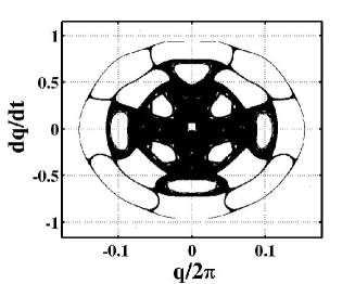
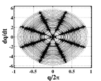
Figure 19: The Poincaré section for a trajectory of the system (159) with initial state $q=0.1,\;\dot{q}=0$ (at instants $t_{n}=nT$ where $T\equiv 2\pi/0.02$ is the period of the modulation and $n=1,2,3,...600000$) for $h=0$ (left panel) and $h=0.1$ (right panel). A sympletic integration scheme of the fourth order is used, with an integration step $t_{int}=\frac{2\pi}{40000}\approx 1.57\times 10^{-4}$, so that the inaccuracy at each step is of the order of $t_{int}^{5}\approx\times 10^{-19}$. The left panel corresponds to the example of the conventional case considered in zaslavsky:1998 ; chernikov:1987_ ; Zaslavsky:1991 . The right panel demonstrates that the modulation, although weak, greatly enlarges the web sizes.

5.2 Application to semiconductor superlattices

The works fromhold ; fromhold_nature consider quantum electron transport in 1D semiconductor superlattices (SLs) on the nanometre scale, subject to a constant electric field along the SL axis and to a constant magnetic field. The spatial periodicity with a period of the nanometre scale gives rise to the onset of minibands for electrons. In the tight-binding approximation, the electron motion in the lowest mini-band is described by the following dispersion relation for the electron energy $E$ versus momentum $\vec{p}$:

$$E(\vec{p})=\frac{\Delta[1-\cos(p_{x}d/\hbar)]}{2}+\frac{p_{y}^{2}+p_{z}^{2}}{2m^{*}},$$ (160)

where $x$ is the direction along the SL axis, $\Delta$ is the miniband width, $d$ is the SL period, $m^{*}$ is the electron effective mass for the motion in the transverse (i.e. $y-z$) direction.

Thus, the quasi-classical motion of electron in an electric field $\vec{F}$ and a magnetic field $\vec{B}$ is described by the following equation:

$$\frac{{\rm d}\vec{p}}{{\rm d}t}=-e\{\vec{F}+[\nabla_{\vec{p}}E(\vec{p})\times\vec{B}]\}.$$ (161)

where $e$ is the electron charge

It was shown in fromhold that, with a constant electric field along the SL axis $\vec{F}=(-F_{0},0,0)$ and a constant magnetic field with a given angle $\theta$ to the axis $\vec{B}=(B\cos(\theta),0,B\sin(\theta))$, the dynamics of the $z$-component of momentum $p_{z}$ reduces to the equation of motion of an auxiliary harmonic oscillator in a plane wave. At certain values of the parameters, the ratio of the wave and oscillator frequencies takes integer values (like in Eq. (159) with $h=0$) which gives rise to the onset of the stochastic web, leading in turn to a delocalization of the electron in the $x$-direction and, as a result, to an increase of the dc-conductivity along the SL axis. The experiment fromhold_nature appears to provide evidence in favor of this exciting hypothethis.

At the same time, the finite size of the web and, yet more so, the exponentially fast decrease in the transport rate as the distance from the centre of the web increases, seems to put strong limitations on the use of the effect. We suggest a simple and efficient way to overcome these limitations. Indeed, one can show that, if we add to the original (constant) electric field $F_{0}$ a small time-periodic (ac) component $F_{\rm ac}\sin(\Omega_{\rm ac}t)$, then the wave angle in the equation of motion of $p_{z}$ is modulated by the term (cf. Eq. (159)):

$$h\sin(\Omega t)\equiv\frac{F_{\rm ac}}{F_{0}}\frac{\Omega_{0}}{\Omega_{\rm ac}}\sin\left(\frac{\Omega_{\rm ac}}{\Omega_{0}}t\right),\quad\quad\Omega_{0}\equiv\frac{eF_{0}d}{\hbar}.$$ (162)

This allows us to increase drastically the size of the web and the rate of chaotic transport through it. For example, for the case shown in Fig. 19, where we have an increase of the web size by a factor of 6$\times$, it is sufficient to add an ac component of the electric field with the frequency $0.02\cdot\Omega_{0}$ and an amplitude $F_{\rm ac}=0.1\cdot 0.02\cdot F_{0}$ i.e. an amplitude smaller than that of the original constant field $F_{0}$ by a factor of 500$\times$.

5.3 Discussion

We have presented above just initial results on the subject icnf_enlargement . There are still many unsolved interesting problems –

1. It can be shown that, in the off-resonance case, there may be a facilitation of the onset of global chaos similar to that described in Sec. 4 above, i.e. the critical value of the modulation amplitude $h$ required for the onset of global chaos between neighbouring separatrix loops possesses deep spikes (minima) as a function of the modulation frequency $\Omega_{ac}$. The detailed theory of this facilitation has yet to be developed.

2. Our conjecture that, in the resonant case, taking account of the next-order approximations of the averaging method could explain the split between different separatrix loops, should be proved rigorously. If the corresponding theory is developed, it will provide the possibility of calculating both the optimal modulation frequency, i.e. that at which the web sizes are maximal, for a given amplitude of modulation, and the maximum sizes themselves.

3. It would be interesting to study the case with an additive perturbation (rather than an angular modulation) in detail, both numerically and theoretically.

6 Conclusions

We have reviewed the recently developed method for the theoretical treatment of separatrix chaos in regimes when it involves resonance dynamics. It has been applied both to single-separatrix chaotic layers and to the onset of global chaos between two close separatrices. The method is based on a matching between the discrete chaotic dynamics of the separatrix map and the continuous regular dynamics of the resonance Hamiltonian. For single-separatrix chaos, the method has allowed:

1. Development of the first asymptotic (i.e. for $h\rightarrow 0$) description of the high peaks in the width of the separatrix chaotic layer as a function of the perturbation frequency, thus describing its dominant feature and, in particular, its maxima.

2. Classification of all systems into two types, based on the asymptotic dependence of the maximum width on the perturbation amplitude $h$: the maximum width is proportional to $h\ln(1/h)$ or $h$ for systems of type I or type II respectively.

For systems with two or more separatrices, the method has allowed us to develop an accurate asymptotic theory of the facilitation of the onset of global chaos between neighbouring separatrices which occurs at frequencies close to multiples of a local maximum in the eigenoscillation frequency as a function of the energy: the local maximum necessarily exists in the range between the separatrices.

Finally, for an oscillator perturbed by a plane wave of frequency equal to or close to the frequency of a small eigenoscillation, the method has allowed us to suggest how to enlarge substantially the size of the stochastic web using a rather weak perturbation, and it promises to provide an accurate theoretical description of the enlargement.

7 Appendix

This appendix follows the appendix of the paper pre2008 . The chaotic layers of the system (85) associated with the separatrices of the unperturbed system (84) are described here by means of the separatrix map. To derive the map, we follow the method described in Zaslavsky:1991 , but the analysis of the map significantly differs from formerly existing ones lichtenberg_lieberman ; Zaslavsky:1991 ; zaslavsky:1998 ; zaslavsky:2005 ; treschev (cf. also the recently published paper shevchenko where the analysis of the map has some similarity to ours but still differs significantly). Using our approach, we are able to calculate the chaotic layer boundaries in the phase space (rather than only in energy), throughout the resonance frequency ranges, and we can quantitatively describe the transport within the layer in a manner different from existing ones (cf. treschev ; vered1 and references therein).

7.1 Lower chaotic layer

.

We now present a detailed consideration of the lower chaotic layer. The upper layer may be considered in a very similar way.

Separatrix map

A typical form of trajectory $\dot{q}(t)$ close to the inner separatrix (that corresponding to the lower potential barrier) is shown in Fig. 20. One can resolve pulses in $\dot{q}(t)$. Each of them consists of two approximately antisymmetric spikes. The pulses are separated by intervals during which $|\dot{q}|$ is relatively small. In general, successive intervals differ between each other. Let us introduce the pair of variables $\,E\,$ and $\,\varphi$:

t]

Figure 20: Schematic example of the time dependence of the velocity of the perturbed system (thick solid line) in the case when the energy of motion varies in the close vicinity of the top of the lower potential barrier. The dashed line marks the zero level of the velocity. Pulses of the velocity are schematically singled out by the parallelograms (drawn by a thin solid line). The two sequences of time instants $(...,t_{i-1},t_{i},t_{i+1},...)$ and $(...,t_{i-1}^{\prime},t_{i}^{\prime},t_{i+1}^{\prime},...)$ correspond to beginnings and centers of the pulses, respectively.

$$E\equiv H_{0},\quad\varphi\equiv\omega_{f}t+\varphi_{a}\,,$$ (163)

where the constant $\varphi_{a}$ may be chosen arbitrarily.

The energy $E$ changes only during the pulses of $\dot{q}(t)$ and remains nearly unchanged during the intervals between the pulses, when $|\dot{q}(t)|$ is small Zaslavsky:1991 . We assign numbers $\,i\,$ to the pulses and introduce the sequences of $(E_{i},\varphi_{i})$ corresponding to the initial instants $t_{i}$ of the pulses. In such a way, we obtain the following map (cf. Zaslavsky:1991 ):

$$E_{i+1}=E_{i}+\Delta E_{i},\quad\quad\varphi_{i+1}=\varphi_{i}+\frac{\omega_{f}\pi(3-{\rm sign}(E_{i+1}-E_{b}^{(1)}))}{2\omega(E_{i+1})},$$

$$\Delta E_{i}\equiv h\int_{\hbox{\small{{\it i\,}th pulse}}}\!\!\!\!\!{\rm d}t\;\dot{q}(t)\cos(\omega_{f}t),$$ (164)

where $\,\int_{\hbox{\small{{\it i\,}th pulse}}}\,$ means integration over the $i$th pulse. Before deriving a more explicit expression for $\Delta E_{i}$, we make two remarks.

1. Let us denote with $t_{i}^{\prime}$ the instant within the $i$th pulse when $\dot{q}$ is equal to zero (Fig. 20). The function $\dot{q}(t-t_{i}^{\prime})$ is an odd function within the $i$th pulse and it is convenient to transform the cosine in the integrand in $\Delta E_{i}$ (164) as

   $$\cos(\omega_{f}t)\equiv\cos(\omega_{f}(t-t_{i}^{\prime})+\omega_{f}t_{i}^{\prime})\equiv\cos(\omega_{f}(t-t_{i}^{\prime}))\cos(\omega_{f}t_{i}^{\prime})-\sin(\omega_{f}(t-t_{i}^{\prime}))\sin(\omega_{f}t_{i}^{\prime}),$$

   and to put $\varphi_{a}=\omega_{f}(t_{i}^{\prime}-t_{i})$, so that $\varphi_{i}\equiv\omega_{f}t_{i}^{\prime}$.

2. Each pulse of $\dot{q}$ contains one positive and one negative spike. The first spike can be either positive or negative. If $E$ changes during the given $n$th pulse so that its value at the end of the pulse is smaller than $E_{b}^{(1)}$, then the first spikes of the $i$th and $(i+1)$st pulses have the same signs. On the contrary, if $E$ at the end of the $i$th pulse is larger than $E_{b}^{(1)}$, then the first spikes of the $i$th and $(i+1)$st pulses have opposite signs. Note that Fig. 20 corresponds to the case when the energy remains above $E_{b}^{(1)}$ during the whole interval shown in the figure. This obviously affects the sign of $\Delta E_{i}$, and it may be explicitly accounted for in the map if we introduce a new discrete variable $\sigma_{i}=\pm 1$ which characterizes the sign of $\dot{q}$ at the beginning of a given $i$th pulse,

   $$\sigma_{i}\equiv{\rm sign}(\dot{q}(t_{i}))\ ,$$ (165)

   and changes from pulse to pulse as

   $$\sigma_{i+1}=\sigma_{i}\,{\rm sign}(E_{b}^{(1)}-E_{i+1})\ .$$ (166)

With account taken of the above remarks, we can rewrite the map (164) as follows:

$$E_{i+1}=E_{i}+\sigma_{i}h\epsilon^{(low)}\sin(\varphi_{i}),$$ (167)

$$\varphi_{i+1}=\varphi_{i}+\frac{\omega_{f}\pi(3-{\rm sign}(E_{i+1}-E_{b}^{(1)}))}{2\omega(E_{i+1})},$$

$$\sigma_{i+1}=\sigma_{i}\,{\rm sign}(E_{b}^{(1)}-E_{i+1}),$$

$$\quad\quad\;\epsilon^{(low)}\equiv\epsilon^{(low)}(\omega_{f})=-\sigma_{i}\int_{i{\rm th}\;{\rm pulse}}{\rm d}t\;\dot{q}(t-t_{i}^{\prime})\sin(\omega_{f}(t-t_{i}^{\prime}))$$

$$\quad\quad\quad\quad\quad\quad\approx-2\sigma_{i}\int_{t_{i}^{\prime}}^{t_{i+1}}{\rm d}t\;\dot{q}(t-t_{i}^{\prime})\sin(\omega_{f}(t-t_{i}^{\prime})).$$

A map similar to (167) was introduced in ZF:1968 , and it is often called the Zaslavsky separatrix map. It was re-derived mathematically rigorously in vered ; see also the recent mathematical review treschev . The latter review also describes generalizations of the Zaslavsky map as well as other types of separatrix map. The analysis presented below relates immediately to the Zaslavsky map but it is hoped that it will prove possible to generalize it for other types of separatrix maps too.

The variable $\epsilon^{(low)}$ introduced in (167) will be convenient for the further calculations since it does not depend on $i$ in the lowest-order approximation. A quantity like $\delta_{l}\equiv h|\epsilon^{(low)}|$ is sometimes called the separatrix split zaslavsky:1998 since it is conventionally assumed that the maximal deviation of energy on the chaotic trajectory from the separatrix energy is of the order of $\delta_{l}$ lichtenberg_lieberman ; Zaslavsky:1991 ; zaslavsky:1998 ; zaslavsky:2005 . As in the main text, we shall use this term, but we emphasize that the maximal deviation may be much larger.

In the adiabatic limit $\omega_{f}\rightarrow 0$, the excess of the upper boundary $E_{cl}^{(1)}$ of the lower layer over the lower barrier $E_{b}^{(1)}$ does not depend on angle and is equal to $2\pi h$ (cf. E&E:1991 ). But $\omega_{f}$ relevant for the spike of $h_{gc}(\omega_{f})$ cannot be considered as an adiabatic frequency, despite its smallness, because it is close to $\omega_{m}$ or to its multiple while all energies at the boundary lie in the range where the eigenfrequency is also close to $\omega_{m}$:

$$\omega_{f}\approx(2j-1)\omega_{m}\approx(2j-1)\omega(E_{cl}^{(1)}),\quad\quad j=1,2,3,...$$ (168)

The validity of (168) (confirmed by the results) is crucial for the description of the layer boundary in the relevant case.

Separatrix split

Let us evaluate $\epsilon^{(low)}$ explicitly. Given that the energy is close to $E_{b}^{(1)}$, the velocity $\dot{q}(t-t_{i}^{\prime})$ in $\epsilon^{(low)}$ (167) may be replaced by the corresponding velocity along the separatrix associated with the lower barrier, $\dot{q}_{s}^{(low)}(t-t_{i}^{\prime})$, while the upper limit of the integral may be replaced by infinity. In the asymptotic limit $\Phi\rightarrow 0$, the interval between spikes within the pulse becomes infinitely long²³ so that only the short ($\sim\omega_{0}^{-1}$) intervals corresponding to the spikes contribute to the integral in $\epsilon^{(low)}$ (167). In the scale $\omega_{f}^{-1}$, they may be considered just as the two instants:

$$t_{sp}^{(1,2)}-t_{i}^{\prime}\approx\pm\frac{\pi}{4\omega_{m}},\quad\Phi\rightarrow 0.$$ (169)

In the definition of $\epsilon^{(low)}$ (167), we substitute the argument of the sine by the corresponding constants for the positive and negative spikes respectively:

$$\epsilon^{(low)}\approx 2\sin\left(\frac{\pi\omega_{f}}{4\omega_{m}}\right)\int_{\rm positive\,spike}{\rm d}t\;\dot{q}_{s}^{(low)}(t-t_{i}^{\prime})\approx 2\pi\sin\left(\frac{\pi\omega_{f}}{4\omega_{m}}\right),$$ (170)

$$\Phi\rightarrow 0.$$

In the derivation of the first equality in (170), we have also taken into account that the function $\dot{q}_{s}^{(low)}(x)$ is odd. In the derivation of the second equality in (170), we have taken into account that the right turning point of the relevant separatrix is the top of the lower barrier and the distance between this point and the left turning point of the separatrix approaches $\pi$ in the limit $\Phi\rightarrow 0$.

For the frequencies relevant to the minima of the spikes of $h_{gc}(\omega_{f})$, i.e. for $\omega_{f}=\omega_{s}^{(j)}\approx(2j-1)\omega_{m}$, we obtain:

$$\epsilon^{(low)}(\omega_{s}^{(j)})\approx 2\pi\sin\left((2j-1)\frac{\pi}{4}\right)=\sqrt{2}\pi(-1)^{\left[\frac{2j-1}{4}\right]},$$

$$j=1,2,3,...,\quad\Phi\rightarrow 0.$$ (171)

For moderately small $\Phi$, it is better to use the more accurate formula:

$$\epsilon^{(low)}(\omega_{f})=2\int_{0}^{\infty}{\rm d}t\;\dot{q}_{s}^{(low)}(t)\sin(\omega_{f}t),$$ (172)

where the instant $t=0$ corresponds to the turning point of the separatrix to the left of the lower barrier, i.e. $\dot{q}_{s}^{(low)}(t=0)=0$ while $\dot{q}_{s}^{(low)}>0$ for all $t>0$. The dependence $\left|\epsilon^{(low)}(\omega_{f})\right|$ by Eq. (172) is shown for $\Phi=0.2$ in Fig. 21(a). For small frequencies, the asymptotic formula (170) fits well the formula (172).

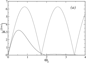
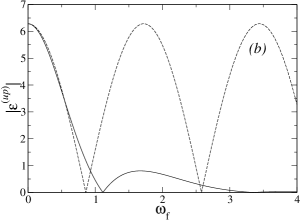
Figure 21: Theoretical estimates for the normalized separatrix split (for $\Phi=0.2$) as a function of the perturbation frequency, for the lower and upper layers in (a) and (b) respectively. The solid lines are calculated from Eqs. (172) and (204) for (a) and (b) respectively, while the dashed lines represent the asymptotic expressions (170) and (205) respectively.

Dynamics of the map

Consider the dynamics of the map (167) when $\omega_{f}$ is close to the spikes’ minima: $\omega_{f}\approx n\omega_{m}$ where $n\equiv 2j-1$ while $j=1,2,3,\ldots$. Let the energy at the step $i=-1$ be equal to $E_{b}^{(1)}$. The trajectory passing through the state with this energy is chaotic since $(\omega(E))^{-1}$ diverges as $E\rightarrow E_{b}^{(1)}$ and, therefore, the angle $\varphi_{-1}$ is not correlated with the angle on the previous step $\varphi_{-2}$. The quantity $\sigma_{-1}$ is not correlated with $\sigma_{-2}$ either. Thus, $\sin(\varphi_{-1})$ may take any value in the range $[-1,1]$ and $\sigma_{-1}$ may equally take the values 1 or -1. Therefore, the energy may change on the next step by an arbitrary value in the interval $[-h|\epsilon^{(low)}|,h|\epsilon^{(low)}|]$. Thus, $E_{0}-E_{b}^{(1)}$ may have a positive value $\sim h|\epsilon^{(low)}|$. Then, the approximate equality $n\omega(E_{0})\approx\omega_{m}$ holds, provided that the value of $h$ is from the relevant range. Allowing for this and recalling that we are interested only in those realizations of the map such that $E_{0}>E_{b}^{(1)}$, the relevant realization of the map $i=-1\;\rightarrow\;i=0$ may be written as:

$$E_{0} = E_{b}^{(1)}+\sigma_{-1}h\epsilon^{(low)}\sin(\varphi_{-1})=E_{b}^{(1)}+h|\epsilon^{(low)}\sin(\varphi_{-1})|,$$

$$\varphi_{0} \approx \varphi_{-1}+n\pi,$$

$$\sigma_{0} =-\sigma_{-1}.$$ (173)

One may expect that further evolution of the map will, for some time, approximately follow the trajectory of the system (87) with the initial energy $E_{0}$ (173) and an arbitrary $\varphi_{-1}$ and initial slow angle $\tilde{\psi}$ somehow related to $\varphi_{0}\approx\varphi_{-1}+n\pi$. Let us prove this explicitly.

Consider two subsequent iterations of the map (167): $2i\rightarrow 2i+1$ and $2i+1\rightarrow 2i+2$ with an arbitrary $i\geq 0$. While doing this, we shall assume the validity of (168) (it will be clarified below when this is true) from which it follows that: (i) $\omega(E_{k+1})\approx\omega(E_{k})$, (ii) $\varphi_{k+1}-\varphi_{k}\approx n\pi\equiv(2j-1)\pi$. It will follow from the results that the neglected corrections are small in comparison with the characteristic scales of the variation of $E$ and $\varphi$ (cf. the conventional treatment of the nonlinear resonance dynamics Chirikov:79 ; lichtenberg_lieberman ; Zaslavsky:1991 ; zaslavsky:1998 ; zaslavsky:2005 ; PR ). Furthermore it follows from (167) that, while the energy remains above the barrier energy, $\sigma_{k}$ oscillates, so that $\sigma_{2i}=\sigma_{0}$ and $\sigma_{2i+1}=-\sigma_{0}$. Then,

$$E_{2i+1} = E_{2i}+\sigma_{0}h\epsilon^{(low)}\sin(\varphi_{2i}),$$

$$\varphi_{2i+1} = \varphi_{2i}+\frac{\omega_{f}}{\omega(E_{2i+1})}\pi\approx\varphi_{2i}+n\pi+\pi\frac{\omega_{f}-n\omega(E_{2i})}{\omega(E_{2i})},$$ (174)

$$E_{2i+2} = E_{2i+1}-\sigma_{0}h\epsilon^{(low)}\sin(\varphi_{2i+1})=$$

$$= E_{2i+1}+\sigma_{0}h\epsilon^{(low)}\sin(\varphi_{2i+1}-n\pi)\approx E_{2i}+\sigma_{0}2h\epsilon^{(low)}\sin(\varphi_{2i}),$$

$$\varphi_{2i+2} = \varphi_{2i+1}+\frac{\omega_{f}}{\omega(E_{2i+2})}\pi\approx\varphi_{2i}+2\pi n+2\pi\frac{\omega_{f}-n\omega(E_{2i})}{\omega(E_{2i})}$$ (175)

(the second equality in the map for $E_{2i+2}$ takes into account that $n$ is odd so that $\sin(\varphi-n\pi)=-\sin(\varphi)$.)

The quantity $\varphi_{2i+2}-\varphi_{2i}-2\pi n$ is small, so the map $2i\rightarrow 2i+2$ (175) may be approximated by differential equations for $E_{2i}$ and $\tilde{\varphi}_{2i}\equiv\varphi_{2i}-2\pi ni$:

$$\frac{{\rm d}E_{2i}}{{\rm d}(2i)}=\sigma_{0}h\epsilon^{(low)}\sin(\tilde{\varphi}_{2i}),\quad\quad\frac{{\rm d}\tilde{\varphi}_{2i}}{{\rm d}(2i)}=\frac{\pi}{\omega(E_{2i})}(\omega_{f}-n\omega(E_{2i})),$$ (176)

$$\tilde{\varphi}_{2i}\equiv\varphi_{2i}-2\pi ni.$$

Let us (i) use for $\epsilon^{(low)}$ the asymptotic formula (171), (ii) take into account that the increase of $i$ by 1 corresponds to an increase of time by $\pi/\omega(E)$, and (iii) transform from the variables $(E,\tilde{\varphi})$ to the variables $(I,\tilde{\psi}\equiv n\pi(1-\sigma_{0})/2-\tilde{\varphi})$. Equations (176) reduce then to:

$$\frac{{\rm d}I}{{\rm d}t}=-h\sqrt{2}(-1)^{\left[\frac{n}{4}\right]}\sin(\tilde{\psi}),\quad\quad\frac{{\rm d}\tilde{\psi}}{{\rm d}t}=n\omega-\omega_{f},$$ (177)

$$\tilde{\psi}\equiv n\pi\frac{1-\sigma_{0}}{2}-\tilde{\varphi},\quad\quad n\equiv 2j-1.$$

Equations (177) are identical to the equations of motion of the system (87) in their lowest-order approximation, i.e. to equations (98) where $q_{n}$ is replaced by its asymptotic value (96) and the last term in the right-hand part of the second equation is neglected, being of higher order in comparison with the term $n\omega-\omega_{f}$.

Apart from the formal identity of Eqs. (177) and (98), $\tilde{\psi}$ in (177) and $\tilde{\psi}$ in (98) are identical to. Necessarily $t_{i}^{\prime}$ corresponds to a turning point (see Fig. 20) while the corresponding $\psi$ is equal to $2\pi i$ or $\pi+2\pi i$ for the right and left turning points respectively (see (87)) i.e. $\psi=2\pi i+\pi(1-\sigma_{i})/2$, so that $\tilde{\psi}_{(98)}\equiv n\psi-\omega_{f}t=n\pi(1-\sigma)/2-\tilde{\varphi}\equiv\tilde{\psi}_{(177)}$.

The relevant initial conditions for (177) follow from (173) and from the relationship between $\tilde{\psi}$ and $\varphi$:

$$I(0)=I(E=E_{b}^{(1)}+h\sqrt{2}\pi|\sin(\tilde{\psi}(0))|),$$ (178)

while $\tilde{\psi}(0)\equiv n\pi(1-\sigma_{0})/2-\varphi_{0}$ may be an arbitrary angle from the ranges where

$$(-1)^{[n/4]}\sin(\tilde{\psi}(0))<0.$$ (179)

For moderately small $\Phi$, it is better to use the more accurate dynamic equations (98) instead of (177) and the more accurate initial value of action instead of (178):

$$I(0)=I(E=E_{b}^{(1)}+\delta_{l}|\sin(\tilde{\psi}(0))|),\quad\quad\delta_{l}\equiv h|\epsilon^{(low)}|,$$ (180)

with $\epsilon^{(low)}$ calculated by (172).

We name the quantity $\delta_{l}|\sin(\tilde{\psi})|$ the generalized separatrix split (GSS) for the lower layer. Unlike the conventional separatrix split $\delta_{l}$ zaslavsky:1998 , it is angle-dependent. The curve $I(\tilde{\psi})=I(E=E_{b}^{(1)}+\delta_{l}|\sin(\tilde{\psi})|)$ may be called then the GSS curve for the lower barrier and denoted as $I_{\rm GSS}^{(l)}(\tilde{\psi})$.

Finally, let us investigate an important issue: whether the transformation from the discrete separatrix map (i.e. (174) and (A14)) to the differential equations (176) is valid for the very first step and, if it is so, for how long it is valid after that. The transformation is valid as long as $\omega(E_{k})\approx n\omega_{f}$ i.e. as long as $E_{k}$ is not too close to the barrier energy $E_{b}^{(1)}$. At the step $k=0$, the system stays at the GSS curve, with a given (random) angle $\tilde{\psi}(0)$ from the range (179). Thus, at this stage, the relation (168) is certainly valid (for the relevant range of $h$ and for any angle except for the close vicinity of the multiples of $\pi$). The change of energy at the next step is positive too:

$$E_{1}-E_{0} \equiv\sigma_{0}h\epsilon^{(low)}\sin(\tilde{\varphi}_{0})\approx-\sigma_{-1}h\epsilon^{(low)}\sin(\tilde{\varphi}_{-1}-n\pi)=$$

$$=\sigma_{-1}h\epsilon^{(low)}\sin(\tilde{\varphi}_{-1})\equiv E_{0}-E_{-1}>0.$$

This may also be interpreted as a consequence of the first equation in (177) and of the inequality (179).

Hence, (168) is valid at the step $k=1$ too. Similarly, one can show that $E_{2}-E_{1}>0$, etc. Thus, the transformation (174,175)$\rightarrow$(176) is valid at this initial stage indeed, and the evolution of $(E,\tilde{\varphi})$ does reduce to the resonant trajectory (14) with an initial angle from the range (179) and the initial action (180). This lasts until the resonant trajectory meets the GSS curve in the adjacent $\pi$ range of $\tilde{\psi}$ i.e. at $t$ such that the state $(I(t),\tilde{\psi}(t))$ satisfies the conditions:

$$I(t)=I_{\rm GSS}^{(l)}(\tilde{\psi}(t)),\quad\quad[\tilde{\psi}(t)/\pi]-[\tilde{\psi}(0)/\pi]=1.$$

At this instant, the absolute value of the change of energy $E_{k}$ in the separatrix map (174) is equal to $E_{k}-E_{b}^{(1)}$ (just because the state belongs to the GSS curve) but the sign of this change is negative because the sign of $\sin(\varphi_{k})$ is opposite to that of $\sin(\varphi_{0})$. Therefore, at the step $k+1$, the system gets to the separatrix itself, and the regular-like evolution stops: at the next step of the map, the system may either again get to the GSS curve but with a new (random) angle from the range (179), and start a new regular-like evolution as described above; or it may get to the similar GSS curve below the barrier and start an analogous regular-like evolution in the energy range below the barrier, until it stops in the same manner as described above, etc.

This approach makes it possible to describe all features of the transport within the chaotic layer. In the present context, it is most important to describe the upper outer boundary of the layer.

Boundary of the layer

We may now analyze the evolution of the boundary of the layer as $h$ grows. Some of the stages of the evolution are illustrated by Figs. 13, 14 and 22.

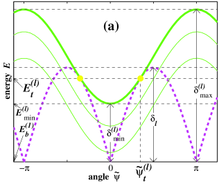
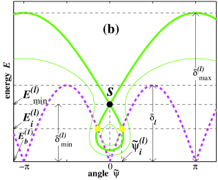
Figure 22: (Color version may be found in the online version of pre2008 as Fig. 16). A schematic figure illustrating the formation of the boundary of the lower chaotic layer for $h<h_{cr}^{(l)}(\omega_{f})$ in the ranges of $\omega_{f}$ relevant to (a) odd, and (b) even spikes. The dashed magenta line shows the GSS curve in the energy-angle plane: $E(\tilde{\psi})=E_{\rm GSS}^{(l)}(\tilde{\psi})\equiv E_{b}^{(1)}+\delta_{l}|\sin(\tilde{\psi})|$. Green lines show examples of those trajectories (98) which have points in common with the GSS curve. One of them (shown by the thick green line) relates to the formation of the upper boundary of the lower chaotic layer: in (a), the boundary is the trajectory tangent to the GSS curve; in (b), the boundary is the upper part of the separatrix generated by the saddle “$s$”. Yellow dots indicate the relevant common points of the GSS curve and the thick green line. They have angles $\pm\tilde{\psi}_{t}^{(l)}$ and energy $E_{t}^{(l)}$ in the case (a), and angles $\pm\tilde{\psi}_{i}^{(l)}$ and energy $E_{i}^{(l)}$ in the case (b). The minimum and maximum deviation of energy on the boundary from the barrier energy are denoted as $\delta_{\min}^{(l)}$ and $\delta_{\max}^{(l)}$ respectively. The maximum deviation on the GSS curve is equal to $\delta_{l}$.

It follows from the analysis carried out in the previous subsection that any state (in the $I-\tilde{\psi}$ plane) lying beyond the GSS curve but belonging to any trajectory following the equations (98) which possesses common points with the GSS curve belongs to the chaotic layer: the system starting from such a state will, sooner or later, reach the separatrix where the chaotization will necessarily occur. Therefore, the upper boundary of the chaotic layer coincides with the trajectory following equations (98) with the initial action (180) and an initial angle $\tilde{\psi}(0)$ from the range (179) such that the trajectory deviates from the barrier energy by more than does a trajectory (98)-(179)-(180) with any other initial angle. There may be only two topologically different options for such a trajectory: either it is tangent to the GSS curve, or it is the separatrix trajectory which intersects the GSS curve (some schematic examples are shown in Figs. 22(a) and 22(b) respectively; some real calculations are shown in Figs. 13 and 14).

1. Relatively small $h$

Consider first values of $h$ which are large enough for the condition (168) to be satisfied (the explicit criterion will be given in (192)) but which are smaller than the value $h_{cr}^{(l)}\equiv h_{cr}^{(l)}(\omega_{f})$ determined by Eq. (125) (its meaning is explained below). The further analysis within this range of $h$ differs for the ranges of $\omega_{f}$ relevant to odd and even spikes, and so we consider them separately.

A. Odd spikes

The relevant frequencies are:

$$\omega_{f}\approx n\omega_{m},\quad\quad n\equiv 2j-1,\quad\quad j=1,3,5,\ldots$$ (181)

Let us seek the state $\{I_{t}^{(l)},\tilde{\psi}_{t}^{(l)}\}$ (with $\tilde{\psi}_{t}^{(l)}$ within the range $]0,\pi[$) where the resonant trajectory is tangent to the GSS curve. With this aim, we equalise both the actions and the derivatives of both curves. The equality of actions immediately yields $I_{t}^{(l)}$ via $\tilde{\psi}_{t}^{(l)}$: $I_{t}^{(l)}\equiv I(E=E_{t}^{(l)})=I_{\rm GSS}^{(l)}(\tilde{\psi}_{t}^{(l)})$. The derivative along the GSS curve is obtained by differentiation of $I_{\rm GSS}^{(l)}(\tilde{\psi})$. The derivative along a resonant trajectory can be found by dividing the first dynamic equation in (14) by the second one. Substituting the expression of $I_{t}^{(l)}$ via $\tilde{\psi}_{t}^{(l)}$ into the equality of the derivatives, we obtain a closed equation for $\tilde{\psi}_{t}^{(l)}$, and its solution immediately gives us the relevant $\tilde{\psi}(0)$:

$$\left[|\epsilon^{(low)}|\cos(\tilde{\psi}_{t}^{(l)})\left(1-\frac{\omega_{f}}{n\omega(E)}-h\frac{{\rm d}q_{n}(E)}{{\rm d}E}\cos(\tilde{\psi}_{t}^{(l)})\right)+q_{n}(E)\sin(\tilde{\psi}_{t}^{(l)})\right]_{E=E_{t}^{(l)}}$$

$$=0,$$

$$E_{t}^{(l)}\equiv E_{b}^{(1)}+h|\epsilon^{(low)}|\sin(\tilde{\psi}_{t}^{(l)}),\quad\quad\tilde{\psi}_{t}^{(l)}\in[0,\pi],$$

$$n\equiv 2j-1,\quad\quad j=1,3,5,\ldots,\quad\quad\tilde{\psi}(0)=\tilde{\psi}_{t}^{(l)}.$$ (182)

A careful analysis of the phase space structure shows that, in the present case (i.e. when $h<h_{cr}^{(l)}(\omega_{f})$ while $j$ is odd), there is no separatrix of the resonant Hamiltonian (4) which would both intersect the GSS curve and possess points above the tangent trajectory. Thus, for this range of $h$, the outer boundary of the chaotic layer is formed by the trajectory following the dynamical equations (98) with the initial angle given by (183) and the initial action by (180) (Fig. 22(a)).

Let us find the lowest-order solution of Eq. (183). We neglect the term $1-\omega_{f}/(n\omega(E))$ (the result will justify this) and use the lowest-order expression for the relevant quantities: namely, Eqs. (171) and (96) for $\epsilon^{(low)}$ and $q_{n}$ respectively, and the lowest-order expression for ${\rm d}q_{n}/{\rm d}E$ which can be derived from Eq. (95):

$$\frac{{\rm d}q_{n}(E)}{{\rm d}E}=(-1)^{\left[\frac{n}{4}\right]}\frac{\pi}{4\sqrt{2}\left(E-E_{b}^{(1)}\right)\ln\left(\Phi^{-1}\right)},$$

$$n\equiv 2j-1,\quad\quad E-E_{b}^{(1)}\ll\Phi\rightarrow 0.$$ (183)

Then Eq. (183) reduces to the following equation

$$\tan^{2}(\tilde{\psi}_{t}^{(l)})=\frac{n\pi}{8\ln\left(\Phi^{-1}\right)}.$$ (184)

The lowest-order solution of (185) in the range $]0,\pi[$ is

$$\tilde{\psi}_{t}^{(l)}=(-1)^{\left[\frac{n}{4}\right]}\sqrt{\frac{n\pi}{8\ln(1/\Phi)}}+\pi\frac{1-(-1)^{\left[\frac{n}{4}\right]}}{2}.$$ (185)

It follows from the definition $E_{t}^{(l)}$ (183) and from (186) that the lowest-order expression for $E_{t}^{(l)}-E_{b}^{(1)}$ is

$$E_{t}^{(l)}-E_{b}^{(1)}=\delta_{l}\sin(\tilde{\psi}_{t}^{(l)})=\frac{\pi^{3/2}}{2}\frac{h}{\sqrt{\ln\left(1/\Phi\right)/n}}.$$ (186)

The next step is to find the minimum value of the energy on the boundary of the layer, $E_{\min}^{(l)}$. It follows from the analysis of the dynamical equations (98) that the corresponding angle $\tilde{\psi}_{\min}$ is equal to $0$ if ${\rm sign}(q_{2j-1})>0$ (i.e. $j=1,5,9,\ldots$) or to $\pi$ if ${\rm sign}(q_{2j-1})<0$ (i.e. $j=3,7,11,\ldots$): cf. Fig. 8(a). Given that the Hamiltonian (87) is constant along any trajectory (98) while the boundary coincides with one such trajectory, the values of the Hamiltonian (87) in the states $\{I(E_{\min}^{(l)}),\tilde{\psi}=\tilde{\psi}_{\min}\}$ and $\{I_{t}^{(l)},\tilde{\psi}_{t}^{(l)}\}$ should be equal to each other. In explicit form, this equality may be written as

$$\int_{E_{\min}^{(l)}}^{E_{t}^{(l)}}{\rm d}E\left(1-\frac{\omega_{f}}{n\omega(E)}\right)-h\left(q_{n}(E_{t}^{(l)})\cos(\tilde{\psi}_{t}^{(l)})-(-1)^{\left[\frac{n}{4}\right]}q_{n}(E_{\min}^{(l)})\right)=0.$$ (187)

Let us find the lowest-order solution of Eq. (188). Assume that $E_{\min}^{(l)}$ still belongs to the range of $E$ where $\omega(E)\approx\omega_{m}$ (the result will confirm this assumption). Then the integrand in (188) goes to zero in the asymptotic limit $\Phi\rightarrow 0$. Hence the integral may be neglected (again, to be justified by the result). The remaining terms in Eq. (188) should be treated very carefully. In particular, it is insufficient to use the lowest-order value (96) for $q_{n}$ since it is the difference between $q_{n}(E_{t}^{(l)})$ and $q_{n}(E_{\min}^{(l)})$ that matters. Moreover, the approximate equality $q_{n}(E_{t}^{(l)})-q_{n}(E_{\min}^{(l)})\approx{\rm d}q_{n}(E_{t}^{(l)})/{\rm d}E_{t}^{(l)}(E_{t}^{(l)}-E_{\min}^{(l)})$ does not apply here either since, as follows from Eq. (184), the derivative ${\rm d}q_{n}(E)/{\rm d}E$ may vary strongly in the range $[E_{\min}^{(l)},E_{t}^{(l)}]$ if $(E_{t}^{(l)}-E_{\min}^{(l)})/(E_{\min}^{(l)}-E_{b}^{(1)})\stackrel{{\scriptstyle\sim}}{{>}}1$ (again, to be justified by the result). That is why it is necessary to use the more accurate expression (95) for $q_{n}$. Allowing for the asymptotic expression (186) of $\tilde{\psi}_{t}^{(l)}$ and keeping only the lowest-order terms, one can finally reduce Eq. (188) to the relation

$$\ln\left(\frac{E_{t}^{(l)}-E_{b}^{(1)}}{E_{\min}^{(l)}-E_{b}^{(1)}}\right)=\frac{1}{2}.$$ (188)

Substituting here the asymptotic value of $E_{t}^{(l)}$ (187), we obtain the final lowest-order expression for the minimum deviation (along the boundary) of the energy from the barrier:

$$\delta_{\min}^{(l)}\equiv E_{\min}^{(l)}-E_{b}^{(1)}=(E_{t}^{(l)}-E_{b}^{(1)})/\sqrt{{\rm e}}=\frac{\pi^{3/2}}{2{\rm e}^{1/2}}\frac{h}{\sqrt{\ln\left(1/\Phi\right)/n}}.$$ (189)

It is necessary and sufficient that the condition $\omega(E)\approx\omega_{m}$ is satisfied at the minimal and maximal energies of the boundary to ensure that the second equality in (168) holds true, i.e. that $\omega(E)$ is close to $\omega_{m}$ for all points of the boundary.

At the minimal energy, this condition is

$$\omega_{m}-\omega(E_{b}^{(1)}+\delta_{\min}^{(l)})\ll\omega_{m}.$$ (190)

Eq. (191) determines the lower limit of the relevant range of $h$. The asymptotic form of (191) is:

$$\frac{\ln\left(\frac{\Phi\sqrt{\ln(1/\Phi)}}{h}\right)}{\ln\left(1/\Phi\right)}\ll 1.$$ (191)

We emphasize that any $h$ of the order of $h_{s0}$ (136) satisfies this condition. In the asymptotic limit $\Phi\rightarrow 0$, the left-hand part of Eq. (192) goes to zero.

As for the maximal energy, it may take values up to the energy of the lower saddle “$sl$”, i.e. $E_{sl}$ (102). Obviously, (168) is valid at this saddle, too.

B. Even spikes

The relevant frequencies are:

$$\omega_{f}\approx n\omega_{m},\quad\quad n\equiv 2j-1,\quad\quad j=2,4,6,\ldots$$ (192)

In this case, $q_{n}(E)$ and ${\rm d}q_{n}(E)/{\rm d}E$ have different signs for all $E$ within the relevant range (i.e. where $\omega(E)\approx\omega_{m}$, $q_{n}(E)\approx q_{n}(E_{m})$): cf. (96) and (184). Then, in the asymptotic limit $\Phi\rightarrow 0$, Eq. (183) for the tangency does not have any solution for $\tilde{\psi}_{t}^{(l)}$ in the relevant range. There may only be solutions very close to some of $\pi$ integers, and the corresponding energies $E_{t}^{(l)}$ are then very close to $E_{b}^{(1)}$ i.e. $\omega(E_{t}^{(l)})\ll\omega_{m}$: therefore they are irrelevant.

At the same time, unlike for the odd spikes, there exists a saddle with an angle

$$\tilde{\psi}_{s}^{(l)}=\pi\frac{1-(-1)^{\left[\frac{n}{4}\right]}}{2},$$ (193)

while the energy (which may be found as the appropriate solution of Eq. (99)) lies in the relevant vicinity of the lower barrier (Fig. 22(b)). In the lowest-order approximation, this saddle energy is:

$$E_{s}^{(l)}\equiv E_{b}^{(1)}+\delta_{s},\quad\quad\delta_{s}=\frac{\pi}{2\sqrt{2}}\frac{h}{\ln(\ln(4{\rm e}/\Phi))}\;.$$ (194)

This saddle (denoted in Fig. 22(b) as “$s$”) generates a separatrix. Its upper whiskers go to the similar adjacent saddles (shifted in $\tilde{\psi}$ by $2\pi$). In the asymptotic limit $\Phi\rightarrow 0$, the upper whiskers are much steeper than the GSS curve and hence they do not intersect it. The lower whiskers do intersect the GSS curve and, moreover, two intersections lie in the relevant energy range (Fig. 22(b)). Let us show this explicitly. We write the expression for the Hamiltonian (87) in the relevant vicinity of the barrier energy (i.e. where $\omega_{m}-\omega(E)\ll\omega_{m})$, keeping in the expression both the lowest-order terms and the terms of next order (in particular, we use Eq. (95) for $q_{n}(E)$ and take into account that $0<\sqrt{2}-nq_{n}(E)\ll\sqrt{2}$ for the relevant range of $E$):

$$\tilde{H}(I=I(E=E_{b}^{(1)}+\delta),\tilde{\psi})=-\frac{n\delta\ln\left(\frac{2\Phi}{\delta}\right)}{2\ln\left(\frac{4{\rm e}}{\Phi}\right)}+\left(\omega_{f}-\frac{n\pi}{2\ln\left(\frac{4{\rm e}}{\Phi}\right)}\right)\frac{2\Phi}{\pi}\ln\left(\frac{4{\rm e}}{\Phi}\right)-$$

$$-(-1)^{\left[\frac{n}{4}\right]}h\sqrt{2}\left(1+\frac{n\pi\ln\left(\frac{2\Phi}{\delta}\right)}{8\ln\left(\frac{4{\rm e}}{\Phi}\right)}\right)\cos(\tilde{\psi}),$$

$$\omega_{m}-\omega(E+\delta)\ll\omega_{m}.$$ (195)

The Hamiltonian $\tilde{H}$ should possess equal values at the saddle “$s$” and at the intersections of the separatrix and the GSS curve. Let us denote the angle of the intersection in the range $]0,\pi[$ as $\tilde{\psi}_{i}^{(l)}$, and let us denote the deviation of its energy $E_{i}^{(l)}$ from $E_{b}^{(1)}$ as $\delta_{i}^{(l)}\equiv\delta_{l}\sin(\tilde{\psi}_{i}^{(l)})$.

Assuming that $|\tilde{\psi}_{i}^{(l)}-\tilde{\psi}_{s}^{(l)}|\ll 1$ (the result will confirm this) so that

$$\cos(\tilde{\psi}_{i}^{(l)})\approx(-1)^{[n/4]}(1-(\tilde{\psi}_{i}^{(l)}-\tilde{\psi}_{s}^{(l)})^{2}/2)\approx$$

$$\approx(-1)^{[n/4]}(1-(\delta_{i}^{(l)}/\delta_{l})^{2}/2)\approx(-1)^{[n/4]}(1-(\delta_{i}^{(l)}/h)^{2}/4),$$

the equality of the values of $\tilde{H}$ is:

$$\frac{n}{2\ln\left(\frac{4{\rm e}}{\Phi}\right)}\left(\delta_{s}\ln\left(\frac{2\Phi}{\delta_{s}}\right)-\delta_{i}^{(l)}\ln\left(\frac{2\Phi}{\delta_{i}^{(l)}}\right)\right)=h\sqrt{2}\frac{n\pi}{8}\frac{\ln\left(\frac{\delta_{s}}{\delta_{i}^{(l)}}\right)}{\ln\left(\frac{4{\rm e}}{\Phi}\right)}-\frac{(\delta_{i}^{(l)})^{2}}{2\sqrt{2}h}.$$ (196)

Let us assume that, in the asymptotic limit $\Phi\rightarrow 0$, $\delta_{i}^{(l)}\ll\delta_{s}$ (the result will confirm this). Then the left-hand part is asymptotically smaller than the first term in the right-hand part. So, Eq. (197) implies, in the asymptotic limit, that the right-hand side equals zero. Expressing $h$ via $\delta_{s}$ from Eq. (195), we finally obtain a closed transcendental equation for $\delta_{s}/\delta_{i}^{(l)}$:

$$\left(\frac{\delta_{s}}{\delta_{i}^{(l)}}\right)^{2}\ln\left(\frac{\delta_{s}}{\delta_{i}^{(l)}}\right)=\frac{\pi\ln\left(\frac{4{\rm e}}{\Phi}\right)}{n\left(\ln\left(\ln\left(\frac{4{\rm e}}{\Phi}\right)\right)\right)^{2}}\equiv A.$$ (197)

In the asymptotic limit $\Phi\rightarrow 0$, the quantity $A$ diverges and, hence, the lowest-order asymptotic solution of Eq. (198) reads as

$$\frac{\delta_{s}}{\delta_{i}^{(l)}}=\sqrt{\frac{2A}{\ln(A)}}.$$ (198)

Substituting here the expression (195) for $\delta_{s}$ and the expression (198) for $A$, we obtain:

$$\delta_{i}^{(l)}=h\frac{1}{4}\sqrt{\frac{n\pi\ln\left(\ln\left(\frac{4{\rm e}}{\Phi}\right)\right)}{\ln\left(\frac{4{\rm e}}{\Phi}\right)}}.$$ (199)

Thus, we have proved the following asymptotic properties of the separatrix generated by the saddle “$s$”: (i) the lower whiskers of the separatrix do intersect the GSS curve in the relevant range of $E$ (i.e. where the resonant approximation is valid); and (ii) the upper whiskers of the separatrix do not intersect the GSS curve (there is no solution of Eq. (197) in the range $\delta_{i}^{(l)}>\delta_{s}$). The former property confirms the self-consistency of the asymptotic theory for even spikes; the latter property means that the upper outer boundary of the lower chaotic layer is formed by the upper whiskers of the separatrix generated by the saddle “$s$”.

Finally, we note explicitly that the minimal (along the boundary) deviation of energy from the barrier energy occurs exactly at the saddle “$s$”, i.e.

$$\delta_{\min}^{(l)}=\delta_{s}.$$ (200)

2. Relatively large $h$.

As $h$ grows, the boundary of the layer rises while the lower part of the resonance separatrix, on the contrary, falls. They reconnect at the critical value of $h$, $h_{cr}^{(l)}\equiv h_{cr}^{(l)}(\omega_{f})$, determined by Eq. (125), which may be considered as the absorption of the resonance by the chaotic layer. If $h$ grows further, then the GSS curve and the resonance separatrix intersect. As a result, the trajectory starting from the state of angle (183) and action (180), for odd spikes, or from the saddle “$s$”, for even spikes, is encompassed by the resonance separatrix. So, it no longer forms the outer boundary of the layer. Rather it forms the inner boundary i.e. the boundary of the main island of stability inside the layer, repeated periodically in $\tilde{\psi}$ with a period $2\pi$ (cf. analogous islands in the upper layer in Fig. 13). Unless the lower chaotic layer reconnects with the upper one, the outer boundary of the lower layer is formed by the upper part of the resonance separatrix. The relevant initial angle $\tilde{\psi}(0)$ on the GSS curve corresponds to the intersection of the GSS curve with the resonance separatrix (cf. the analogous situation for the upper layer in Fig. 13).

7.2 Upper chaotic layer

The upper chaotic layer may be treated analogously to the lower layer. We present here only the results.

Similarly to the lower-layer case, one may consider the ranges of relatively small $h$ (namely, smaller than $h_{cr}^{(u)}\equiv h_{cr}^{(u)}(\omega_{f})$ determined by Eq. (126)) and relatively large $h$ (i.e. $h>h_{cr}^{(u)}$). In the former range, the formation of the boundary occurs in a manner which is, in a sense, opposite to that for the lower-layer case. For even spikes, the lower outer boundary is formed by tangency while, for odd spikes, it is formed by the lower part of the separatrix generated by the saddle “$\tilde{s}$”, analogous to the saddle “$s$”in the lower-layer case.

So, for even spikes, the angle of tangency $\tilde{\psi}_{t}^{(u)}$ is determined by:

$$\left[|\epsilon^{(up)}|\cos(\tilde{\psi}_{t}^{(u)})\left(1-\frac{\omega_{f}}{n\omega(E)}-h\frac{{\rm d}q_{n}(E)}{{\rm d}E}\cos(\tilde{\psi}_{t}^{(u)})\right)-q_{n}(E)\sin(\tilde{\psi}_{t}^{(u)})\right]_{E=E_{t}^{(u)}}$$

$$=0,$$

$$E_{t}^{(u)}\equiv E_{b}^{(2)}-h|\epsilon^{(up)}|\sin(\tilde{\psi}_{t}^{(u)})\quad\quad\tilde{\psi}_{t}^{(u)}\in\left[0,\pi\right],$$

$$n\equiv 2j-1,\quad\quad j=2,4,6,\ldots,\quad\quad\tilde{\psi}(0)=\tilde{\psi}_{t}^{(u)},$$ (201)

and $\tilde{\psi}_{t}^{(u)}$ determines the tangency energy:

$$E_{t}^{(u)}=E_{b}^{(2)}-h|\epsilon^{(up)}|\sin(\tilde{\psi}_{t}^{(u)}),$$ (202)

where the quantity $\epsilon^{(up)}$ is described by the formula

$$\epsilon^{(up)}(\omega_{f})=2\int_{0}^{\infty}{\rm d}t\;\dot{q}_{s}^{(up)}(t)\cos(\omega_{f}t)\,,$$ (203)

where $\dot{q}_{s}^{(up)}(t)$ is the time dependence of the velocity along the separatrix associated with the upper barrier and the instant $t=0$ is chosen so that $q_{s}^{(up)}(t=0)$ is equal to the coordinate of the lower barrier while $\dot{q}_{s}^{(up)}>0$ for $t\in[0,\infty[$. The dependence $\left|\epsilon^{(up)}(\omega_{f})\right|$ in Eq. (204) is shown for $\Phi=0.2$ in Fig. 21(b).

The asymptotic form of Eq. (204) is

$$\epsilon^{(up)}\equiv\epsilon^{(up)}(\omega_{f})=2\pi\cos\left(\frac{\pi\omega_{f}}{4\omega_{m}}\right)\,.$$ (204)

For $\omega_{f}=\omega_{s}^{(j)}\approx(2j-1)\omega_{m}$, Eq. (204) reduces to

$$\epsilon^{(up)}(\omega_{s}^{(j)})\approx 2\pi\cos\left((2j-1)\frac{\pi}{4}\right)=\sqrt{2}\pi(-1)^{\left[\frac{2j+1}{4}\right]},$$

$$j=1,2,3,...,\quad\Phi\rightarrow 0.$$ (205)

The lowest-order solution of (202) is given in Eq. (121), so that $E_{t}^{(u)}$ is approximated by Eq. (122). The maximal energy on the lower boundary of the layer corresponds to $\tilde{\psi}(t)=\pi$ if $j=2,6,10,\ldots$ or $0$ if $j=4,8,12,\ldots$ and is determined by Eq. (123). The asymptotic value of the minimal deviation from the upper barrier of the energy at the boundary, $\delta_{\min}^{(u)}$, is given in Eq. (124).

For odd spikes, the boundary is formed by the lower part of the separatrix generated by the saddle “$\tilde{s}$ ”. The angle of the saddle is given in Eq. (117) while the deviation of its energy from the barrier is approximated in lowest-order by Eq. (118).

As $h$ grows, the boundary of the layer falls while the upper part of the upper resonance separatrix rises. They reconnect at $h=h_{cr}^{(u)}\equiv h_{cr}^{(u)}(\omega_{f})$, as determined by Eq. (126), which may be considered as the absorption of the resonance by the layer.

For larger $h$, the boundary of the layer is formed by the lower part of the upper resonance separatrix (Fig. 13), unless the latter intersects the lower GSS curve (in which case, $h_{cr}^{(u)}$ marks the onset of global chaos).

References

- (1) Abdullaev S.S.: Construction of Mappings for Hamiltonian Systems and Their Applications. Springer, Berlin, Heidelberg (2006).
- (2) Abramovitz M., Stegun I.: Handbook of Mathematical Functions. Dover, New York (1970).
- (3) Andronov A.A., Vitt A.A., Khaikin S.E.: Theory of Oscillators. Pergamon, Oxford (1966).
- (4) Arnold V.I.: Instability of dynamical systems with several degrees of freedom. Sov. Math. Dokl. 5, 581–585 (1964).
- (5) Bogolyubov N.N., Mitropolsky Yu.A.: Asymptotic Methods in the Theory of Nonlinear Oscillators. Gordon and Breach, New York (1961).
- (6) Carmona H.A. et al.: Two dimensional electrons in a lateral magnetic superlattice. Phys. Rev. Lett. 74, 3009–3012 (1995).
- (7) Chernikov A.A. et al.: Minimal chaos and stochastic webs. Nature 326, 559–563 (1987).
- (8) Chernikov A.A. et al.: Some peculiarities of stochastic layer and stochastic web formation. Phys. Lett. A 122, 39–46 (1987).
- (9) Chernikov A.A. et al.: Strong changing of adiabatic invariants, KAM-tori and web-tori. Phys. Lett. A 129, 377–380 (1988).
- (10) Chirikov B.V.: A universal instability of many-dimensional oscillator systems. Phys. Rep. 52, 263–379 (1979).
- (11) del-Castillo-Negrete D., Greene J.M., Morrison P.J.: Area-preserving non-twist maps: periodic orbits and transition to chaos. Physica D 61, 1–23 (1996).
- (12) Dullin H.R., Meiss J.D., Sterling D.: Generic twistless bifurcations. Nonlinearity 13, 203–224 (2000).
- (13) Dykman M.I., Soskin S.M., Krivoglaz M.A.: Spectral distribution of a nonlinear oscillator performing Brownian motion in a double-well potential. Physica A 133, 53–73 (1985).
- (14) Elskens Y. and Escande D.F.: Slowly pulsating separatrices sweep homoclinic tangles where islands must be small: an extension of classical adiabatic theory. Nonlinearity 4, 615–667 (1991).
- (15) Fromhold T.M. et al.: Effects of stochastic webs on chaotic electron transport in semiconductor superlattices. Phys. Rev. Lett. 87, 046803-1–046803-4 (2001).
- (16) Fromhold T.M. et al.: Chaotic electron diffusion through stochastic webs enhances current flow in superlattices. Nature 428, 726–730 (2004).
- (17) Gelfreich V., private communication.
- (18) Gelfreich V.G., Lazutkin V.F.: Splitting of separatrices: perturbation theory and exponential smallness. Russian Math. Surveys 56, 499–558 (2001).
- (19) Howard J.E. and Hohs S.M.: Stochasticity and reconnection in Hamiltonian systems. Phys. Rev. A 29, 418–421 (1984).
- (20) Howard J.E. and Humpherys J.: Non-monotonic twist maps. Physica D 80, 256–276 (1995).
- (21) Landau L.D. and Lifshitz E.M.: Mechanics. Pergamon, London (1976).
- (22) Leonel E.D.: Corrugated Waveguide under Scaling Investigation. Phys. Rev. Lett. 98, 114102-1–114102-4 (2007).
- (23) Lichtenberg A.J. and Lieberman M.A.: Regular and Stochastic Motion. Springer, New York (1992).
- (24) Luo A.C.J.: Nonlinear dynamics theory of stochastic layers in Hamiltonian systems. Appl. Mech. Rev. 57, 161–172 (2004).
- (25) Luo A.C.J., Gu K., Han R.P.S.: Resonant-Separatrix Webs in Stochastic Layers of the Twin-Well Duffing Oscillator. Nonlinear Dyn. 19, 37–48 (1999).
- (26) Morozov A.D.: Degenerate resonances in Hamiltonian systems with 3/2 degrees of freedom. Chaos 12, 539–548 (2002).
- (27) Neishtadt A.I.: Change in adiabatic invariant at a separatrix. Sov. J. Plasma Phys. 12, 568–573 (1986).
- (28) Neishtadt A.I., Sidorenko V.V., and Treschev D.V.: Stable periodic motions in the problem on passage trough a separatrix. Chaos 7, 2–11 (1997).
- (29) Piftankin G.N., Treschev D.V.: Separatrix maps in Hamiltonian systems. Russian Math. Surveys 62, 219–322 (2007).
- (30) Prants S.V., Budyansky M.V., Uleysky M.Yu., Zaslavsky G.M.: Chaotic mixing and transport in a meandering jet flow. Chaos 16, 033117-1–033117-8 (2006).
- (31) Rom-Kedar V.: Transport rates of a class of two-dimensional maps and flows. Physica D 43, 229–268 (1990).
- (32) Rom-Kedar V.: Homoclinic tangles – classification and applications. Nonlinearity 7, 441–473 (1994).
- (33) Schmelcher P. and Shepelyansky D.L.: Chaotic and ballistic dynamics for two–dimensional electrons in periodic magnetic fields. Phys. Rev. B 49, 7418–7423 (1994).
- (34) Shevchenko I.I.: Marginal resonances and intermittent Behavious in the motion in the vicinity of a separatrix. Phys. Scr. 57, 185–191 (1998).
- (35) Shevchenko I.I.: The width of a chaotic layer. Phys. Lett. A 372, 808–816 (2008).
- (36) Schmidt G.J.O.: Deterministic diffusion and magnetotransport in periodically modulated magnetic fields. Phys. Rev. B 47, 13007–13010 (1993).
- (37) Soskin S.M., unpublished.
- (38) Soskin S.M. and Mannella R.: New Approach To The Treatment Of Separatrix Chaos. In: Proceedings of the ICNF-2009. In press.
- (39) Soskin S.M., Mannella R.: Maximal width of the separatrix chaotic layer. Submitted to Phys. Rev. E.
- (40) Soskin S.M., Mannella R., Arrayás M. and Silchenko A.N.: Strong enhancement of noise-induced escape by transient chaos. Phys. Rev. E 63, 051111-1–051111-6 (2001).
- (41) Soskin S.M., Mannella R. and McClintock P.V.E.: Zero-Dispersion Phenomena in oscillatory systems. Phys. Rep. 373, 247–409 (2003).
- (42) Soskin S.M., Yevtushenko O.M., Mannella R.: Divergence of the Chaotic Layer Width and Strong Acceleration of the Spatial Chaotic Transport in Periodic Systems Driven by an Adiabatic ac Force. Phys. Rev. Lett. 95, 224101-1–224101-4 (2005).
- (43) Soskin S.M., Mannella R., Yevtushenko O.M.: Matching of separatrix map and resonant dynamics, with application to global chaos onset between separatrices. Phys. Rev. E 77, 036221-1–036221-29 (2008).
- (44) Soskin S.M., Mannella R., Yevtushenko O.M.: Separatrix chaos: new approach to the theoretical treatment. In: Chandre C., Leoncini X., and Zaslavsky G. (eds.) Chaos, Complexity and Transport: Theory and Applications (Proceedings of the CCT-07), pp. 119-128. World Scientific, Singapore, (2008).
- (45) Soskin S.M., Yevtushenko O.M., Mannella R.: Adiabatic divergence of the chaotic layer width and acceleration of chaotic and noise-induced transport. Commun. Nonlinear Sci. Numer. Simulat. In press, doi:10.1016/j.cnsns.2008.06.025.
- (46) Soskin S.M., Khovanov I.A., Mannella R., McClintock P.V.E.: Enlargement of a low-dimensional stochastic web. In: Proceedings of the ICNF-2009. In press.
- (47) Vecheslavov V.V.: Chaotic layer of a pendulum under low-and medium-frequency perturbations. Tech. Phys. 49, 521–525 (2004).
- (48) Ye P.D. et al.: Electrons in a periodic magnetic field induced by a regular array of micromagnets. Phys. Rev. Lett. 74, 3013-3016 (1995).
- (49) Yevtushenko O.M. and Richter K.: Effect of an ac electric field on chaotic electronic transport in a magnetic superlattice. Phys. Rev. B 57, 14839–14842 (1998).
- (50) Yevtushenko O.M. and Richter K.: AC-driven anomalous stochastic diffusion and chaotic transport in magnetic superlattices. Physica E 4, 256–276 (1999).
- (51) Zaslavsky G.M.: Physics of Chaos in Hamiltonian systems, 2nd edn. Imperial Colledge Press, London (2007).
- (52) Zaslavsky G.M.: Hamiltonian Chaos and Fractional Dynamics. Oxford University Press, Oxford (2008).
- (53) Zaslavsky G.M. and Filonenko N.N.: Stochastic instability of trapped particles and conditions of application of the quasi-linear approximation. Sov. Phys. JETP 27, 851–857 (1968).
- (54) Zaslavsky G.M. et al.: Stochastic web and diffusion of particles in a magnetic field. Sov. Phys. JETP 64, 294–303 (1986).
- (55) Zaslavsky G.M., Sagdeev R.D., Usikov D.A. and Chernikov A.A.: Weak Chaos and Quasi-Regular Patterns. Cambridge University Press, Cambridge (1991).