Measuring Measurement: Theory and Practice

Abstract

Recent efforts have applied quantum tomography techniques to the calibration and characterization of complex quantum detectors using minimal assumptions. In this work we provide detail and insight concerning the formalism, the experimental and theoretical challenges and the scope of these tomographical tools. Our focus is on the detection of photons with avalanche photodiodes and photon number resolving detectors and our approach is to fully characterize the quantum operators describing these detectors with a minimal set of well specified assumptions. The formalism is completely general and can be applied to a wide range of detectors.

I Introduction

The quantum properties of nature reveal themselves only to carefully designed measurement techniques Resch ; Pryde . In addition, most quantum information applications both computational and cryptographic, rely on a certain knowledge of the measurement apparatuses involved. Indeed for these protocols we often need to ensure that we associate detector outcomes with the correct quantum mechanical operation or quantum state. More critically, the assumption of a fully characterized detector completely underlies both quantum state tomography (QST) and quantum process tomography (QPT) PhysRevLett.70.1244 ; PhysRevLett.78.390 ; kwiat . State tomography has become an important tool for characterizing states, partially due to the realization that non-classical states are a resource for performing tasks such as enhanced precision metrology, quantum communication, and quantum computation. Often taken for granted, measurement also plays a crucial role in these tasks and in some can even eliminate the need for entanglement. In enhanced precision metrology, appropriate measurements alone can give rise to super-resolution Resch and Heisenberg-limited sensitivity Pryde . In communication, measurement allows entanglement swapping, and thus, is central to quantum repeaters. And for computing, measurement based schemes enable quantum computation Raussendorf ; Raussendorf-Briegel-prl . It follows that measurement should also be considered a resource for quantum protocols. In QST a given number of measurements on many copies of an unknown state reveal its density operator PhysRevA.40.2847 ; PhysRevLett.70.1244 ; PhysRevA.60.674 . Characterising the operators that govern an evolution or a channel – QPT – amounts to applying the process to a set of input states, and subsequently fully characterising the output states chuang-1996 ; PhysRevLett.78.390 ; PhysRevLett.80.5465 ; kwiat ; lvovsky-2008 . In this paper we study quantum detector tomography (QDT) PRLSoto ; dariano-2004-93 ; PhysRevA.64.024102 ; JMOTomo ; NaturePhysTomo , in which a detector’s outcome statistics in response to a set of input states determine the operators that describe that detector. State and detector tomography evidently exhibit a dual role: Either the input is well-known and the detector is to be characterised, or the detector is well-known and the state is to be tomographically reconstructed.

Throughout the paper, we focus on examples from optics. However, quantum detector tomography is a general concept, applicable to any quantum detector. Building upon previous theoretical descriptions PRLSoto ; dariano-2004-93 ; PhysRevA.64.024102 ; JMOTomo we will introduce the concept of detector tomography in the next section. Alongside, we will present examples detailing the reconstruction of simple detectors to introduce the key concepts. Subsequently, based on recent experiments NaturePhysTomo we will present the methods used in optical detector tomography and the convex optimization methods Convex which allow an efficient and simple numerical optimization. Finally, in the last section, we will discuss some of the theoretical and experimental challenges involved and how to address them.

II Detector tomography

II.1 Definitions

In quantum mechanics, the operator describing a measurement apparatus is, in its most general form, a positive operator valued measure (POVM). The POVM elements $\{\pi_{n}\}$ describe the possible outcomes, labeled here by $n$. Particularly, for a projective measurement, the POVM elements are orthogonal and simplify to the familiar form

$$\pi_{n}=|\psi_{n}\rangle\langle\psi_{n}|.$$

In quantum optics, an example of a POVM that consists of projectors is that of an eight-port homodyne, $\{|\alpha\rangle\langle\alpha|:\alpha\in\mathbbm{C}\}$.

Now, given an input state $\rho$, the probability $p_{\rho,n}$ of obtaining output $n$ is

$$p_{\rho,n}=\mathop{\rm Tr}{}\left(\rho\pi_{n}\right).$$ (1)

It follows that the POVM elements must be positive semi-definite, $\pi_{n}\geq 0$, while observing

$$\sum_{n}\pi_{n}=\mathbbm{1},$$ (2)

if we want probabilities adding up to one. Inverting Eq. (1) to extract $\pi_{n}$ subject to the aforementioned conditions is the task behind detector tomography.

II.2 Assumptions

Detector tomography raises fundamental questions about the kind of information we can extract from Nature. It is reasonable to think that state tomography performed with poorly characterized detectors can lead to unwanted errors. In addition, for quantum cryptography, a mischaracterization of states or detectors may lead to channels through which an eavesdropper may attack invalidating certain security proofs (see for ex. Makarov ). Indeed, if we misjudge the noise level, then we misjudge the information the eavesdropper possesses. Interestingly, quantum key distribution with totally uncharacterized detectors is possible in principle, based entirely on correlations violating Bell’s inequalities, but at the expense of having much smaller rates Masanes1 ; Masanes2 . An in depth discussion of our assumptions is therefore necessary to avoid unwanted errors in our detector estimation.

Generally, there are going to be assumptions about the input states produced by the source. In the reconstruction, we will often need to assume we can truncate an infinite dimensional Hilbert space, such as in the case of photon number. On the detector side, a common assumption will be that the detector is memory-less: the previous measurements do not modify the result of future measurements. For example, this assumption fails when detector deadtimes are longer than the time between consecutive measurements. All of these assumptions need to be tested.

More generally, we can ask what the working minimal set of assumptions happens to be. An assumption-free tomography could use a complete black box approach: prepare a collection of unknown states, measure them and try to draw some conclusions about both the detector and the states. Specifically, we could have some classical controls to prepare quantum states $\{\rho_{\lambda}\}$ characterized by the index $\lambda$ and some classical pointer to indicate the possible outcomes, labeled $n$. Minimizing the set of assumptions would constrain us to draw our conclusions exclusively from the joint probability distribution $\{p_{\lambda,n}\}$.

To further constrain the problem we can add the standard assumptions: An underlying Hilbert space of fixed dimension, normalized positive density matrices and positive POVM elements $\{\pi_{n}\}$ satisfying $\sum_{n=1}^{N}\pi_{n}=\mathbbm{1}$. However, without further assumptions, the relationship between $\lambda$ and $\rho$’s $d^{2}-1$ parameters is completely unknown, as is that between $n$ and $\{\pi_{n}\}$’s $(N-1)d^{2}$ parameters.

This discussion highlights the inherent difficulties that a fully general inference (or tomographic) scheme entails. Reasonable assumptions are thus needed but the question of general tomography remains an interesting one to be explored. In this direction, some progress has been made in self-testing maps. In this context states are prepared with classical recipes and families of unitary gates are revealed with few assumptions about the quantum states (however known measurements in the computational basis are required) self-testing .

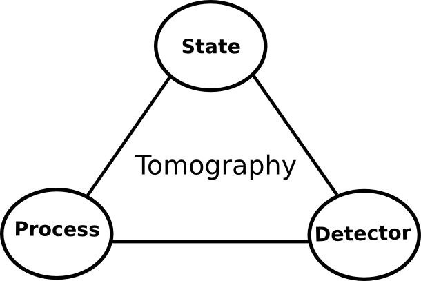
Figure 1: It is generally possible to divide an experiment into preparation, evolution, and measurement. However, if one corner in the above diagram is unknown or missing, then we need assumptions about the other two.

As shown diagramatically in Fig.  1 we can divide any experiment into preparation, evolution and measurement. If one of the elements of the triad is unknown or missing then we need to previously characterize the other two making assumptions in the process.

II.3 Practical detector tomography

In state tomography, one must perform a set of measurements $\{\pi_{n}\}$ spanning the space of the density operator to be reconstructed. If the state is defined on a $d$-dimensional Hilbert space, then it will be fully specified by $d^{2}-1$ real parameters (respecting the constraint of unit trace). To fully characterize a quantum detector, we need the data obtained from measuring input states from a well-characterized source. To recover all the POVM elements $\{\pi_{n}\}$ from the measured statistics $p_{\rho,n}$ the probe states or input states must also be chosen to form a set $\{\rho_{j}\}$ that is tomographically complete: the span of the operators $\{\rho_{j}\}$ – which are not necessarily linearly independent – must be the entire space from which $\pi_{n}$ is taken. A spanning set forming an operator basis will have at least $d^{2}(k-1)$ elements for a $k$ outcome detector. In principle this is sufficient to calculate the direct inversion of Eq. (1). However experimental detector tomography carries additional requirements. Clearly the probe states should be previously characterised, and large numbers of them should be easily and reliably generated. In the case of optical detectors, coherent states are ideal candidates since a laser can generate them directly and we can create a tomographically complete set by transforming their amplitude through attenuation (for example with a beam splitter) and a phase-shifter (an optical path delay). Using input states $\{|\alpha\rangle\langle\alpha|:\alpha\in\mathbbm{C}\}$ one can then reconstruct the $Q$-function of the detector PRLSoto which is simply proportional to the measured statistics,

$$p_{\alpha,n}=\frac{1}{\pi^{2}}\langle\alpha|\pi_{n}|\alpha\rangle=\frac{1}{\pi}Q_{n}(\alpha).$$ (3)

Since $Q_{n}(\alpha)$ of each POVM contains the same information as the element $\pi_{n}$ itself, predictions of the detection probabilities for arbitrary input states can then be calculated directly from the Q-function.

II.4 Simple example: the perfect photocounter

Consider as a simple example the case of a perfect photon number detector This projective measurement is characterized by its POVM elements, $\left\{\pi_{n}=|n\rangle\langle n|:{n=0,\dots,N}\right\}$. In the simplest of scenarios, using pure number states, $\left\{\rho=|m\rangle\langle m|:{m=0,\dots,N}\right\}$, the characterization would be trivial, since the statistics

$$p_{\rho,n}=\delta_{n,m}$$

would immediately characterize our detector. From a more practical perspective, pure number states are very hard to generate, especially for high photon numbers. Using coherent states is therefore a more realistic approach. Assuming a collection $\{|\alpha_{i}\rangle:i=1,\dots,D\}$ of perfect coherent states our statistics would then become

$$p_{\alpha_{i},n} =\mathop{\rm Tr}{}\left(|\alpha_{i}\rangle\langle\alpha_{i}|n\rangle\langle n|\right)$$

$$=e^{-{|\alpha_{i}|}^{2}/2}\frac{|\alpha_{i}|^{2n}}{n!}.$$

Of course in an experiment we would not know the POVM elements in advance, and we would need to express them with a generic expression such as

$$\pi_{n}=\sum_{k,p}\theta_{k,p}^{(n)}|k\rangle\langle p|$$

suffering only the constraint $0\leq\pi_{n}\leq\mathbbm{1}$. Fortunately, these operators can be simplified: interposing a phase shifter in the coherent beam’s path we can check if the statistics are independent of the phase. If they are we can infer the phase independence of the POVM. Our operators then become $\pi_{n}=\sum_{k}\theta_{k}^{(n)}|k\rangle\langle k|$ and the statistics can be expressed as

$$p_{\alpha_{i},n}=e^{-{|\alpha_{i}|}^{2}/2}\sum_{k=0}^{\infty}\frac{|\alpha_{i}|^{2k}}{k!}\theta_{k}^{(n)}.$$ (4)

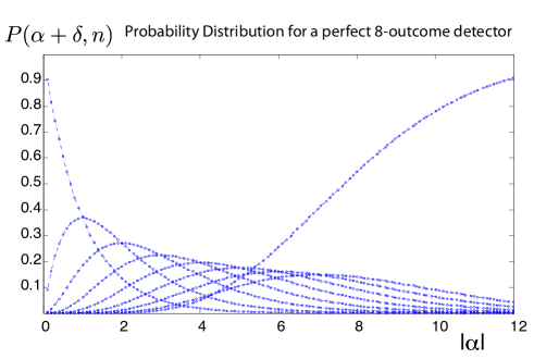
Figure 2: Outcome probability distributions for an $8$-outcome detector. Each curve represents the probability of that outcome (zero clicks, one click, etc) happening vs. the value of the intensity of the coherent state arriving at the detector.

For a perfect photon number detector that can discriminate up to eight photons, the outcome probability distributions would be the one shown in Fig. 2.

We now consider how one would estimate the POVM elements from these probability distributions, which form a set of simple simulated data. Our goal is to invert Eq. (4). To do so we can write a matrix version of the equation. Given the set of coherent states $\{\alpha_{1},\dots,\alpha_{D}\}$, and truncating the number states at a sufficiently large $M$, we can write

$${P}={F}{\Pi}.$$ (5)

Here, we have taken

$$p_{\alpha_{i},n}= \langle\alpha_{i}|\hat{\pi}_{n}|\alpha_{i}\rangle$$

$$=\langle\alpha_{i}|\biggl{(}\sum_{k=0}^{M}\theta_{k}^{(n)}|k\rangle\langle k|\biggr{)}|\alpha_{i}\rangle$$

$$=e^{-|\alpha_{i}|^{2}}\sum_{k=0}^{M}\frac{|\alpha_{i}|^{2k}}{k!}\theta_{k}^{(n)}$$

$$=\sum_{k=0}^{M}F_{k}(\alpha_{i})\theta_{k}^{(n)}$$

$$=\sum_{k=0}^{M}{F}_{i,k}{\Pi}_{k,n}.$$

So the matrix $P$ has entries

$$P_{i,n}=p_{\alpha_{i},n},$$

$F$ entries ${F}_{i,k}=F_{k}(\alpha_{i})$, and $\Pi$ entries ${\Pi}_{k,n}=\theta_{k}^{(n)}$. For an $N$-outcome detector, this gives the matrix dimensions of $P\in\mathbbm{C}^{D\times N}$, $F\in\mathbbm{C}^{D\times M}$, and $\Pi\in\mathbbm{C}^{M\times N}$.

Now, to obtain $\Pi$, we can simply solve the convex optimization problem

min $$\left\{\|{P}-F\Pi\|_{2}\right\},$$

subject to $$\;\pi_{n}\geq 0,\,\;\;\sum_{n=1}^{N}\pi_{n}=\mathbbm{1}.$$ (6)

This is a convex problem, because the norm $\|.\|_{2}$, defined as $\|A\|_{2}=(\sum_{i,j}|A_{i,j}|^{2})^{1/2}$ for matrix $A$ is a convex function and the positivity constraint $\pi_{n}\geq 0$ is semi-definite. The result of a single such minimization is shown in Fig. 3, where we recover the expected POVM elements

$$\biggl{\{}|0\rangle\langle 0|,|1\rangle\langle 1|,,\dots,.,|7\rangle\langle 7|,\mathbbm{1}-\sum_{k=0,\dots,8}|k\rangle\langle k|\biggr{\}}.$$ (7)

It is remarkable that even introducing some statistical noise in the simulated data the results are just as perfect. Indeed, if instead of using $p_{\alpha_{i},n}=\mathop{\rm Tr}{}\left(|\alpha_{i}\rangle\langle\alpha_{i}|n\rangle\langle n|\right)$ we use, $p_{\alpha_{i},n}=\mathop{\rm Tr}{}\left(|\alpha_{i}+\delta_{i}\rangle\langle\alpha_{i}+\delta_{i}|n\rangle\langle n|\right)$ where $\{\delta_{i}\}$ represent a $2$% random noise, then the results are just as robust as without. This will be discussed in more detail in later sections as it relates to the technical noise of the laser. Let us then move on to more realistic detectors and see the problems that loss and finite photon resolution introduce.

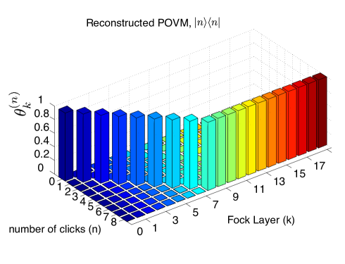
Figure 3: Reconstructed POVM of a theoretical photon number detector with $9$ bins. The POVM elements, $\pi_{n}=\sum_{k}\theta_{k}^{(n)}|k\rangle\langle k|$, are the result of the optimization in Eq. (II.4), and show a perfect result even though a $2$% random noise was added to the data (changing the value of the coherent state amplitudes).

III Why detector tomography?

In spite of its first sucessful applications, one could question the need for detector tomography. After all, detectors have been calibrated in the past without tomographic techniques. However, as quantum technology makes striking advances, quantum detectors are becoming more complex and, thus, susceptible to imperfections that are not incorporated in the bottom-up approach of modelling. In contrast, with tomography one can design detectors with a top-down aproach by fully characterizing the final detector operation. For example, photo-detection has seen the advent of single-carbon-nanotube detectors nanotube-detector , charge integration photon detectors (CIPD) CIDP , Visible Light Photon Counters (VLPC) VLPC , quantum dot arrays shields:3673 , superconducting edge and picosecond sensors miller:791 ; super-pico or time multiplexing detectors based on commercial Si-APDs loopy ; loopy0 . Certainly understanding and modelling in full detail the noise, loss and coherence characteristics of these technologies is far from trivial. Detector tomography is an answer to those challenges and, additionally, will allow us to benchmark competing detectors. Such characterized detectors also allow for the preparation of non-Gaussian states in a certified manner, such as photon subtracted states. Hence, such detectors are readily useable in protocols such as entanglement distillation based on non-Gaussian states Dis1 ; Dis ; Dis2 , in schemes increasing entanglement by means of photon subtraction In , enhancing the teleportation fidelity Tel1 ; Tel2 , or in other applications of non-Gaussian states Loophole ; Met , specifically in the context of quantum metrology.

Let us discuss more precisely how detector tomography can provide an advantage with respect to traditional calibration methods.

III.1 The limits of calibration

Standard calibration methods require a model of the detector. The parameters of this model are then estimated experimentally using states and standard assumptions. However, for specific applications, this models can become very complicated with a daunting number of parameters. For example, a detector as simple as a Yes/No avalanche photo diode (APD) becomes very hard to model when all noise sources are studied migdall1 ; migdall2 . Tomography sidesteps this by enabling the operational detector to be measured directly. Another advantage can be to avoid errors or pitfalls from standard calibration. An example is the use of Bell-state detectors which can appear to be working while frequency correlations in the input states obscure the results Broken-Bell-State-Detector ; Ian_royal_soc . To avoid such pitfalls detectors are often used in the rages where their behaviour is easily calibrated. Detector tomography could extend the range of applicability of existing detectors and help design more complicated ones. Let us now look at other advantages of full detector tomography.

III.2 Quantitative entanglement verification

Once a detector is fully characterized, it can be used to characterize states in a certified fashion. In this respect, a detector is still useful if it is imperfect in the sense that its POVM elements are not just unit rank projections: One can use them in an estimation problem, or in a setting that unambiguously estimates properties of a state. This is one of the key applications of detector tomography, in that imperfect devices can be used to very reliably perform estimation. A specifically important example is the direct detection of entanglement: Once detectors are characterized, one can perform measurements and then find lower bounds to entanglement measures, based on these measurements. This is an idea presented in Ref. Auden (see also Refs. Quant ; GuehneShort ; GuehneLong ; Wunder-Plenio ). Here we discuss the specific issues related to infinite-dimensional systems and photon counters.

Assume that we have performed more than one type of measurement, labeled by $k$, for which we have completely characterized the POVM elements $\{\pi_{n}^{(k)}\}$ to great accuracy. Using two such devices one can make local measurements on each part of a bipartite state. With the data from

$$d_{n,m}^{(k,l)}=\mathop{\rm Tr}{}\left((\pi_{n}^{(k)}\otimes\pi_{m}^{(l)})\rho\right)$$

one can then ask for the minimal degree of entanglement consistent with it. This approach does not make any assumptions on the preparation of states, and works even for detectors with a low detection efficiency; This will already be incorporated in the stated bound. The unambiguously minimal degree of entanglement, say in terms of the negativity, is then given by the solution of the optimization problem Auden :

min $$E_{N}(\rho)=\|\rho^{\Gamma}\|_{1}-1,$$

subject to $$\mathop{\rm Tr}{}\left((\pi_{n}^{(k)}\otimes\pi_{m}^{(l)})\rho\right)=d_{n,m}^{(k,l)},$$

$$\mathop{\rm Tr}{}\left(\rho\right)=1,\,\rho\geq 0.$$

One easily finds lower bounds to the optimal solution to this problem by considering

$$P=\sum_{n,m,k,l}\alpha_{n,m}^{(k,l)}\pi_{n}^{(k)}\otimes(\pi_{m}^{(l)})^{T}+\beta\mathbbm{1}$$

such that $\|P\|\leq 1$. Then a lower bound is readily given by Quant

$$\|\rho^{\Gamma}\|_{1} \geq\mathop{\rm Tr}{}\left(\rho^{\Gamma}P\right)=\mathop{\rm Tr}{}\left(\rho P^{\Gamma}\right)$$

$$=\sum_{n,m,k,l}\alpha_{n,m}^{(k,l)}d_{n,m}^{(k,l)}+\beta.$$

The optimal lower bound, based on such an approach, is in turn the solution of the convex optimization problem Convex in $\alpha_{n,m}^{(k,l)}$ and $\beta$ given by

max $$\sum_{n,m,k,l}\alpha_{n,m}^{(k,l)}d_{n,m}^{(k,l)}+\beta,$$

subject to $$-\mathbbm{1}\leq\sum_{n,m,k,l}\alpha_{n,m}^{(k,l)}\pi_{n}^{(k)}\otimes(\pi_{m}^{(l)})^{T}+\beta\mathbbm{1}\leq\mathbbm{1}.$$

Some conditions need to be examined to make sure that the solution to this formulation (dual optimal) coincides with the solution of the original formulation (primal optimal). For linear programs or for semi-definite problems (SDP) as the one described these conditions are easily satisfied Convex . As we will see this type of optimisation method is also useful for detector tomography itself.

Here, if one just makes use of POVM elements with a finite support, as one has in photon counting with an additional phase reference, then such bounds will provide very strong lower bounds. However, it will not provide good bounds for unbounded operators such as in homodyning. Hence, without having detectors of high efficiency, and without assumptions on the preparation of the entangled state, one can use a characterized detector to certify entanglement in quantitative terms.

IV Modelling photodetectors

As we have seen, the aim of detector tomography is to identify the physical POVM closest to the experimental data with minimal assumptions on the functioning of the detectors. To compare this method with a more traditional calibration method let us study a photodetector modelling example. We will do so for an avalanche photodiode and a photon number resolving detector able to detect up to $8$ photons loopy . In the next section we will compare these models to the experimental results derived without any model.

IV.1 Optical photon number detectors

An important detector in quantum optics is the single-photon counting module based on a silicon avalanche photodiode (APD). It has two detection outcomes, either registering an electronic pulse ($1$-click) or not ($0$-clicks). A loss-free perfect version of it would implement the Kraus operators

$$\{|0\rangle\langle 0|,\mathbbm{1}-|0\rangle\langle 0|\},$$ (8)

distinguishing between the presence or absence of photons. However some photons are absorbed without triggering a pulse. This loss can be modelled placing a BS in front of the perfect detector Ulf-loss . The POVMs describing a detector with a BS of transmittivity $\eta$ can then be written as,

no click $$:\pi_{0}=\sum_{n=0}^{\infty}\left(1-\eta\right)^{n}\left|n\right\rangle\left\langle n\right|,$$ (9)

click $$:\pi_{1}=\mathbbm{1}-\sum_{n=0}^{\infty}\left(1-\eta\right)^{n}\left|n\right\rangle\left\langle n\right|.$$ (10)

disregarding after-pulsing or dark counts APD-Hendrik . Having only two outcomes, this detector cannot distinguish the number of photons present.

A more advanced detector called time multiplexing detector (TMD) does have certain photon-number resolution. It splits the incoming pulse into many temporal bins, making unlikely the presence of more than one photon per bin. All the time bins are then detected with two APDs. Summing the number of $1$-click outcomes from all the bins one can then estimate the probability of having detected a number of incoming photons. This detector is not commercially available but one has been constructed by the Ultrafast Group in Oxford loopy . It has eight bins in total (four time bins in each of two output fibres) and thus nine outcomes – from zero to eight clicks.

The theoretical description of this detector is a bit more involved since there is what we call the “binning problem”. Indeed, in addition to loss there is a certain probability that all photons will end up in a single time bin, or more generally that $k$ incoming photons will result in less than $k$ clicks. To account for the details describing these probabilities we use a recursive relation martin-private ; loopy-achilles . Our goal is to describe the following probability distribution:

$p^{N}(j/k)$: Probability of having $j$-clicks given that there were $k$ incident photons and that the detector has $N$-bins (or modes). Let us start with the simplest possible TMD which would consist of an input port, a beam splitter (with reflectivity and transmittivity $R$ and $T$) and two YES/NO detectors. This detector is shown in Fig. 4 and has two bins.

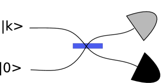
Figure 4: Diagram of a simplified $2$-bin multiplexing detector.

For this simple example, the probability distribution we are after is $p^{2}(j/k)$. We will show how to calculate $p^{2}(j/k)$, $p^{4}(j/k)$ and then how to go from $p^{N}(j/k)$ to $p^{2N}(j/k)$. For the two bin case from Fig. 4 consider a BS with transmittivity $T$ and reflectivity $R$. In that case:

• $p^{2}(j,0)=\delta_{j,0}$ (if no photons are present we will only register zero clicks).

• $p^{2}(1,k)=T^{k}+R^{k}$ (with probability $T^{k}$, $k$ photons end up in the lower bin and the same holds for the upper bin with $R^{k}$. The probability of a single click is the sum of these independent probabilities).

• $p^{2}(2,k)=1-T^{k}+R^{k}$ (if $k\neq 0$ then only two events may happen: one click or two. This complementary event has therefore $P=1-$ (Probability of $1$ click).)

In the case of a $4$-bin detector shown in Fig. 5, $k$ incoming photons are distributed to two $2$-bin detectors according to a binomial distribution.

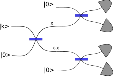
Figure 5: Diagram of a simplified $4$ bin multiplexing detector. The first beam splitter distributes $k$ photons according to a binomial distribution between the two $2$-bin loopies of the second stage.

Now let us evaluate the probability for the upper $2$-bin detector to register $s$ counts if $x$ photons entered while registering $m$ clicks in the lower 2-bin detector if $k-x$ entered the lower port. This should be $p^{2}(s,x)p^{2}(m,k-x)$ weighted by the probability that $x$ photons enter the upper branch and $k-x$ the lower one, which is

$$\binom{k}{x}T^{k-x}R^{x}.$$

Now the probability that $j$ counts are found overall is found summing the weighted probability over all possible ways that the detectors can find $j$ counts (i.e., $m+s=j$) and summing over all possible ways of distributing $k$ photons:

$$p^{4}(j/k)=\sum_{x=0}^{k}\sum_{m+s=j}\binom{k}{x}T^{k-x}R^{x}p^{2}(s,x)p^{2}(m,k-x).$$

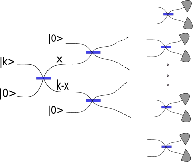
Figure 6: Diagram of a $2N$-bin multiplexing detector. The first beam splitter distributes $k$ photons according to a binomial distribution between the two next $N$-bin stages.

We can extend the same argument to $2N$. Imagine we know $p^{N}(j/k)$. Now, for that detector to become a $2N$-bin detector all we need is to couple two of them to a beam splitter which will distribute the $k$ photons as described above and as shown in Fig. 6. In that same fashion we can then define the recursive relation

$$p^{2N}(j/k)=\sum_{x=0}^{k}\sum_{m+s=j}\binom{k}{x}T^{k-x}R^{x}p^{N}(s,x)p^{N}(m,k-x).$$ (11)

This of course can be generalized to accommodate a different BS reflectivity at each node (adding an index to $T$ and $R$ to account for its position). Based on this recursion and once we determine all $T$ and $R$, we can write a simple and efficient program to generate the corresponding theoretical POVMs. For example, a $6$-outcome detector would have a POVM which can be captured in the following matrix:

$$\begin{array}[c]{lcccccc}&\pi_{0}&\pi_{1}&\pi_{2}&\pi_{3}&\pi_{4}&\pi_{5}\\ |0\rangle\langle 0|&1&0&0&0&0&0\\ \vskip 6.0pt plus 2.0pt minus 2.0pt\cr|1\rangle\langle 1|&0&1&0&0&0&0\\ \vskip 6.0pt plus 2.0pt minus 2.0pt\cr|2\rangle\langle 2|&0&0.128&0.871&0&0&0\\ \vskip 6.0pt plus 2.0pt minus 2.0pt\cr|3\rangle\langle 3|&0&0.0168&0.334&0.648&0&0\\ \vskip 6.0pt plus 2.0pt minus 2.0pt\cr|4\rangle\langle 4|&0&0.00226&0.100&0.495&0.400&0\\ \vskip 6.0pt plus 2.0pt minus 2.0pt\cr|5\rangle\langle 5|&0&0.000309&0.0283&0.265&0.508&0.197\\ \vskip 6.0pt plus 2.0pt minus 2.0pt\cr|6\rangle\langle 6|&0&0.0000428&0.00772&0.123&0.421&0.447\\ \vskip 6.0pt plus 2.0pt minus 2.0pt\cr|7\rangle\langle 7|&0&0.00000601&0.00208&0.0536&0.291&0.653\\ \vskip 6.0pt plus 2.0pt minus 2.0pt\cr|8\rangle\langle 8|&0&0.000000852&0.000565&0.0224&0.181&0.794\end{array}$$

where $B_{k,j}=p^{5}(j/k)$, $\;j=0,\dots,5$ and $k=0,\dots,8$. For example, the $5$-click event has a POVM element,

$$\pi_{5}\simeq 0.2|5\rangle\langle 5|+0.4|6\rangle\langle 6|+0.6|7\rangle\langle 7|+0.8|8\rangle\langle 8|,$$

etc. More generally, the measured statistics are related to the incoming photons by

$$p_{j}=\sum_{k}p^{N}(j/k)\;q_{k},$$

where $p_{j}$ is the probability of detecting $j$ counts and $q_{k}$ the probability that $k$ photons arrived to the TMD loopy0 . The Matrix $\mathbf{B}$ introduced above then relates probabilities and density matrices through: $\mathbf{p}=\mathbf{B}\cdot\mathbf{\rho}$.

IV.2 Detector loss

TMD detectors have various sources of loss, meaning that photons are absorbed before triggering a detection event. The major sources of loss are the coupling to the fibres, the absorption and scattering in the delay fibres and the non-unit efficiency of the detectors achilles-2006-97 . A full description of the effect of losses is certainly complex, since loss occurs at many stages of the detector. One can model loss simply as a beamsplitter diverting photons out of an input state. However, one would have to include a BS before the detector (fibre coupling), a BS at each stage of fibre and a BS in front of each APD, altering Eq. (11) accordingly. Instead we give an effective description modeling loss with a single BS in front of the detector. The matrix capturing the losses has entries that are given by

$$L_{k^{\prime},k}=\binom{k}{k^{\prime}}\eta^{k^{\prime}}(1-\eta)^{k-k^{\prime}},$$

being the binomial distribution accounting for loss since $L_{k^{\prime},k}=0$ for all $k<k^{\prime}$. Now combining both descriptions, we can decouple the loss from the binning, putting a BS coupled to the environment before the $N$-bin TMD resulting in

$$p_{j}=\sum_{k,k^{\prime}}p^{N}(j/k^{\prime})L_{k^{\prime},k}\;q_{k}.$$

This relationship expresses how the incoming photons experience loss and then are distributed among the available modes. The model of the TMD described up to this point would be the one needed without detector tomography. One could for example try to measure independently the transmittivities of the inner BS, reconstruct the convolution (or binning) matrix $\mathbf{B}$ and try to estimate the overall loss to include it in the matrix $L$. This would help us build a model of the TMD sketched in Fig. 7. By contrast, using detector tomography, we do not need to know anything about bins, beam splitters, inner detectors or specific loss mechanisms. Moreover, anything left out of our detector model (e.g. dark counts, afterpulsing, etc.) would be included in a tomographic characterization.

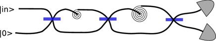
Figure 7: Diagram of a simplified 8 bin time multiplexing detector (TMD). The spirals represent a delay in the optical fibre.

V Experimental reconstruction

We now turn to the description of the experimental realisation. As mentioned earlier, coherent states are ideal probe states with which to characterize optical detectors. This holds true for any optical detector, including polarization detectors, frequency detectors (e.g. spectrometers), and even detectors that discriminate inherently quantum states (e.g. a photonic Bell-state detector). In most of these cases, we are only interested in the detector’s action at a particular input photon number $n$ (usually $n=1$). Still, we can reconstruct the detector POVM in the full photon number basis and then restrict our attention to a particular subspace. It is interesting that an optical state which can be fully described in a classical theory of electromagnetism can be used to characterize uniquely quantum detectors. To characterize a completely unknown detector (i.e. a black box) one would need to vary all the available parameters of the probe set of coherent states: spatial-temporal mode, polarization, phase, and amplitude (ensuring a tomographically complete set of states is constructed). However, given that frequency, time, position, momentum, and amplitude have infinite range, this is impossible in practice. Consequently, one is required to make realistic assumptions about the range of operation and sensitivity of any unknown detector. One might additionally neglect some of these optical parameters if one is only interested in a particular aspect of the full characterization.

The subjects of our detector tomography, the APD and TMD, possess the unique features of single-photon sensitivity and photon-number resolution, respectively. To characterize these features we vary only the amplitude and phase of probe coherent states, while fixing the spatial-temporal mode. In particular, the input wavepackets have a time extent shorter than the time window of the electronics, and the center wavelength is within range of the detectors. Light is coupled to both types of detector through single-mode optical fiber, eliminating the possibility of any variation in the position or momentum mode of the light. Critically, for the detectors to perform as intended and in order to ensure the detectors are memoryless, the wavepackets must be preceded and followed by time intervals in which there is no input light. The APD is known to have a deadtime of roughly $50$ ns; a detection that occurs before the input wavepacket arrives at the detector will make the detector insensitive to the probe coherent state. The TMD splits the incoming wavepacket into time bins spread over $500$ ns. The inverse of these two timescales then sets an upper limit on the rate at which we can send probe states to the detectors. We further limit the rate to ensure the detectors do not heat up, which would change their properties over time. These time variant features of the detectors could be illuminated with detector tomography but this would be unnecessarily complicated, as they are quickly evident without use of the full tomography procedure.

When operated with a gain high above their lasing threshold, lasers produce light well approximated by a coherent state. Coherent states (and statistical mixtures thereof) are unique amongst pure optical states in that, at a beamsplitter, the transmitted and reflected states are unentangled. Consequently, through attenuation we can vary the amplitude of a coherent state without changing its nature. In homodyne state tomography, one must use a balanced detection technique to negate technical noise in the laser. In contrast, by attenuating the laser light to the single-photon level in our detector tomography scheme, the resulting coherent state possesses an inherent amplitude uncertainty that renders the technical noise insignificant.

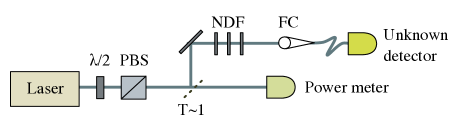
Figure 8: Experimental setup: The amplitude of the probe coherent state is attenuated with a half-waveplate ($\lambda/2$) and a Glan-Thompson polarizer (P). The light is then further attenuated by Frequency independent filters or Neutral Density Filters (NDF) and coupled into a fibre (FC)

We use a cavity dumper (APE Cavity Dumper Kit) to reduce the repetition rate of a pulsed mode-locked Ti:sapph laser to $R$. Long term drift of the laser power over 1 million pulses was $<0.5\%$. Our laser randomly varies in energy between subsequent pulses with a standard deviation of $1.88\%\pm 0.02\%$ of $\left|\alpha\right|^{2}$. We vary the amplitude $\alpha$ of our probe coherent states by rotating their polarization with a half-waveplate ($\lambda/2$) in front of a Glan-Thompson polarizer (P) as shown in Fig. 8. We attenuate the coherent states by reflecting them from a beamsplitter (BS) ($T$=95%) and three neutral density filters (NDF) (i.e. spectrally flat attenuators). Note that $R/T$ for the BS was measured with a relative deviation smaller than $1\%$. Along with some loss upon coupling into a single-mode fiber, we collect these attenuations together in an overall attenuation factor $\gamma$. We test for any variation in $\gamma$ as a function of $\alpha$ (e.g. which might be caused by rotating the waveplate if it had a wedge) and find that the variation is less than $1\%$.

There are, as of yet, no direct techniques to calibrate the power of light at the single-photon level Worsley09 . In fact, there are no laboratory methods to make an absolute calibration of power at any intensity. Instead, a chain of photo-detectors are calibrated relative to each other. At the beginning of the chain is an absolute calibration system held at national standards institutes. In the case of our power meter (Coherent FieldMaxII-TO), the National Institute for Standards and Technology (NIST) uses a cryogenic bolometer as its absolute standard. This chain results in a 5% systematic uncertainty in our measurements of the laser power $P$ (averaged over 0.2s), measured at the transmitted port of the beamsplitter. The magnitude of $\alpha$ for the probe state was found via $\left|\alpha\right|^{2}=$ $\gamma P\lambda/(Rhc)$. For each value of $\alpha$ we recorded the number of times each detection outcome occurred in $J$ trials (i.e. laser pulses), which provides an estimate of $p_{\alpha,n}$. The phase of $\alpha$ was allowed to drift freely, during which no change in the $p_{\alpha,n}$ was observed. Consequently, we did not actively vary the phase of our probe states.

The 5% uncertainty in $P$ is the dominant error in our experiment. For a detector with over 95% efficiency, this error could result in estimates of $\left\{p_{\alpha,n}\right\}$ that are incompatible with any physical detector. For example, this could result in more detector clicks on average than there were photons in the probe state on average. Gain in the detector could achieve this, but at the same time would necessarily introduce noise that would change the distribution of $p_{\alpha,n}$. For detectors with lower efficiency, the systematic error in $P$ will simply add or subtract from efficiency of the detector that results from the tomographic characterization.

We choose a center wavelength $\lambda$ and a FWHM bandwidth of $\Delta\lambda$ that are appropriate for each detector. In the case of the APD detector (a Perkin Elmer SPCM-AQR-13-FC) we set $\lambda=780\pm 1$ nm, $\Delta\lambda=20$ nm, and chose the appropriate rate $R=1.4975\pm 0.0005$ kHz, $J=1472967$, and $\gamma=(5.66\pm 0.08)\times 10^{-9}$. For the TMD detector we set $\lambda=789\pm 1$ nm, $\Delta\lambda=26$ nm, $R=76.169\pm 0.001$ kHz, $J=38084$, and $\gamma=(8.51\pm 0.11)\times 10^{-9}$.

Since $\left|\alpha\right|^{2}$ has an infinite range, one must set an upper limit on the magnitude of $\alpha$ used in our set of probe states. A natural place for this is at the $\alpha$ at which the detector behavior saturates, i.e. $p_{\alpha,n}$ stays constant as a function of $\alpha$. Since this occurs asymptotically, a somewhat arbitrary degree of constancy must be chosen; we set $\left|\alpha\right|^{2}=120$ as our upper limit. We expected the saturation behavior of the TMD would be $p_{\alpha,n}\approx 100\%,$whereas we found that it was $p_{\alpha,8}=93.3\%$ and $p_{\alpha,7}=6.7\%.$ Already, the measured statistics (which are proportional to $Q_{n}(\alpha)$) give a clear signature that our theoretical model of the detector is too simplistic. Moreover, as we increase the $\alpha$ beyond our upper limit $p_{\alpha,8}$ begins to decrease. The cause for this behavior is a break down of our memoryless detector assumption and highlights how crucial it is to create probe states in the desired spatial-temporal mode. Along with the probe laser pulse, the cavity dumper also out-couples a small fraction of the preceding and following pulses in the Ti:Sapph cavity. These are separated in time from our probe pulse by $13$ ns and each contain only $0.17\%$ the energy of the probe pulse. Consequently, these extra pulses will have an insignificant effect on $p_{\alpha,n}$ for most of the range of $\alpha$. However, at $\left|\alpha\right|^{2}=120$, the preceding pulse will be a coherent state with $\left|\alpha\right|^{2}=0.2$. Consequently, roughly $20\%$ of the time bins in the TMD will be preceded by a photon. If the detector has, for instance, a $50\%$ efficiency then $10\%$ of the time bins will be preceded by a detection event that will not be counted as click by the electronics (due to their time window). More importantly, those bins will subsequently be unavailable to detect photons in our probe pulse, due to the $50$ ns deadtime of the APDs inside the TMD. Thus, as we observe, roughly $10\%$ of the bins will not result in a click. This behavior was extraneous to the normal operation of the detector and so we limit $\left|\alpha\right|^{2}$ to $30$ in the tomographic reconstruction. However, it exemplifies the usefulness of even the basic detector tomography procedure, which results in approximate $Q_{n}(\alpha)$, for rough evaluation of the detector action. Some of these hypothesis or details could be further explored if we knew well some detectors or some states. For example the response of BS and neutral density filters to single photons could be explored (granted good single photons and reliable single photon detectors). The time independence of the POVMs could also be studied with well known states. However, we will see that the excellent fit of the data to the Q-function and of the reconstruction to the model suggests a sufficiently good understanding.

V.1 Results

We now turn to the tomographic reconstruction. To characterize our detector we have measured the outcome probability distributions resulting from sending a tomographically complete set of input states (or probe states). The use of pure coherent states as probe states implies that the probability distribution is proportional to the Q-function, as seen in Eq. (3). In principle the knowledge of the Q-function is then sufficient to predict the measurement probabilities for any incoming state since $Q(\alpha,\alpha*)=\langle\alpha|\rho|\alpha\rangle$ determine $\rho$ completely.

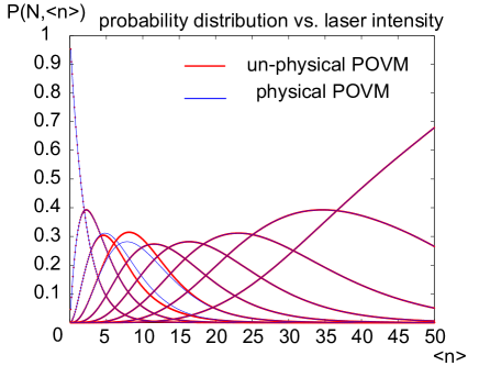
Figure 9: This plot presents the probability distributions corresponding to two detectors. One with negative “POVM” elements and anotherone with positive ones. Both POVMs observe $\sum{\pi_{n}}=\mathbbm{1}$.

However, a more useful and natural representation for photodetectors is the POVM expanded in the Fock basis. Another argument to find the POVM elements is that due to statistical noise, the Q-function could correspond to a non-physical POVM. Indeed, if we simply make a fit to the noisy measured probability distribution, this fit could correspond to negative “POVMs”. As an example consider Fig. 9 where two Q-functions are displayed together: Even though they are very similar to each other, one corresponds to a detector with a non-positive “POVM” element (and thus negative probabilities) and one corresponds to a physical one. Our goal is therefore to reconstruct the POVM operators which most closely match the data and still observe Quantum Mechanics (and thus are positive). .

Since we adopt a “black box” approach we need not assume any of the properties described in the previous theoretical models. Only the accessible parts of the “black box”  i.e., number of outcomes and control (or lack of control) of the phase will determine the description of our detector. The lack of a phase reference simplifies the experimental procedure, allowing us to solely control the magnitude of $\alpha$ (as has been done for tomography of a single photon Lvovsky ). A detector with no observed phase dependence will be described by POVM elements diagonal in the number basis,

$$\pi_{n}=\sum_{k=0}^{\infty}\theta_{k}^{(n)}|k\rangle\langle k|,$$

simplifying hence the reconstruction of $\pi_{n}$.

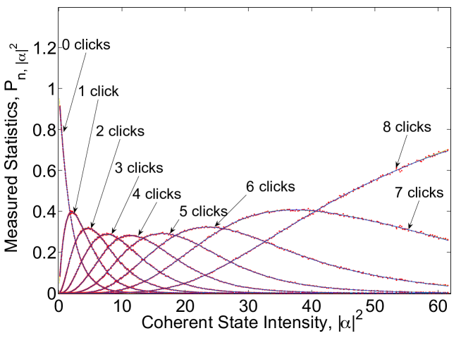
Figure 10: The measured probabilities for different “number-of-clicks” are shown (red dots) as a function of $|\alpha|^{2}=\langle n\rangle$. The plot shows the statistics for the time multiplexed detector (TMD) with $9$ time-bins. The statistical error vertically is too small to be seen and the jitter of $|\alpha|^{2}$ was estimated to be $2$% of its value. An additional $5$% systematic error in the calibration of the power meter is present but can be absorbed as loss. From the reconstructed POVM elements $\left\{\pi_{n}\right\}$ we generate the corresponding probability distributions $\text{tr}(\rho_{\alpha}^{\mathrm{(in)}}\pi_{n})$ (blue curves). These are generated for pure $|\alpha\rangle\langle\alpha|$ or mixed $\rho_{\alpha}^{\mathrm{(in)}}$ and for $\pi_{n}$ reconstructed with the filter function or without it. For all these options, the probability distributions (blue lines) are so similar that they are indistinguishable on this scale.

Again we can express the relationship between the statistics and our diagonal $\pi_{n}$ as,

$${P}=F\Pi,$$

if we measure $D$ different values of $\alpha,\alpha_{1},\dots,\alpha_{D}$, and truncate the number states at a sufficiently large $M$. For an $N$-outcome detector, the matrices will have dimensions $P\in\mathbbm{C}^{D\times N}$, $F\in\mathbbm{C}^{D\times M}$, and $\Pi\in\mathbbm{C}^{M\times N}$. In addition

$$F_{i,k}=\frac{|\alpha_{i}|^{2k}\exp{(-|\alpha_{i}|^{2})}}{k!}$$

can easily be rewritten when the input state is a mixed state. This was done indeed to account for the laser’s technical noise (as we will see in the next section) but gave similar results. For such a detector, the physical POVM consistent with the data can be estimated through the following optimisation problem:

$$\text{min}\left\{\|{P}-F\Pi\|_{2}+g(\Pi)\right\},$$

$$\text{subject to }\;\;\pi_{n}\geq 0,\,\;\;\sum_{n=1}^{N}\pi_{n}=\mathbbm{1},$$ (12)

where the $2$-norm ensures it is a convex quadratic problem. Note that we also allow for convex quadratic filter functions $g$ which will be discussed in some detail later. These $g$ are related to the conditioning of the problem and must not depend on the type of detector. For example, no symmetry or knowledge of the typical POVM structures in photo-detection can be assumed. If any, only general regularization functions that work for any POVM should be chosen. Now, for suitable filter functions (i.e. cuadratic) the whole problem is a convex quadratic optimisation problem, and hence also a semi-definite problem (SDP) which can be efficiently solved numerically Convex . Moreover, in this case, there exists a dual optimisation problem whose solution coincides with the original problem. Thus, the dual problem provides a certificate of optimality since it provides a lower bound to the primal problem.

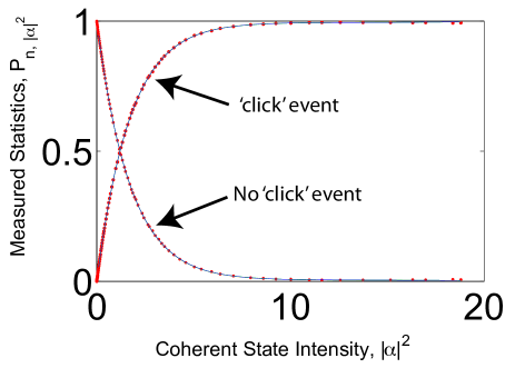
Figure 11: The measured probabilities for the “click” and “no-click” envents in the Avalanche Photodiode (APD) are shown as a function of $|\alpha|^{2}=\langle n\rangle$. The statistical error vertically is too small to be seen and the jitter of $|\alpha|^{2}$ was estimated to be $2$% of its value. An additional $5$% systematic error in the calibration of the power meter is present but can be absorbed as loss. From the reconstructed POVM elements $\left\{\pi_{n}\right\}$ we generate the corresponding probability distributions $\text{tr}(\rho_{\alpha}^{\mathrm{(in)}}\pi_{n})$ (blue curves). These are generated for pure $|\alpha\rangle\langle\alpha|$ or mixed $\rho_{\alpha}^{\mathrm{(in)}}$ and for $\pi_{n}$ reconstructed with the filter function or without it. For all these options, the probability distributions (blue lines) are so similar that they are indistinguishable on this scale.

Care has to be taken that the optimisation problem is well conditioned in order to find the true POVM of the detector. In finding their number basis representation we are deconvolving a coherent state from our statistics which is intrinsically badly conditioned due to the importance of the wings of the Gaussian. Similar issues of conditioning have been discussed in the context of state and process tomography, see, e.g., Refs. UnstableBoulant ; UnstableHradil . Due to a large ratio between the largest and smallest singular values of the matrices defining the quadratic problem, small fluctuations in the probability distribution can result in large variations for the reconstructed POVM. This can result in operators that approximate really well the outcome statistics and yet do not exhibit a smooth distribution in photon-number. We will discuss how to treat this problem in the next section.

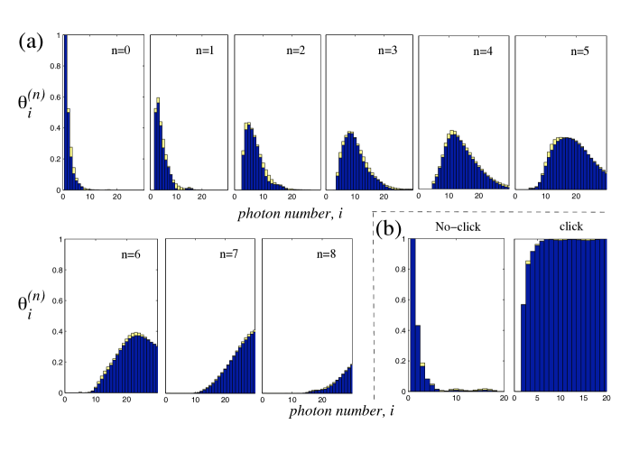
Figure 12: Reconstructed POVMs for (a) the photon-number resolving TMD and (b) the APD “yes/no” detector. TMD POVMs were obtained up to element $|60\rangle\langle 60|$ (therefore $M=60$), but are shown up to $|30\rangle\langle 30|$ for display purposes. APD POVMs are shown in full. Stacked on top of each $\theta_{i}^{(n)}$ where $n$ is the number of clicks we show $|\theta_{i}^{n\mathrm{(\mathrm{rec})}}-\theta_{i}^{n\mathrm{(theo)}}|$ in yellow. “rec” stands for reconstructed and (theo) is the theoretical POVM expected from (a) a TMD modelled with $3$ beam splitters of measured reflectivities and 52.1% overall loss (b) a theoretical APD with $43.2$% loss respectively. Note that this result was obtained with a regularized optimisation as explained in next section .

The measured probabilities for each outcome as a function of $|\alpha|^{2}$ are displayed in Fig. 11 and Fig. 10. The probability distributions (equivalent modulo $1/\pi$ to the Q-function of the detector) show smooth profiles and distinct photon number ranges of sensitivity for increasing number of clicks in the detector. Fig. 12 shows the POVMs that result from the optimisation in Eq. (V.1) which we will discuss later. A first remarkable property is that $\pi_{n},$ being the POVM for $n$ clicks, shows zero amplitude for detecting less than $n$ photons. That is, the detector shows essentially no dark counts. It should be noted that this was not assumed at the outset and is purely the result of the optimization. This sharp feature gives the detector its discriminatory power where $n$ clicks means at least $n$ photons in the input pulse.

To assess the performance of our method we compare it to the model described in the previous section. This time however, the BS used in the model are not 50/50 but its reflectivities ($R=[0.5018,0.5060,0.4192]$) were measured experimentally. This was done measuring the reflected and transmitted beams of a laser with a calibrated power meter. The yellow bars in Fig. 12, show the absolute value of the difference between the theoretical and the reconstructed POVM elements. The magnitude

$$\Delta^{(n,i)}_{\theta}=|\theta_{i}^{(n,\mathrm{theo})}-\theta_{i}^{(n,\mathrm{rec})}|$$

is shown stacked on top of each coefficient of the POVM elements where (theo) stands for theoretical and (rec) for reconstructed. The small yellow bars reveal a good agreement with the model. We also calculate a form of fidelity finding that

$$F=\mathop{\rm Tr}{}\left(\left(({\pi_{n}^{\mathrm{\mathrm{(theo)}}}})^{\frac{1}{2}}\pi_{n}^{\mathrm{\mathrm{(rec)}}}({\pi_{n}^{\mathrm{\mathrm{(theo)}}}})^{\frac{1}{2}}\right)^{\frac{1}{2}}\right)^{2}\geq 98.7\%$$

holds for all $n$. Note that to calculate $F$ we normalized the POVM elements. This overlap indicates an excellent agreement between the two.

In addition, one can reconstruct a probability distribution: from the found POVMs to fit the data. The reconstruction is plotted as dark blue bars in Fig. 10 and Fig. 11. It is the equivalent of the Q-function had our probe states $|\alpha\rangle\langle\alpha|$ with suitable complex $\alpha$ been strictly pure. In fact, although formally distinct, the probability distribution associated with the reconstructed POVM using mixed or pure states are practically indistinguishable and are plotted together in Fig. 10 for comparison.

V.2 Detector Wigner functions

An alternative representation of the detectors which can give us more insight about their structure comes from the quasi-probability distributions such as the Wigner Function UlfBook ; Schleich-book . Since the POVM elements ${\pi_{n}}$ are self adjoint positive-semi-definite operators, a Wigner function $W_{n}$ can be calculated in the standard way from the POVM element $\pi_{n}$:

$$W_{n}(x,p)=\frac{1}{\pi\hbar}\int_{-\infty}^{\infty}dy\,\langle x-y|{\pi}_{n}|x+y\rangle e^{2ipy/\hbar},$$ (13)

where we have, as usual, now identified $(x,p)\in\mathbbm{R}^{2}$ as phase space coordinates of a single mode with $\alpha\in\mathbbm{C}$. However, since the POVMs do not have unit trace, this detector Wigner function will not be normalized,

$$\int_{-\infty}^{\infty}dx\,\int_{-\infty}^{\infty}dp\;W_{n}(x,p)<1.$$ (14)

We should note that the marginals cannot be interpreted as probability distributions but we can still use $W_{n}$ to calculate probabilities according to

$$p_{\rho,n}=\mathop{\rm Tr}{}\left({\rho}{\pi}_{n}\right)=\int_{-\infty}^{\infty}dx\,\int_{-\infty}^{\infty}dp\;W_{\rho}(x,p)W_{n}(x,p).$$ (15)

$\begin{array}[c]{ccc}\includegraphics[width=227.62204pt]{13_Wigner_Overlap_lossy_reconstructed.pdf}&\vline&\includegraphics[width=227.62204pt]{14_small_Wigner_Overlap_perfect_reconstructed.pdf}\\ (a)&&(b)\\ &&\end{array}$

Figure 13: Wigner function of the first POVM elements of the TMD. Since the detectors have no phase reference, their Wigner functions are rotationally symmetric with respect to their center and a cut contains all the information. The dotted blue curve represents the Wigner function of the reconstructed POVMs from $0$ to $5$ clicks. In red we can see the theoretical Wigner function for: (a) a theoretical TMD with 52% loss. (b) a theoretical TMD without loss. Paying attention to the scale we observe how dramatic the effect of loss is at damping the ripples in the Wigner function. It is also worth noting that the end ripples in (a) for the “$5$ click” are just an edge effect due to number state cutoff.

Since none of the detectors have phase sensitivity their Wigner functions are rotationally symmetric around the origin. In Fig. 13 we display a cut of the TMD Wigner function for the following POVM elements:

$$\{\pi_{0},\pi_{1},\pi_{2},\pi_{3},\pi_{4},\pi_{5}\}.$$

Higher clicks are not displayed because their amplitude is too small to be compared with the rest. The interesting feature about the plot is the comparison with the theoretical TMD Wigner functions one can generate with the model. Indeed, comparing a theoretical loss-less TMD with the measured one we see how the amplitude of the Wigner function decreases rapidly for higher photon numbers. On the other hand, comparison with the lossy theoretical model reveals a good agreement.

VI Ill Conditioning and regularisation

One of the main problems encountered in the tomographic characterisation of the detectors has to do with the numerical stability of the reconstruction. Such problems are common in tomography UnstableBoulant ; UnstableHradil . Consider for example the transformations involved in the inverse Radon transform and their inherent instabilities. Note also how going from the Q-function to the P-function is not always well defined Schleich-book . Multiple tools exist to bridge the link between homodyne tomography and the density matrix description lvovsky-pattern . One of them involves the use of pattern functions dariano-pattern ; leonardt-pattern ; wunsche-1997 . That is, finding some functions $G_{k}(\alpha)$ such that

$$\int{\ Q^{(n)}(\alpha)G_{k}(\alpha)d^{2}\alpha}=\theta_{k}^{(n)}.$$

However, finding the appropriate $G_{k}$ involves the irregular wave functions (particular unbounded solutions of the Schrödinger equation) and proving them to be appropriate is typically as hard as estimating the error pattern-fun . The use of maximum likelihood has also been explored and particularly for detector tomography dariano-2004-93 ; PhysRevA.64.024102 . However, the speed of the convergence is not generally guaranteed to be high, becoming exponential for certain problems. Our approach, following the spirit of maximum-likelihood, translates the problem into a quadratic optimisation one allowing for efficient semi-definite programming (SDP) (cf. Eq. (V.1)). We discuss here the details, approximations and filters that lead to our solution of the problem.

VI.1 Truncating the Hilbert space

The data was measured up to $|\alpha|^{2}=150$ but was truncated at lower values in phase space. This was done to avoid noisy behavior and the emergence of new regimes in the behavior of the detector. Memory effects requiring a larger POVM space were thus avoided as discussed in the experimental section. Notably, the effects related to the detector’s dead time, after-pulsing or the dark counts from possible over heating were avoided staying in a low ($|\alpha|^{2}\simeq 70$) photon number regime.

VI.2 Pure vs. mixed

The Q-function of our detector (directly measured) is proportional to

$$p_{\alpha,n}=\mathop{\rm Tr}{}\left(|\alpha\rangle\langle\alpha|\pi_{n}\right).$$ (16)

From Eq. (5) and Eq. (II.4), for a diagonal POVM, we can write the problem as

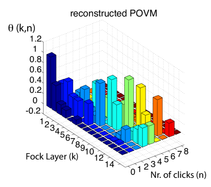
Figure 14: POVM reconstruction, using only minimisation from Eq. (17). Dark blue: $\pi_{0}=\sum_{i=0}^{15}\theta_{i}^{(0)}|i\rangle\langle i|$, lighter blue, $\pi_{1}=\sum_{i=0}^{15}\theta_{i}^{(1)}|i\rangle\langle i|$, etc.

$$\min{\|{P}-F\Pi\|_{2}}.$$ (17)

with the usual constraints $\pi_{n}\geq 0$ and $\sum_{n}\pi_{n}=\mathbbm{1}$. Using a semi-definite solver such as Yalmip, the obtained POVMs $\{\pi_{n}\}$ shows irregular dips and a structure quite dissimilar from what a TMD is expected to do.

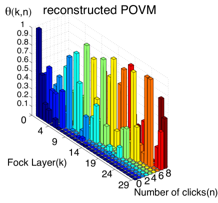
Figure 15: POVM reconstruction, using only minimisation from Eq. (17). Dark blue: $\pi_{0}=\sum_{i=0}^{15}\theta_{i}^{(0)}|i\rangle\langle i|$, lighter blue, $\pi_{1}=\sum_{i=0}^{15}\theta_{i}^{(1)}|i\rangle\langle i|$, etc, displayed up to number layer $30$.

The Fig. 14 shows a typical result, and Fig. 15 shows it for higher photon numbers revealing an even more irregular structure.

VI.2.1 Describing the laser’s amplitude uncertainty

A first meaningful observation is that some level of uncertainty existed in the amplitude $x=|\alpha|^{2}$ of the coherent states. If $D$ values of $x$ were measured then the real

$$\bar{x}=(x_{1},x_{2},,\dots,.,x_{D})$$

might actually have been

$$\bar{x}_{{\delta}}=\left(x_{1}(1+\delta_{1}),x_{2}(1+\delta_{2}),\dots,x_{D}(1+\delta_{D})\right),$$

with some vector of errors $(\delta_{1},\dots,\delta_{D})$. To address the effect of this uncertainty on our minimisation we can artificially introduce noise and then average over many runs of the optimisation. In other words, since $F$ in Eq. (17) depends on the measured values of $|\alpha|^{2}$, we can substitute $\bar{x}$ with $\bar{x}_{{\delta}}$ where $\delta=(\delta_{1},\dots,\delta_{D})$ are independent and identically distributed random variables. Using $\bar{x}_{{\delta}}$ we run the optimisation and obtain a family of estimated POVM elements (each element of the family corresponds to a run of the optimisation with a different $\delta$) As a first approximation we may use a Gaussian probability distribution with zero mean and $\sigma=2\%|\alpha|^{2}$. Note that $2$% was the measured variance of the laser amplitude from pulse to pulse as shown in Fig.  18. Subsequently we average over the POVMs obtained with different “jitters” ${\delta}$ in $N$ realizations, obtaining

$$\pi_{n}^{\mathrm{(average)}}=\sum_{j}{\pi_{n}^{({\delta}_{j})}}/N.$$

$200$ iterations of the optimisation with subsequent averaging improves the appearance of the POVMs but barely solves the “dips” observed. Fig. 16 and Fig. 17 are an example of this approach, showing that this kind of averaging does not properly counteract the fluctuations in the reconstructed POVM.

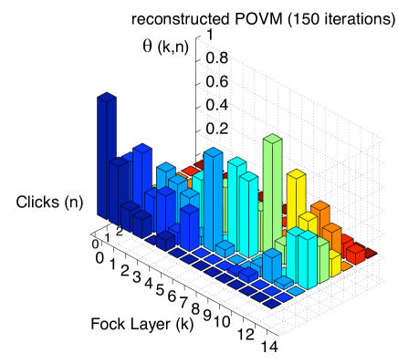
Figure 16: POVM reconstruction, using direct averaging (150 runs with 1% Gaussian noise).

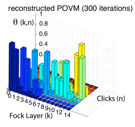
Figure 17: POVM reconstruction, using direct averaging (300 runs with $2$% Gaussian noise).

VI.2.2 Using mixed input states

A key obsevation showing that the previous approach is not the appropriate treatment of uncertainty in $x$ is that each probe state would be best described by a mixture of coherent states,

$$\rho_{x} =\int d^{2}\beta|\beta\rangle\langle\beta|f_{x}(\beta)$$ (18)

$$=\sum_{n,m=0}^{\infty}R_{n,m,x}|n\rangle\langle m|.$$ (19)

Here, $f_{x}$ would be some distribution centered around $x$ in phase space, leading to a mixed Gaussian state in case of a Gaussian classical probability distribution. We can integrate this state $\rho_{x}$ over the complex phase since we have no phase reference available and focus solely on the amplitude of the coherent states or mixtures thereof. Measurements reveal that the intensity of the laser varies from pulse to pulse following a distribution that looks like a Lorentzian with a tail (see Fig.  18).

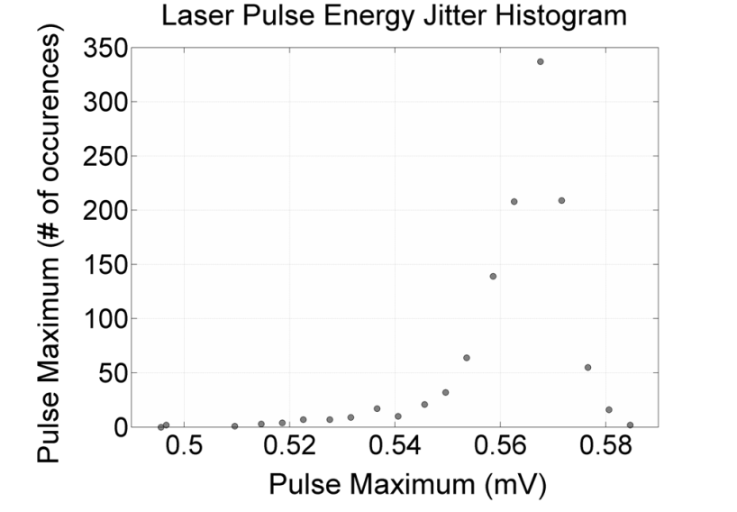
Figure 18: Measurement of the laser’s amplitude variations from pulse to pulse.

A good approximation can however be made using a Gaussian distribution, leading to a Gaussian state, with standard deviation $\sigma=0.02|\alpha|^{2}$, implying

$$R_{n,m,\alpha}=\frac{1}{\sigma\sqrt{2\pi}\sqrt{n!m!}}\int\beta^{n+m}e^{-\beta^{2}}\;f_{x}(\beta)\;d\beta.$$

with $f_{x}(\beta)=e^{-(\beta^{2}-x)^{2}/(2\sigma^{2})}$. The detection probability for outcome $n$ is then

$$p_{n}(\alpha)=\sum_{k=0}^{\infty}R_{k,k,\alpha}\theta_{k}^{(n)}.$$ (20)

To simplify these calculations we can write a distribution in $\sqrt{x}=|\alpha|$,

$$\rho_{|\alpha|}=\int d^{2}\beta|\beta\rangle\langle\beta|\;g_{|\alpha|}(\beta)$$ (21)

with

$$g_{\alpha}(\beta)=e^{-(\beta-\alpha)^{2}/(2\Gamma^{2})}.$$

In this case $\Gamma$ has been chosen such that the approximation $f_{x}(\beta)\simeq g_{\alpha}(\beta)$ holds. These subtleties however do barely alter our results and POVMs are as irregular as previously.

To evaluate the difference introduced by the pure ($|\alpha\rangle\langle\alpha|$) or mixed state ($\rho_{|\alpha|}$) approach we have studied their influence on the reconstructed POVMs. In the regularised optimisation (i.e., for our final results), we have compared the POVMs obtained with each description finding that

$$\frac{\|\Pi_{\mathrm{pure}}-\Pi_{\mathrm{mixed}}\|_{2}}{\|\Pi_{\mathrm{mixed}}\|_{2}}\leq 0.7\%$$ (22)

and the largest relative difference between any two $\theta_{k}^{(n)}$ coming from a mixed state or a pure state derivation was $1.3\%$. Furthermore, the reconstructed probability distributions are so close that they are indistinguishable on the scale of Fig. 10. This reinforces our earlier expectation that technical noise in the laser will be negligible when using single-photon-level coherent states. This differs from homodyne tomography where technical noise can shift a strong local oscillator to a nearly orthogonal state.

However, since the problem of the irregular POVMs is not solved by the mixed state description we need to look further into the origin of these irregularities. One first remarkable (but expected) property is that large variations in the photon number degree of freedom of the POVMs result in minuscule differences in the probability distributions (see Fig. 12). Since one convolutes the photon number distribution with a Gaussian in $\alpha$ to obtain the Q-function this behavior has been expected. Conversely this means that small errors or statistical fluctuations in the Q-function can result in large errors in the POVM elements. Consider for example that if instead of

$$\min{\|{P}-F\Pi\|_{2}}$$

we try to minimise

$$\min{\|F^{-1}{P}-\Pi\|_{2}}$$

the SDP solver finds no sensible solution. This is because using the Moore-Penrose pseudo-inverse we find $F^{-1}F\neq\mathbbm{1}$ due to its inherent ill conditioning, meaning that the ratio of largest and smallest singular values in $F$ is large.

Various methods exist to try and regularise these problems. Whatever the chosen method it should assume as little knowledge as possible about the specific form of the sought POVM. Since $F$ has very small values for high photon numbers one could enhance those values while preserving the minimisation target. For example we could run the optimisation

$$\min{\|{P}D-F\Pi D\|_{2}}$$

where $D$ is a diagonal matrix aimed at regularising the problem. This can be shown to introduce some improvement but does not solve the “dip problem” completely. It is also hard to find the exact form of $D$ that yields “good” results without any prior knowledge about the expected POVMs. In addition (roughly speaking) it is hard to find a balance between having good results for low photon numbers and for high photon numbers.

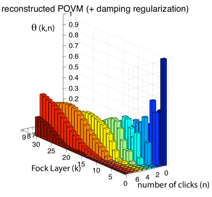
Figure 19: Minimisation using damping method on Eq. (23). Note that the point of view is opposite that of the previous plots. We see some dips around the $5$-th and $7$-th number layer.

Another approach is to introduce a sort of damping or specific penalisation. For example one could define a diagonal matrix $M$ such that

$$M_{i,j}=\delta_{i,j}/j,$$

and use it to redistribute the weight of each POVM element, avoiding unreasonably large POVM element amplitudes (that compensate for low values in $F$). The optimisation could be recast as,

$$\min{\{\|{P}-F\Pi\|_{2}+0.03\|M\Pi\|_{2}\}}.$$ (23)

A result of this can be seen on Fig. 19. This method has the same shortcomings as the previous one: it is sensitive to the choice of parameters and the exact form of $M$ is hard to determine without detailed prior assumptions.

A more reasonable method is to capture the relative smoothness of the POVM from a lossy detector. This method is also called smoothing regularisation Convex . In this case one single assumption needs to be made. The POVMs should exhibit a certain degree of “smoothness”.

VI.3 Smooth or not?

Let us first define what we mean by smooth. Smooth will mean in this context that the difference $|\theta_{k}^{(n)}-\theta_{k+1}^{(n)}|$ is small for all $k$ and $n$. In the optimisation context we will mean that our minimisation is defined as follows:

$$\min{\{\|{P}-F\Pi\|_{2}+y{S}\}}$$ (24)

with

$${S}=\sum_{k,n}(\theta_{k}^{(n)}-\theta_{k+1}^{(n)})^{2}$$

for some fixed value of y. The smoothing function $S$ will be independent of the detector, and will mildly penalize non-smooth POVM elements. This approach is further substantiated by the observation that the resulting POVMs are largely independent of the weight $y$ that is given to the smoothness penalty.

As most quantum detectors, especially those disucussed here are lossy, this is a particularly plausible feature. Indeed, if an optical detector has a POVM element with non-zero amplitude in $|n\rangle\langle n|$, then if it is lossy, it will have a positive amplitude in $|n+1\rangle\langle n+1|$, $|n+2\rangle\langle n+2|,\dots,|n+K\rangle\langle n+K|$, decreasing with $K$ but different from zero. In fact, in general, if the detector has a finite efficiency $\eta$ which can be modelled with a BS, it will impose some smoothness on the distribution $\theta_{k}^{(n)}$. That is because if $G(k)$ is the probability of registering $k$ photons and $H(k^{\prime})$ is the probability that $k^{\prime}$ were present, then the loss process will impose kenny-thesis :

$$G(k)={\displaystyle\sum\limits_{k^{\prime}}}\binom{k^{\prime}}{k}\eta^{k}(1-\eta)^{k^{\prime}-k}H(k).$$

Consequently, if $\theta_{k}\neq 0$, then $\theta_{k+1}$, $\theta_{k+2}$ etc. cannot be zero, but will have some relatively smooth distribution. This simple physical argument makes a certain smoothness plausible (but still should allow sharp transitions for $m<n$).

For this detector (and for any photodiode based detector) assuming loss is reasonable and can make the “smoothness” requirement appropriate. Let us however see if, without looking at the specific shape of our POVM, we can find an optimal smoothing coefficient $y$ and justify further the use of the smoothing regularisation.

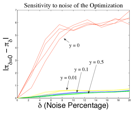
Figure 20: Illustration of the sensitivity to noise for two different minimisation methods ($y=0$ corresponds to no regularisation, and $y\neq 0$ to an approach using a smoothing regularisation). For each value of $y$ and $\delta$ we have run the optimisation $4$ times and displayed the results here to illustrate this variation.

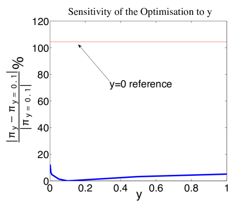
Figure 21: Illustration of how sensitive the optimisation is to the specific choice of $y$. This plot shows the relative error with respect to the POVM elements obtained using $y=0.1$, as a function of $y$. In red, and only for reference (since it does not change with $y$), the value of the relative error for $y=0$ (no smoothing) is shown. We vary $y$ in the range $[0.001,1]$. It is remarkable that a $10000$% variation in $y$ results in only a $12$% variation. For $y\in[0.05,0.2]$ the relative error is less than $2$% in $\Pi$.

One way to test this method is to quantify how resilient it is to noise in the data. To do so we introduce additional noise in $x=|\alpha|^{2}$ to the measured data. For example, we can alter $x$ in ${P}_{i,n}=P(x_{i}(1+\delta_{i}),n)$ where $\delta=(\delta_{1},\dots,\delta_{D})$ is again a vector of random variables distributed with a Gaussian distribution with zero mean. This simulates a statistical uncertainty in the measurement of the coherent state. To see its effect on the reconstruction we use the figure of merit $\|\Pi_{\delta}-\Pi_{\delta=0}\|_{2}$. This quantity should evaluate how POVMs differ from the one without noise. It is seen that the additional smoothing penalty makes the optimisation more robust, largely independent of the value of $y$ (we can multiply $y$ by a $100$ and stay in the same regime). Using this smoothing regularisation with noisy data seems therefore a good choice.

We have seen how smoothing makes the optimization more robust against noise but we should also ask how sensitive this optimisation is to the exact choice of $y$. To do so we may use the following procedure: compare the POVM obtained using $y=0.1$ with that obtained varying $y$ over $4$ orders of magnitude. In Fig. 21 we plot the relative error $\displaystyle{\ 100\ast{|\Pi_{y}-\Pi_{y=0.1}|}/{|\Pi_{y=0.1}|}}$. Remarkably doubling the value of $y$ results in an overall relative error in the POVM of less than $1$%. Multiplying (or dividing) $y$ by 10 gives a variation below $5$% and $100$-fold variation results in a $12$% variation. If we compare how this differs from the $y=0$ case which is $110$% different then we can conclude that the optimisation is quite insensitive to the exact choice of the smoothing parameter $y$. The following table provides some values for reference.

$y$	$y$ variation	$\Pi$ relative error
0.0001	x/1000	27.3%
0.001	x/100	12.2%
0.01	x/10	4%
0.05	x/2	1%
0.5	x 5	3%
1	x 10	5%

Table 1: This table illustrates how sensitive the optimisation is to the particular choice of $y$ (the reference smoothing strenght is $y=0.1$)

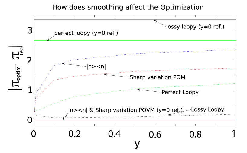
Figure 22: Illustration of how too much smoothing can fail to capture the sharp variations of a POVM. We define $\Pi_{\mathrm{theo}}$ as the matrix containing the POVM elements of the theoretical POVMs. From them we generate a probability distribution and reconstruct the POVMs $\Pi_{\mathrm{optim}}$ with the smoothing regularised optimisation. The dotted lines represent $\|\Pi_{\mathrm{optim}}-\Pi_{\mathrm{theo}}\|_{2}$ for different values of $y$ and for a variety of POVMs (see following plots). The horizontal lines represent that same difference for $y=0$ and are plotted for reference.

VI.4 Sharp and smooth

There is of course a limit to how much we can penalize non-smooth POVMs. Is it possible for the smoothing regularisation to wash out all the sharp features of the POVM, thus smoothing in excess? This of course is a legitimate question that further restricts the reasonable range for $y$. To study that effect we analyse four cases:

1. A theoretical loss-less TMD, based on the model described in Eq. (11).

2. A lossy TMD, based on the above with added loss from an $R=52\%$ BS.

3. A perfect photon number detector, that is with $\pi_{n}=|n\rangle\langle n|$.

4. An artificial POVM with sharp variations, containing the POVM elements:

   $$\pi_{0} = |0\rangle\langle 0|+|2\rangle\langle 2|$$

   $$\pi_{1} = |1\rangle\langle 1|+1/2|3\rangle\langle 3|$$

   $$\pi_{2} = 1/2|3\rangle\langle 3|+|4\rangle\langle 4|+|5\rangle\langle 5|$$

   $$\pi_{3} = |7\rangle\langle 7|$$

   $$\pi_{4} = 1/4|6\rangle\langle 6|+1/4|8\rangle\langle 8|$$

   $$\pi_{5} = 1/4|6\rangle\langle 6|+1/4|8\rangle\langle 8|$$

   $$\pi_{6} = 1/2|6\rangle\langle 6|$$

   $$\pi_{7} = 1/2|7\rangle\langle 7|$$

   $$\pi_{8} = 1/2|8\rangle\langle 8|+\sum_{k=9}^{60}|k\rangle\langle k|$$

   and observing

   $$\sum_{i}\pi_{i}=\mathbbm{1}.$$

To study the smoothing we generate the POVM elements $\{\pi_{n}\}$ numerically, build a probability distribution $\mathop{\rm Tr}{}\left(\rho_{\alpha}\pi_{n}\right)$ and retrieve the $\pi_{n}$ using the optimisation from Eq. (24) for an increasing range of $y$. Then we compare these results with the theoretical POVMs we defined in order to generate the PD. All optimisations are done using the mixed-state approach from Eq. (21). Broadly speaking, we find two distinct behaviors: POVMs with terms that decay slowly in photon number need regularisation and are quite insensitive to the precise $y$. For sharp POVMs (without loss) the range $0<y<0.01$ preserves their shape quite well, but further smoothing hides their true shape. These properties are further illustrated in the figures that follow.

VI.4.1 Lossy TMD

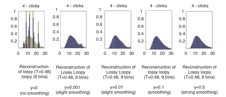
Figure 23: Smoothing evolution for a lossy TMD detector (loss=52%). We show as an example the evolution of the POVM element $\pi_{4}=\sum_{i=0}^{60}\theta_{i}^{(4,{\rm rec})}|i\rangle\langle i|$ as we increase the amount of smoothing (in $y$). The yellow bars display $|\theta_{i}^{(4,{\rm theo})}-\theta_{i}^{(4,{\rm rec})}|$ stacked on top of $\theta_{i}^{(4,{\rm rec})}$ .

Fig. 23 presents the evolution of the “$4$ click” POVM element as we add more smoothing (or increase $y$ in Eq. (24)). This element is chosen as an illustrative example but more details can be found in Ref. Alvaro-Thesis . The figure shows in blue the coefficients $\theta_{i}^{(4)}$ in $\pi^{\mathrm{\mathrm{(rec)}}}_{4}=\sum_{i=0}^{60}\theta_{i}^{(4)}|i\rangle\langle i|$, where (rec) means reconstructed. In yellow, stacked on top of $\theta_{i}^{(4)}$ we display $|\theta_{i}^{(4,\mathrm{rec})}-\theta_{i}^{(4,\mathrm{theo})}|$, where theo refers to the original POVM we used to generate the probability distribution. Clearly the smoothing improves the result and the exact value of $y$ is rather unimportant. A sharp feature that is preserved however is $\theta_{i}^{(4)}=0$ for $i<4$ proving a good agreement with the model.

VI.4.2 Loss-less TMD

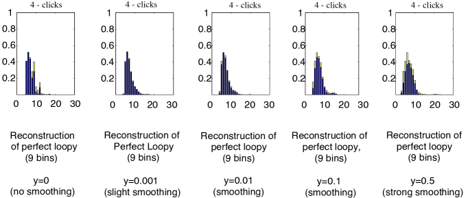
Figure 24: Smoothing evolution for a perfect TMD detector (no loss). We show as an example the evolution of the POVM element $\pi_{4}=\sum_{i=0}^{60}\theta_{i}^{(4,\mathrm{rec})}|i\rangle\langle i|$ as we increase the amount of smoothing (in $y$). The yellow bars display $|\theta_{i}^{(4,\mathrm{theo})}-\theta_{i}^{(4,\mathrm{rec})}|$ stacked on top of $\theta_{i}^{(4,\mathrm{rec})}$.

Fig. 24 shows also the “4 click” event and the error associated with the reconstruction (yellow). This TMD shows in its distribution the finite number of bins as we described earlier. The distribution is not as broad as that of the lossy-loopy and the smoothing is therefore not so effective. The raw SDP, with $y=0$, performs quite well, and the POVM is quite insensitive to the smoothing, although, when given $1/2$ of the weight in the optimisation ($y=0.05$) the smoothing starts to become harmful.

VI.4.3 Perfect number detector

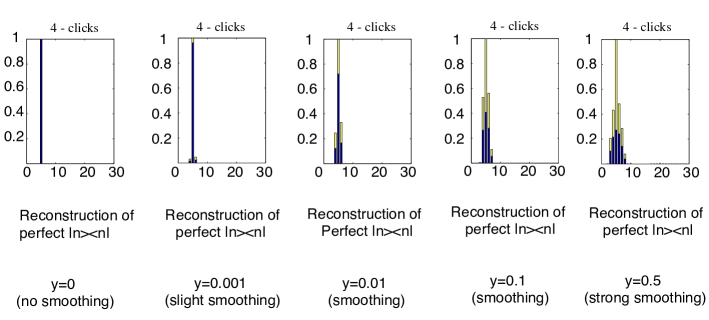
Figure 25: Smoothing evolution for a perfect photon number detector, that is one with $\pi_{n}=|n\rangle\langle n|$. We show as an example the evolution of the POVM element $\pi_{4}=\sum_{i=0}^{60}\theta_{i}^{(4,\mathrm{rec})}|i\rangle\langle i|$ as we increase the amount of smoothing (in $y$). The yellow bars display $|\theta_{i}^{(4,\mathrm{theo})}-\theta_{i}^{(4,\mathrm{rec})}|$ stacked on top of $\theta_{i}^{(4,\mathrm{rec})}$.

Fig. 25 shows also the “$4$ click” event which in this case is simply $\pi_{4}=|4\rangle\langle 4|$. A very interesting feature is that the simple SDP with $y=0$ achieves a perfect result. This happens in spite of using a mixed state as a probe state (mixture of amplitudes $|\alpha|$ around $|\alpha\rangle\langle\alpha|$). The reconstruction is then robust for very well defined and sharp features, where the higher decaying coefficients do not introduce instabilities.

VI.4.4 Sharp POVM

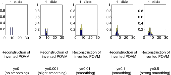
Figure 26: Smoothing evolution for an invented POVM with sharp variations. Displayed is $\pi_{4}=|7\rangle\langle 7|+|9\rangle\langle 9|$. We show as an example the evolution of the POVM element $\pi_{4}=\sum_{i=0}^{60}\theta_{i}^{(4,\mathrm{rec})}|i\rangle\langle i|$ as we increase the amount of smoothing (in $y$). The yellow bars display $|\theta_{i}^{(4,\mathrm{theo})}-\theta_{i}^{(4,\mathrm{rec})}|$ stacked on top of $\theta_{i}^{(4,\mathrm{rec})}$.

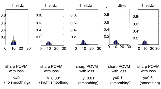
Figure 27: Smoothing evolution for an invented POVM with sharp variations which has suffered a $20$% loss (modelled by interposing a beam splitter).. Displayed is the reconstruction of the element $\pi_{4}=|7\rangle\langle 7|+|9\rangle\langle 9|$ when it suffers the mentionned loss. The reconstruction shows $\pi_{4}=\sum_{i=0}^{60}\theta_{i}^{(4,\mathrm{rec})}|i\rangle\langle i|$ as we increase the amount of smoothing (in $y$). The yellow bars display $|\theta_{i}^{(4,\mathrm{theo})}-\theta_{i}^{(4,\mathrm{rec})}|$ stacked on top of $\theta_{i}^{(4,\mathrm{rec})}$.

We now discuss the situation of a POVM element that is not related to an experiment, but has been artificially generated to identify the limit of the smoothing regularisation. The element displayed in Fig. 26 is $\pi_{4}=|7\rangle\langle 7|+|9\rangle\langle 9|$ and we can see that $y=0.1$ is already too much smoothing. Certainly to reconstruct a completely loss-less detector with such a structure smoothing is not an appropriate strategy. We must remember however that all current photon-number detectors that count particles do exhibit loss, and have therefore some degree of smoothness in them.

VI.4.5 Sharp POVM with loss

The previous case could have given the impression that the reconstruction fails for a sharp POVM. However one has to stress that smoothing (or a regularization for the optimisation) is necessary when there is loss and an ill conditionned matrix (which is a generic case in quantum optics using coherent states for detector tomography). Therefore, it’s worth considering what happens when an invented POVM (as the previous one) is made more realistic adding some loss. Fig. 27 illustrates this, showing the reconstruction of the previous sharp POVM element which has suffered a $20\%$ loss. Indeed in this case we can see a clear improvement as the smoothing helps regularize the optimisation.

VII Conclusion

As quantum information and computation implementations evolve, detectors are becoming more complex. In addition, crypto security requires a careful statement of assumptions idealy kept to a minimum. This, as we have seen, calls for a black-box characterisation of the operators they implement. We have seen the first implementation of this type of tomography. We discussed in detail the first experimental realisation of quantum detector tomography completing the triad of experimental state PhysRevA.40.2847 ; PhysRevLett.70.1244 ; PhysRevA.60.674 , process chuang-1996 ; PhysRevLett.78.390 ; PhysRevLett.80.5465 ; kwiat , and detector tomography NaturePhysTomo . This detector characterisation opens up more flexible and complex ways of detecting quantum states and accurately preparing non-classical light.

The reconstruction methods are simple and efficient. However one has to pay close attention to the subtleties behind the ill-conditioning of such reconstructions whether its state or detector tomography. Fully characterising a detector with this method can help get rid of complex or erroneous assumptions in the modelling. Furthermore, once they are fully characterised, one can re-design or alter the detectors with a direct feedback on their performance.

Detector tomography significantly benefits state tomography or metrology, as well as state preparation and the implementation of protocols in quantum information requiring detectors in state manipulation. Importantly, it enables the use of detectors that are noisy, non-linear or that operate outside their intended range. One conclusion is that lossy detectors are often just as useful as perfect ones, as long as we know the exact POVMs and one can describe the rest of our experiment accordingly. This method will also allow the benchmarking of similar detectors making performance comparisons possible. Indeed one can also ask question concerning the power each detector has for preparing non-classical states. This opens a path for the experimental study of novel concepts such as the non-classicality of detectors. Another promising avenue is to translate homodyne tomography techniques to optical detector tomography. For example defining the detector tomography equivalents of balanced noise-reduction, direct measurement of the Wigner function or pattern functions). Naturally an immediate next step would involve characterizing detectors with off diagonal terms and phase sensitivity.

Acknowledgements

This work has been supported by the EU (COMPAS, HIP, MINOS, Marie Curie, and QAP), the EPSRC, The Heinz-Durr Stipendienprogram of the SDV, the QIP-IRC, Microsoft Research, the EURYI Award Scheme and the Royal Society.

References

- (1) B. L. Higgins, D. W. Berry, S. D. Bartlett, H. M. Wiseman, and G. J. Pryde, Nature 450, 393 (2007).
- (2) K. L. Pregnell, K.J. Resch, R. Prevedel, A. Gilchrist, G. J.Pryde, J. L. O’Brien, and A. G. White, Phys. Rev. Lett. 98, 223601 (2007).
- (3) D. T. Smithey, M. Beck, M. G. Raymer, and A. Faridani, Phys. Rev. Lett. 70, 1244 (1993).
- (4) J. F. Poyatos, J. I. Cirac, and P. Zoller, Phys. Rev. Lett. 78, 390 (1997).
- (5) J. B. Altepeter, D. Branning, E. Jeffrey, T. C. Wei, P. G. Kwiat, R. T. Thew, J. L. O’Brien, M. A. Nielsen, and A. G. White, Phys. Rev. Lett. 90, 193601 (2003).
- (6) R. Raussendorf and H. Briegel, Quant. Inf. Comp. 6, 433 (2002).
- (7) R. Raussendorf, D. E. Browne, and H. J. Briegel, Phys. Rev. A 68, 022312 (2003).
- (8) K. Vogel and H. Risken, Phys. Rev. A 40 (1989).
- (9) K. Banaszek, C. Radzewicz, K. Wódkiewicz, and J. S. Krasiński, Phys. Rev. A 60, 674 (1999).
- (10) I. L. Chuang and M. A. Nielsen, quant-ph/9610001 (1996).
- (11) G. M. D’Ariano and L. Maccone, Phys. Rev. Lett. 80, 5465 (1998).
- (12) M. Lobino, D. Korystov, C. Kupchak, E. Figueroa, B. C. Sanders, and A. I. Lvovsky, Science 322, 563 (2008).
- (13) A. Luis and L. L. Sánchez-Soto, Phys. Rev. Lett. 83, 3573 (1999).
- (14) G. M. D’Ariano, L. Maccone, and P. L. Presti, Phys. Rev. Lett. 93, 250407 (2004).
- (15) J. Fiurášek, Phys. Rev. A 64, 024102 (2001).
- (16) H. B. Coldenstrodt-Ronge, J. S. Lundeen, K. L. Pregnell, A. Feito, B. J. Smith, W. Mauerer, C. Silberhorn, J. Eisert, M. B. Plenio, and I. A. Walmsley, J. Mod. Opt. 56, 432 (2008).
- (17) J. S. Lundeen, A. Feito, H. Coldenstrodt-Ronge, K. L. Pregnell, Ch. Silberhorn, T. C. Ralph, J. Eisert, M. B. Plenio, and I. A. Walmsley, Nature Physics 5, 27 (2009).
- (18) S. Boyd and L. Vandenberghe, Convex optimization (Cambridge University Press, 2004).
- (19) V. Makarov, A. Vadim, A. Anisimov, and J. Skaar, Phys. Rev. A 74, 022313 (2006).
- (20) Ll. Masanes, Phys. Rev. Lett. 102, 140501 (2009).
- (21) Ll. Masanes, R. Renner, A. Winter, J. Barrett, and M. Christandl, quant-ph/0606049.
- (22) W. van Dam, F. Magniez, M. Mosca, and M. Santha, SIAM Journal on Computing, 37(2), 611 (2007).
- (23) M. Freitag, Y. Martin, J.A. Misewich, R. Martel, and Ph. Avouris, Nano Lett. 3, 1067 (2003).
- (24) M. Sasaki, K. Wakui, J. Mizuno, M. Fujiwara, and M. Akiba, AIP Conf. Proc., Quantum Communication, Measurement and Computing, 734, 44 (2004).
- (25) J. Kim, S. Takeuchi, Y. Yamamoto, and H. H. Hogue, App. Phys. Lett. 74, 902 (1999).
- (26) A. J. Shields, M. P. O’Sullivan, I. Farrer, D. A. Ritchie, R. A. Hogg, M. L. Leadbeater, C. E. Norman, and M. Pepper, App. Phys. Lett. 76, 3673 (2000).
- (27) G. N. Gol’tsman, O. Okunev, G. Chulkova, A. Lipatov, A. Semenov, K. Smirnov, B. Voronov, A. Dzardanov, C. Williams, and R. Sobolewski, App. Phys. Lett. 79, 705 (2001).
- (28) A. J. Miller, S. Woo Nam, J. M. Martinis, and A. V. Sergienko, App. Phys. Lett. 83, 791 (2003).
- (29) D. Achilles, C. Silberhorn, C. Sliwa, K. Banaszek, and I. A. Walmsley, Opt. Lett. 28, 2387 (2003).
- (30) D. Achilles, C. Silberhorn, C. Sliwa, K. Banaszek, I. A. Walmsley, M. J. Fitch, B. C. Jacobs, T. B. Pittman, and J. D. Franson, J. Mod. Opt. 51, 1499 (2004).
- (31) D. E. Browne, J. Eisert, S. Scheel, and M. B. Plenio, Phys. Rev. A 67, 062320 (2003).
- (32) J. Eisert, D. E. Browne, S. Scheel, M. B. Plenio, Ann. Phys. (NY) 311, 431 (2004).
- (33) J. Eisert, M. B. Plenio, D. E. Browne, S. Scheel, and A. Feito, Optics and Spectroscopy 103, 181 (2007).
- (34) A. Ourjoumtsev, A. Dantan, R. Tualle-Brouri, P. Grangier, Phys. Rev. Lett. 98, 030502 (2007).
- (35) S. Olivares, M. G. A. Paris, and R. Bonifacio, Phys. Rev. A 67, 032314 (2003).
- (36) T. Opatrny, G. Kurizki, and D.-G. Welsch, Phys. Rev. A 61 032302 (2000).
- (37) R. Garcia-Patron Sanchez, J. Fiurasek, N. J. Cerf, J. Wenger, R. Tualle-Brouri, and Ph. Grangier, Phys. Rev. Lett. 93, 130409 (2004).
- (38) G. Adesso, F. Dell’Anno, S. De Siena, F. Illuminati, and L. A. M. Souza, Phys. Rev. A 79, 040305(R) (2009).
- (39) I. Prochazka, A. L. Migdall, A. Pauchard, et. al, Proc. SPIE 6583, 658302 (2007).
- (40) G. Brida, I. P. Degiovanni, V. Schettini, S. V. Polyakov, A. Migdall, J. Mod. Opt. 56, 405 (2009).
- (41) Y. H. Kim and W. P. Grice, Phys. Rev. A 68, 062305 (2003).
- (42) A. B. U’ren, E. Mukamel, K. Banaszek and I. A. Walmsley, Phil. Trans. R. Soc. Lond. A 361, 1493 (2003).
- (43) N. Boulant, T. F. Havel, M. A. Pravia, and D. G. Cory, Phys. Rev. A 67, 042322 (2003).
- (44) D. N. Klyshko, Sov. J. Quantum Electron. 10, 1112 (1980).
- (45) J. D. Rarity, K. D. Ridley, and P. R. Tapster, Applied Optics 26, 4616 (1987).
- (46) A. Czitrovszky, A. Sergienko, P. Jani, and A. Nagy, Metrologia 37, 617 (2000).
- (47) K. M. R. Audenaert and M. B. Plenio, New J. Phys. 8, 266 (2006).
- (48) J. Eisert, F. G. S. L. Brandão, and K.M.R. Audenaert, New J. Phys. 9, 46 (2007).
- (49) O. Guehne, M. Reimpell, and R. F. Werner, Phys. Rev. Lett. 98, 110502 (2007).
- (50) O. Guehne and G. Toth, Phys. Rep. 474, 1 (2009).
- (51) H. Wunderlich, M. B. Plenio, arXiv:0902.2093.
- (52) U. Leonhardt, Rep. Prog. Phys. 66, 1207 (2003).
- (53) H. B. Coldenstrodt-Ronge and C. Silberhorn, J. Phys. B 40, 3909 (2007).
- (54) M. B. Plenio, unpublished (2007).
- (55) D. Achilles, C. Silberhorn, C. Sliwa et al., J. Mod. Opt. 51, 1499 (2004)
- (56) D. Achilles, C. Silberhorn, and I. A. Walmsley, Phys. Rev. Lett. 97, 043602 (2006).
- (57) A. P. Worsley et al., Optics Express 17, 4397 (2009).
- (58) G. M. D’Ariano, U. Leonhardt, and H. Paul, Phys. Rev. A 52, R1801 (1995).
- (59) A. Feito, Tools and methods for the distillation of entanglement in continuous variable quantum optics, PhD thesis (Imperial College London, 2008).
- (60) M. Ježek, J. Fiurášek, and Z. Hradil, Phys. Rev. A 68, 012305 (2003).
- (61) W. P. Schleich, Quantum optics in phase space (Wiley-VCH, Berlin, 2001).
- (62) U. Leonhardt, Measuring the quantum state of light (Cambridge University Press, 1997).
- (63) U. Leonhardt, M. Munroe, T. Kiss, T. Richter, and M. G. Raymer, Opt. Commun. 127, 144 (1996).
- (64) U. Leonhardt, H. Paul, and G. M. D’Ariano, Phys. Rev. A 52, 4899 (1995).
- (65) A. I. Lvovsky, H. Hansen, T. Aichele, O. Benson, J. Mlynek, and S. Schiller, Phys. Rev. Lett. 87, 050402 (2001).
- (66) A. I. Lvovsky and M. G. Raymer, quant-ph/0511044.
- (67) K. L. Pregnell, Retrodictive quantum state engineering, PhD thesis (Center for Quantum Computer Technology, Griffith University, 2005).
- (68) A. Wünsche, J. Mod. Opt. 44 2293 (1997).