$Q$-system Cluster Algebras, Paths and Total Positivity

$\boldsymbol{Q}$-system Cluster Algebras, Paths
and Total Positivity

Philippe DI FRANCESCO ^† and Rinat KEDEM ^‡

P. Di Francesco and R. Kedem

^† Institut de Physique Théorique du Commissariat à l’Energie Atomique, Unité de Recherche
^† associée du CNRS, CEA Saclay/IPhT/Bat 774, F-91191 Gif sur Yvette Cedex, France

philippe.di-francesco@cea.fr http://ipht.cea.fr/en/Phocea/Pisp/visu.php?id=14

^‡ Department of Mathematics, University of Illinois Urbana, IL 61801, USA rinat@illinois.edu http://www.math.uiuc.edu/~rinat/

Received October 15, 2009, in final form January 15, 2010; Published online February 02, 2010

In the first part of this paper, we provide a concise review of our method of solution of the $A_{r}$ $Q$-systems in terms of the partition function of paths on a weighted graph. In the second part, we show that it is possible to modify the graphs and transfer matrices so as to provide an explicit connection to the theory of planar networks introduced in the context of totally positive matrices by Fomin and Zelevinsky. As an illustration of the further generality of our method, we apply it to give a simple solution for the rank 2 affine cluster algebras studied by Caldero and Zelevinsky.

cluster algebras; total positivity

05E10; 13F16; 82B20

1 Introduction

Discrete dynamical systems may take the form of recursion relations over a discrete time variable, describing the evolution of relevant physical quantities. Within this framework, of particular interest are the discrete integrable recursive systems, for which there exist sufficiently many conservation laws or integrals of motion, so that their solutions can be expressed in terms of some initial data. Interesting examples of such systems of non-linear integrable recursion relations arise from matrix models used to generate random surfaces, in the form of discrete Toda-type equations [2, 18, 23]. More recently, a combinatorial study of intrinsic geometry in random surfaces has also yielded a variety of integrable recursion relations, also related to discrete spatial branching processes [5].

We claim that other fundamental examples are provided by the so-called $Q$-systems for Lie groups, introduced by Kirillov and Reshetikhin [21] as combinatorial tools for addressing the question of completeness of the Bethe ansatz states in the diagonalization of the Heisenberg spin chain based on an arbitrary Lie algebra. We proved integrability for these systems in the case of $A_{r}$ in [8]. In the case of other Dynkin diagrams, evidence suggests integrability still holds.

The $Q$-system with special (singular) initial conditions was originally introduced [21] as the recursion relation satisfied by the characters of special finite-dimensional modules of the Yangian $Y({\mathfrak{g}})$, the so-called Kirillov–Reshetikhin modules. Remarkably, in the case ${\mathfrak{g}}=A_{r}$, the same recursion relation also appears in other contexts, such as Toda flows in Poisson geometry [16], preprojective algebras [15] and canonical bases [4].

In [8], we used methods from statistical mechanics to study the solutions of the $Q$-system associated with the Lie algebra $A_{r}$, for fixed but arbitrary initial conditions. Our approach starts with the explicit construction of the conserved quantities of the system, which appear as coefficients in a linear recursion relation satisfied by $Q$-system solutions. These are finally used to reformulate the solutions in terms of partition functions for weighted paths on graphs, the weights being entirely expressed in terms of the initial data.

Note that there is a choice of various sets of $2r$ variables which constitute an initial condition fixing the solutions of the $Q$-system recursion relation, a choice parametrized by Motzkin paths of length $r$. This set of initial variables determines the graphs and weights which solve the problem. This is the key point addressed in [8], and is related to the formulation as a cluster algebra.

Cluster algebras [10] are another form of discrete dynamical systems. They describe a specific type of evolution, called mutation, of a set of variables or cluster seed. Mutations are rational, subtraction-free expressions. This type of structure has proved to be very universal, and arises in many different mathematical contexts, such as total positivity [14, 12], quiver categories [20], Teichmüller space geometry [9], Somos-type sequences [13], etc.

Cluster algebras have the property that any cluster variable is expressible as a Laurent polynomial of the variables in any other cluster in the algebra. It is conjectured that these Laurent polynomials have nonnegative coefficients [10] (the positivity conjecture). This property has only been proved in a few context-specific cases so far, such as finite type acyclic case [11], affine type acyclic case [3], or clusters arising from surfaces [25]. The $Q$-system solutions for $A_{r}$ are also known to form a subset of the cluster variables in the cluster algebra introduced in [19] (a result later generalized to all simple Lie algebras in [7]). In [8], we interpreted the solutions of the $A_{r}$ $Q$-system in terms of partition functions of paths on graphs with positive weights: this proved positivity for the corresponding subset of clusters. Moreover, we obtained explicit expressions, in the form of finite continued fractions, for these cluster variables. We review our results in the first part of this paper.

Of particular interest to us is the connection of cluster algebras to total positivity. Fomin and Zelevinsky [14] expressed a parametrization of totally positive matrices in terms of electrical networks, and established total positivity criteria based on relations between matrix minors, organized into a cluster algebra structure. In this paper we show the explicit connection of their construction to the $Q$-system solutions.

In this paper, we review the methods and results of [8] in a more compact and hopefully accessible form. We first apply this method to the case of rank 2 affine cluster algebras, studied by Caldero and Zelevinsky [6]. These are the cluster algebras which arise from the Cartan matrices of affine Kac–Moody algebras. We obtain a simple explicit solution for the cluster variables in terms of initial data. We then proceed to describe the general solution of the $A_{r}$ $Q$-system using the same methods. In particular, we obtain an explicit formula for the fundamental cluster variables, which generalizes the earlier results of [6] to higher rank. Finally, we make the explicit connection between the path interpretation of the solutions of the $Q$-system and a subclass of the totally positive matrices of [14] and their associated electrical networks.

More precisely, it turns out that the generating function for the family of cluster variables $R_{1,n}$ $(n\in{\mathbb{N}})$ of the $A_{r}$ $Q$-system is given by the resolvent of the transfer matrix $T_{\mathbf{m}}$ associated with a graph $\Gamma_{\mathbf{m}}$ for some seed variables associated with the Motzkin path ${\mathbf{m}}$. We show that it is possible to locally modify the graph without changing the path generating function, so that we obtain a transfer matrix of smaller size $r+1$, equal to the rank of the algebra. From there, there is a straightforward identification with the networks associated with totally positive matrices of special type, related to the Coxeter double Bruhat cells of [16].

The advantage of our approach is that we have explicit expressions for the cluster variables in terms of any mutated cluster seed parametrized by a Motzkin path ${\mathbf{m}}$.

The paper is organized as follows. In Section 2, we explain the basic tools from statistical mechanics which we use, the partition functions of hard particles on graphs and the equivalent partition functions of paths on weighted dual graphs.

For illustration, in Section 3, we use this to give the explicit expression for the generating function of the cluster variables of rank 2 cluster algebras corresponding to affine Dynkin diagrams, a problem extensively studied in [28, 6, 26].

In Section 4, we review our solution [8] of the $A_{r}$ $Q$-system for the simplest choice of initial variables. This solution uses the partition functions of Section 2 as well as the theorem of [24, 17] relating the partition function of non-intersecting paths to determinants of partition functions of paths. We also introduce a new notion in this section, the “compactification” of the graph, which gives a new transfer matrix which is associated with the same partition function. This is a key tool in making the connection with totally positive matrices.

Section 5 generalizes the results of Section 4, and we give expressions for the $Q$-system solutions in terms of any set of cluster variables in a fundamental domain. We also introduce the notion of “strongly non-intersecting paths” and a generalization of [24, 17]. This gives generating functions for the cluster variables in terms of the other seeds in the cluster algebra, and also provides a proof of the positivity conjecture [10]. This section is a quick review of the results of [8].

In Section 6, we extend the graph compactification procedure of Section 4 to the other graphs, corresponding to mutated cluster variables, introduced in Section 5. This yields transfer matrices of size $(r+1)\times(r+1)$, the resolvent of which is an alternative expression for the generating function for cluster variables. Finally, in Section 7, we use this to give the explicit relation to totally positive matrices [14, 16].

2 Partition functions

2.1 Hard particles on $\boldsymbol{G_{r}}$

2.1.1 Vertex-weighted graphs

Let $G$ be a finite graph with $N$ vertices labeled $1,2,\dots,N$, and single, non-oriented edges connecting some vertices. The adjacency matrix $A^{G}$ of the graph $G$ is the $N\times N$ matrix with entries $A^{G}_{i,j}=1$ if vertex $i$ is connected by an edge to a vertex $j$, and $0$ otherwise. To each vertex $i$ is associated a positive weight $y_{i}$.

2.1.2 Configurations

A configuration $C$ of $m$ hard particles on $G$ is a subset of $\{1,\dots,N\}$ containing $m$ elements, such that $A^{G}_{i,j}=0$ for all $i,j\in C$.

This is called a hard particle configuration, because if we view the elements of $C$ to be the vertices occupied by particles on the graph, the condition $A^{G}_{i,j}=0$ for $i,j\in C$ enforces the rule that two neighboring sites cannot be occupied at the same time. Each vertex can be occupied by at most one particle.

We denote by $\mathcal{C}^{G}_{m}$ the set of all hard particle configurations on $G$ with $m$ particles.

2.1.3 Partition function

The weight of a configuration $C$ is the product of all the weights associated with the elements of $C$. That is,

$$w_{C}=\prod_{i\in C}y_{i}.$$

The partition function $Z^{G}_{m}$ for $m$ hard particles on $G$ is the sum over all configurations $\mathcal{C}^{G}_{m}$ of the corresponding weights:

$$Z^{G}_{m}({\mathbf{y}})=\sum_{C\in\mathcal{C}_{m}^{G}}w_{C}.$$

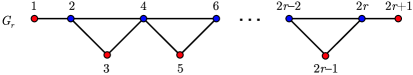
Figure 1: The graph $G_{r}$, with $2r+1$ vertices labeled $i=1,2,\dots,2r+1$.

2.1.4 The graph $\boldsymbol{G_{r}}$

A basic example is the graph $G=G_{r}$ of Fig. 1. It has $2r+1$ vertices and $3r-1$ edges, with the (symmetric) adjacency matrix defined by

$$A_{1,2}=A_{2r,2r+1}=A_{2i,2i+1}=A_{2i,2i+2}=A_{2i+1,2i+2}=1,\qquad i\in\{1,\dots,r-1\}.$$

When $r=0$, $G_{0}$ is reduced to a single vertex labeled $1$, while for $r=1$, $G_{1}$ is a chain of three vertices $1$, $2$, $3$ with the two edges $(1,2)$ and $(2,3)$.

Example 2.1.

The non-vanishing partition functions $Z_{m}^{G_{r}}$ for hard particles on $G_{r}$, $r=0,1$ are

$$Z_{0}^{G_{0}}=1,\qquad Z_{1}^{G_{0}}=y_{1},\qquad Z_{0}^{G_{1}}=1,\qquad Z_{1}^{G_{1}}=y_{1}+y_{2}+y_{3},\qquad Z_{2}^{G_{1}}=y_{1}y_{3}.$$ (2.1)

2.1.5 Recursion relations for the partition function

The transfer matrices $Z_{m}^{G_{r}}$ satisfy recursion relations in the index $r$. They are obtained by considering the possible occupancies of the vertices $2r+1$ and $2r$:

$$Z_{m}^{G_{r}}=Z_{m}^{G_{r-1}}+y_{2r+1}Z_{m-1}^{G_{r-1}}+y_{2r}Z_{m-1}^{G_{r-2}},\qquad r\geq 2,\quad m\geq 0.$$ (2.2)

For example, $Z_{0}^{G_{r}}=1$ is the partition function of the empty configuration and $Z_{r+1}^{G_{r}}=\prod\limits_{i=0}^{r}y_{2i+1}$ for the maximally occupied configuration.

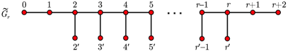
Figure 2: The graph ${\tilde{G}_{r}}$, dual to $G_{r}$, with total of $2r+2$ vertices.

2.2 Transfer matrix on the dual graph

Associated to the graph $G_{r}$, there is a dual graph ${\widetilde{G}}_{r}$, as in Fig. 2.

It is dual in the sense that $G_{r}$ is the medial graph of ${\widetilde{G}}_{r}$: each edge of ${\widetilde{G}}_{r}$ corresponds to a vertex of $G_{r}$, and any two edges of ${\widetilde{G}}_{r}$ share a vertex iff the corresponding vertices of $G_{r}$ are adjacent.

We fix the labeling so that the correspondence is between edges of ${\widetilde{G}}_{r}$ and vertices of $G_{r}$ is:

1. edge $(k,k^{\prime})$ of ${\widetilde{G}}_{r}$ corresponds to the vertex $2k-1$ of $G_{r}$, where $k=2,3,\dots,r$;

2. edge $(k,k+1)$ of ${\widetilde{G}}_{r}$ corresponds to the vertex $2k$ of $G_{r}$, where $k=1,2,\dots,r$;

3. edge $(0,1)$ of ${\widetilde{G}}_{r}$ corresponds to the vertex $1$ of $G_{r}$;

4. edge $(r+1,r+2)$ of ${\widetilde{G}}_{r}$ corresponds to the vertex $2r+1$ of $G_{r}$.

2.2.1 Transfer matrix on $\boldsymbol{\widetilde{G}_{r}}$

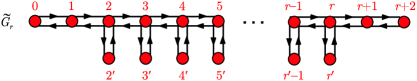
Figure 3: The graph ${\tilde{G}_{r}}$ with oriented edges drawn in.

We choose an ordering of the $2r+2$ vertices of ${\widetilde{G}}_{r}$ to be $0<1<2<2^{\prime}<3<3^{\prime}<\dots<r<r^{\prime}<r+1<r+2$, and consider this to be an index set. We construct the $(2r+2)\times(2r+2)$ transfer matrix $T_{r}(t{\mathbf{y}})$ with these indices. Its entries are $0$ except for:

$$(T_{r})_{k^{\prime},k}=1,\quad(T_{r})_{k,k^{\prime}}=ty_{2k-1},\qquad k=2,3,\dots,r;$$

$$(T_{r})_{k+1,k}=1,\qquad(T_{r})_{k,k+1}=ty_{2k},\qquad k=1,2,\dots,r;$$

$$(T_{r})_{1,0}=(T_{r})_{r+2,r+1}=1,\qquad(T_{r})_{0,1}=ty_{1},\qquad(T_{r})_{r+1,r+2}=ty_{2r+1}.$$

In matrix form,

$$T_{r}(t{\mathbf{y}})=\left(\begin{matrix}0&ty_{1}&0&0&0&\cdots&0&0&0&0\\ 1&0&ty_{2}&0&0&\cdots&0&0&0&0\\ 0&1&0&ty_{3}&ty_{4}&\cdots&0&0&0&0\\ 0&0&1&0&0&\cdots&0&0&0&0\\ 0&0&1&0&0&\cdots&0&0&0&0\\ \vdots&\vdots&&&&\ddots&&&&\vdots\\ 0&0&0&0&0&\cdots&0&ty_{2r-1}&ty_{2r}&0\\ 0&0&0&0&0&\cdots&1&0&0&0\\ 0&0&0&0&0&\cdots&1&0&0&ty_{2r+1}\\ 0&0&0&0&0&\cdots&0&0&1&0\end{matrix}\right).$$ (2.3)

This matrix is a weighted adjacency matrix for the graph $\widetilde{G}_{r}$ as drawn in Fig. 3. Each edge of $\widetilde{G}_{r}$ corresponds to two oriented edges pointing in opposite directions, with the weights in the transfer matrix corresponding to those oriented edges. The element of the transfer matrix indexed by $i$, $j$ is the weight corresponding to the edge $j\to i$.

Lemma 2.2.

The generating function for hard particle partition functions on $G_{r}$ with weights $ty_{i}$ per particle at vertex $i$ is

$$Z^{G_{r}}(t{\mathbf{y}}):=\sum_{m=0}^{r+1}t^{m}Z_{m}^{G_{r}}=\det(I-T_{r}(-t{\mathbf{y}}))$$ (2.4)

with $T_{r}$ as in equation (2.3).

Proof 2.3.

Expanding the determinant $D_{r}(t)=\det(I-T_{r}(-t{\mathbf{y}}))$ along the last column, one obtains the recursion relation:

$$D_{r}(t)=D_{r-1}(t)+ty_{2r+1}D_{r-1}(t)+ty_{2r}D_{r-2}(t),\qquad r\geq 2.$$

Let $D_{r,m}$ denote the coefficient of $t^{m}$ in $D_{r}(t)$. It satisfies the same recursion relation as equation (2.2) for $Z_{m}^{G_{r}}$, with $D_{0}(t)=1+ty_{1}$ and $D_{1}(t)=1+t(y_{1}+y_{2}+y_{3})+t^{2}y_{1}y_{3}$, in agreement with the initial values of $Z^{G_{r}}(t{\mathbf{y}})$, $r=0,1$ in equation (2.1). Thus, $D_{r,m}=Z_{m}^{G_{r}}$ for all $r$, $m$.

Example 2.4.

For the case $r=1$, $G_{1}$ is a chain of 3 vertices $1$, $2$, $3$. The dual ${\widetilde{G}}_{1}$ is a chain of three edges connecting four vertices $0$, $1$, $2$, $3$, and the transfer matrix is:

$$T(t{\mathbf{y}})=\left(\begin{matrix}0&ty_{1}&0&0\\ 1&0&ty_{2}&0\\ 0&1&0&ty_{3}\\ 0&0&1&0\end{matrix}\right).$$

One checks that $\det(I-T(-t{\mathbf{y}}))=1+t(y_{1}+y_{2}+y_{3})+t^{2}y_{1}y_{3}$, in agreement with the partition functions $Z_{i}^{G_{1}}$ of equation (2.1).

2.3 Hard particles and paths

Let $G$ be a graph with oriented edges. For example, the graph $\widetilde{G}_{r}$ of the previous section can be made into an oriented graph, by taking each edge to be a doubly-oriented edge. Then each oriented edge from $i$ to $j$ receives a weight $w(i,j)$, which is the corresponding entry of the transfer matrix $T(t{\mathbf{y}})$ of equation (2.3). This may be interpreted as the transfer matrix for paths on ${\widetilde{G}}_{r}$ as follows.

2.3.1 The partition function of paths

A path of length $n$ on an oriented graph $G$ is a sequence of vertices of $G$, $P=(v_{0},v_{1},\dots,v_{n})$, such that there exists an arrow from $v_{i}$ to $v_{i+1}$ for each $i$. Let $\mathcal{P}_{a,b}^{G}(n)$ be the set of all distinct paths of length $n$, starting at vertex $a$ and ending at vertex $b$ on the graph $G$.

A path on a graph with weighted edges has a total weight which is the product of the weights $w(v_{i},v_{i+1})$ associated with the edges traversed in the path.

The partition function ${\mathcal{Z}}_{a,b}^{G}(n)$ for $\mathcal{P}_{a,b}^{G}(n)$ is

$${\mathcal{Z}}_{a,b}^{G}(n)=\sum_{P\in\mathcal{P}_{a,b}^{G}(n)}\prod_{i=0}^{n-1}w(v_{i},v_{i+1}).$$

Assuming $G$ is finite, and labeling its vertices $i=1,2,\dots,N$, let us introduce the $N\times N$ transfer matrix $T$ with entries $T_{i,j}=w(j,i)$, we have the following simple expression for ${\mathcal{Z}}_{a,b}^{G}(n)$:

$${\mathcal{Z}}_{a,b}^{G}(n)=\big{(}T^{n}\big{)}_{b,a}.$$

The matrix $T(t{\mathbf{y}})$ of (2.3) is then the transfer matrix for paths on ${\widetilde{G}}_{r}$ with weights $1$ for edges pointing away from the vertex $0$, and $ty_{i}$ for the $i$-th edge pointing to the origin. The partition function for weighted paths of arbitrary length on ${\widetilde{G}}_{r}$ from the vertex $0$ to itself is

$${\mathcal{Z}}^{{\widetilde{G}}_{r}}(t{\mathbf{y}})=\sum_{n\geq 0}\big{(}T(t{\mathbf{y}})^{n}\big{)}_{0,0}=\big{(}(I-T(t{\mathbf{y}}))^{-1}\big{)}_{0,0}.$$ (2.5)

Lemma 2.5.

The partition function of paths of arbitrary length from $0$ to $0$ on the graph $\widetilde{G}_{r}$ is equal to

$${\mathcal{Z}}^{{\widetilde{G}}_{r}}(t{\mathbf{y}})={Z^{G_{r}}(0,-ty_{2},\dots,-ty_{2r+1})\over Z^{G_{r}}(-ty_{1},-ty_{2},\dots,-ty_{2r+1})}.$$ (2.6)

Proof 2.6.

By definition, (2.5) is the ratio of the $(0,0)$-minor of the matrix $I-T(t{\mathbf{y}})$ to its determinant. Using equation (2.4) and the explicit form (2.3), this immediately yields the relation.

This relation between hard-particle partition functions and path partition functions may be interpreted as a boson-fermion correspondence, and is a particular case of Viennot’s theory of heaps of pieces [29, 22].

2.3.2 The path partition function as a continued fraction

A direct way to compute ${\mathcal{Z}}^{{\widetilde{G}}_{r}}(t{\mathbf{y}})$ in equation (2.5) is by using Gaussian elimination on $I-T(t{\mathbf{y}})$ to bring it to lower-triangular form. The resulting pivot in the first row is $1/\big{(}(I-T(t{\mathbf{y}}))^{-1}\big{)}_{0,0}$. If we do this systematically, by left-multiplication by upper-triangular elementary matrices, the result is

Lemma 2.7.

$${\mathcal{Z}}^{{\widetilde{G}}_{r}}(t{\mathbf{y}})={1\over 1-t{y_{1}\over 1-t{y_{2}\over 1-ty_{3}-t{y_{4}\over 1-ty_{5}-t{y_{6}\over{\ddots\over 1-ty_{2r-1}-t{y_{2r}\over 1-ty_{2r+1}}}}}}}}.$$ (2.7)

2.3.3 Non-Intersecting paths: the LGV formula

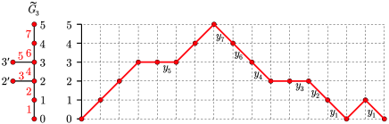
Figure 4: A path on ${\widetilde{G}}_{3}$ with $16$ steps. The weights $y_{i}$ are associated to the descending steps $(1,-1)$ and to the second half of the horizontal steps $(1,0)+(1,0)$ of the path, $i$ being the label of the corresponding edge of ${\widetilde{G}}_{3}$ (see on left). Here, the path receives the weight $y_{1}^{2}y_{2}y_{3}y_{4}y_{5}y_{6}y_{7}$.

We may represent paths of length $2n$ from vertex $0$ to itself on ${\widetilde{G}}_{r}$ as paths on the lattice ${\mathbb{Z}}_{\geq 0}^{2}$ (see Fig. 4 for an illustration). Such paths start at $(0,0)$ and end at $(2n,0)$, and have the following possible steps:

1. to the northeast, $(j,k)\to(j+1,k+1)$, corresponding to the $j$th step in the path going from vertex $k$ to vertex $k+1$;

2. to the southeast, $(j,k)\to(j+1,k-1)$, corresponding to the $j$th step in the path going from vertex $k$ to vertex $k-1$;

3. to the east, $(j,k)\to(j+2,k)$, corresponding to the steps $k\to k^{\prime}\to k$ if $k\in\{2,3,\dots,r\}$.

Paths from the origin to the origin have an even number of steps, by parity.

We will need to consider the partition function of families of ${\alpha}$ non-intersecting paths on $\widetilde{G}_{r}$, ${\mathcal{Z}}_{{\mathbf{s}},{\mathbf{e}}}^{{\widetilde{G}}_{r}}$. Here, the fixed starting points are parametrized by ${\mathbf{s}}=(s_{1},\dots,s_{\alpha})$ and the endpoints by ${\mathbf{e}}=(e_{1},\dots,e_{\alpha})$.

By non-intersecting paths, we mean paths that do not share any vertex. We have the celebrated Lindström–Gessel–Viennot formula [24, 17]

$${\mathcal{Z}}_{{\mathbf{s}},{\mathbf{e}}}^{{\widetilde{G}}_{r}}=\det_{1\leq i,j\leq{\alpha}}\,{\mathcal{Z}}_{s_{i},e_{j}}^{{\widetilde{G}}_{r}}.$$ (2.8)

The determinant has the effect of subtracting the contributions from paths that do intersect. This formula can be proved by expanding the determinant as:

$$\sum_{\sigma\in S_{\alpha}}{\rm sgn}(\sigma)\,\prod_{i=1}^{\alpha}{\mathcal{Z}}_{s_{\sigma(i)},e_{i}}^{{\widetilde{G}}_{r}}.$$ (2.9)

One then considers the involution $\varphi$ on families of paths, defined by interchanging the beginnings of the two first paths that share a vertex until the vertex, or by the identity if no two paths in the family intersect. It is clear that when $\varphi$ does not act as the identity it relates two path configurations with opposite weights in the expansion of the determinant, as the two starting points are switched by $\varphi$, hence these cancel out of the expansion (2.9). We are thus left only with non-intersecting families, all corresponding to $\sigma={\rm Id}$, hence all with positive weights.

3 Application to rank 2 cluster algebras of affine type

3.1 Rank two cluster algebras

In this section, we use the partition functions introduced in the previous section to the problem of computing the cluster variables of rank two cluster algebras of affine type with trivial coefficients. This allows us to give explicit, manifestly positive formulas for the variables, proving the positivity of the variables in these cases.

3.1.1 The recursion relations

The rank 2 cluster algebras of affine type [10, 28] with trivial coefficients may be reduced to the following recursion relations for $n\in{\mathbb{Z}}$:

$$x_{n+1}=\left\{\begin{matrix}\dfrac{1}{x_{n-1}}(1+x_{n}^{b})&{\rm if}\ \ n\ \ {\rm is}\ \ {\rm odd},\vspace{2mm}\\ \dfrac{1}{x_{n-1}}(1+x_{n}^{c})&{\rm if}\ \ n\ \ {\rm is}\ \ {\rm even},\end{matrix}\right.$$ (3.1)

where $b$, $c$ are two positive integers with $bc=4$, hence $(b,c)=(2,2)$, $(4,1)$ or $(1,4)$. The aim is to find an expression for $x_{n}$, $n\in{\mathbb{Z}}$ in terms of some initial data, e.g. $(x_{0},x_{1})$.

The connection to rank 2 affine Lie algebras is via the Cartan matrix $\left(\begin{matrix}2&-b\\ -c&2\end{matrix}\right)$.

The cases $(4,1)$ and $(1,4)$ are almost equivalent: If $x_{n}(x_{0},x_{1})$ is a solution of the $(b,c)$ equation, then $x_{1-n}(x_{1},x_{0})$ is the solution of the $(c,b)$ equation. We may thus restrict ourselves to the $(1,4)$ case.

However, the symmetry $x_{n}\leftrightarrow x_{1-n}$ changes the parity of $n$. Therefore we need to also consider the dependence of $x_{n}$ in the “odd” initial data $(x_{1},x_{2})$.

It turns out that the recursion relations (3.1) are all integrable evolutions. This allows us to compute the generating function for $x_{n}$, $n\geq 0$. The result is a manifestly positive (finite) continued fraction. In the light of the results of the previous section, this allows to reinterpret $x_{n}$ as the partition function for weighted paths on certain graphs. This path formulation gives yet another direct combinatorial interpretation for the expression of $x_{n}$ as a positive Laurent polynomial of the initial data, to be compared with the approach of [28, 6] using quiver representations and that of [26] using matchings of different kinds of graphs.

3.2 The $\boldsymbol{(2,2)}$ case: solution and path interpretation

Consider the recursion relation

$$x_{n+1}x_{n-1}=x_{n}^{2}+1$$ (3.2)

with ${\mathbf{x}}_{0}=(x_{0},x_{1})=(x,y)$. This is the $A_{1}$ case of the renormalized $Q$-system considered in [7].

Due to the symmetry $n\leftrightarrow 1-n$ of the equation, the solution satisfies

$$x_{n}(x_{0},x_{1})=x_{1-n}(x_{1},x_{0})$$

so we may restrict our attention to computing $x_{n}$, for $n\geq 0$.

3.2.1 Constants of the motion

Equation (3.2) is integrable. To see this, we rewrite (3.2) as

$$\varphi_{n}:=\left|\begin{matrix}x_{n-1}&x_{n}\\ x_{n}&x_{n+1}\\ \end{matrix}\right|=1.$$

Then

$$0=\varphi_{n}-\varphi_{n+1}=\left|\begin{matrix}x_{n-1}+x_{n+1}&x_{n}\\ x_{n}+x_{n+2}&x_{n+1}\\ \end{matrix}\right|.$$

We conclude that there exists a constant $c$, independent of $n$, such that $x_{n-1}+x_{n+1}=cx_{n}$ for all $n$. Using equation (3.2),

$$c={x_{n-1}+x_{n+1}\over x_{n}}={x_{n+1}\over x_{n}}+{1\over x_{n}x_{n+1}}+{x_{n}\over x_{n+1}}={x_{1}\over x_{0}}+{1\over x_{0}x_{1}}+{x_{0}\over x_{1}}.$$ (3.3)

We interpret $c$ as an integral of motion of the three-term relation (3.2): all solutions of the latter indeed satisfy the two-term recursion relation (3.3), for some “integration constant” $c$ fixed by the initial data.

Note that $c$ coincides with the partition function $Z_{1}^{G_{1}}=y_{1}+y_{2}+y_{3}$ for one hard particle on the graph $G_{1}$, with weights

$$y_{1}={x_{1}\over x_{0}},\qquad y_{2}={1\over x_{0}x_{1}},\qquad y_{3}={x_{0}\over x_{1}}.$$ (3.4)

Note also that the only other non-vanishing hard particle partition functions on $G_{1}$ are $Z_{0}^{G_{1}}=1$ and $Z_{2}^{G_{1}}=y_{1}y_{3}=1$.

3.2.2 Generating function for $\boldsymbol{x_{n}}$

Let $X(t)=\sum\limits_{n=0}^{\infty}t^{n}x_{n}$ be the generating function for the variables $x_{n}$ with $n\geq 0$. Using $x_{n+1}-cx_{n}+x_{n-1}=0$, we have by direct calculation

$$X(t)={x_{0}-(cx_{0}-x_{1})t\over 1-ct+t^{2}}={x_{0}\over 1-t{y_{1}\over 1-t{y_{2}\over 1-ty_{3}}}},$$ (3.5)

with $y_{i}$ as in (3.4). This gives $x_{n}$ as a manifestly positive Laurent polynomial of $(x_{0},x_{1})$. In fact, expanding the r.h.s. of (3.5), we get

$$X(t)=\sum_{p,q,\ell\geq 0}{p+q-1\choose q}{q+\ell-1\choose\ell}t^{p+q+\ell}x_{0}^{1+\ell-p-q}x_{1}^{p-q-\ell},$$

from which $x_{n}$ is obtained by extracting the coefficient of $t^{n}$. This agrees with the result of [6].

It follows that the dependence of the variables $x_{n}$ on any other pair $(x_{k},x_{k+1})$ is also as a positive Laurent polynomial. This is clear from the translational invariance of the system:

$$x_{n}(x_{k},x_{k+1})=x_{n-k}(x_{0},x_{1})\big{|}_{x_{0}\mapsto x_{k},x_{1}\mapsto x_{k+1}}.$$

3.2.3 Relation to the partition function of paths

Upon comparing the continued fraction expression (3.5) and equation (2.7), we see that there is a path interpretation to the variables $x_{n}$ as follows.

The denominator of the fraction $X(t)$ is equal to the partition function $Z^{G_{1}}(-t{\mathbf{y}})$ for hard particles on the graph $G_{1}$ introduced in Section 2, with the weights $-ty_{i}$ per particle at vertex $i$. Therefore,

$$X(t)=x_{0}\,{Z^{G_{1}}(0,-ty_{2},-ty_{3})\over Z^{G_{1}}(-ty_{1},-ty_{2},-ty_{3})},$$

so $x_{0}^{-1}X(t)$ is equal the partition function for paths on the graph ${\widetilde{G}}_{1}$ of Example 2.4, beginning and ending at the vertex 0. The weights are as follows: The weight is equal to 1 for any step away from vertex 0, and and is equal to $ty_{i}$ per step from vertex $i$ to $i-1$.

3.3 The $\boldsymbol{(1,4)}$ case: solution and relation to paths

We now consider the system:

$$x_{2n}={1+x_{2n-1}\over x_{2n-2}},$$

$$x_{2n+1}={1+x_{2n}^{4}\over x_{2n-1}},\qquad n\in{\mathbb{Z}}.$$

We determine the dependence of the variables $x_{n}$ on two different types of initial conditions:

$${\rm case}\ 0:\ (x_{0},x_{1}),$$

$${\rm case}\ 1:\ (x_{1},x_{2}).$$ (3.6)

We can eliminate the odd variables and get an equation for the even variables. Let $u_{n}=x_{2n}$. Using $x_{2n-1}=u_{n}u_{n-1}-1$, the even variables satisfy the recursion relation

$$u_{n+1}={u_{n}^{3}+u_{n-1}\over u_{n}u_{n-1}-1},$$

or, equivalently, $u_{n}(u_{n+1}u_{n-1}-u_{n}^{2})=u_{n+1}+u_{n-1}$.

3.3.1 Conserved quantities

The variable $w_{n}=u_{n+1}u_{n-1}-u_{n}^{2}$ satisfies

$$w_{n}={u_{n+1}+u_{n-1}\over u_{n}}={u_{n}^{3}+u_{n-1}+(u_{n}u_{n-1}-1)u_{n-1}\over u_{n}(u_{n}u_{-1}-1)}={u_{n}^{2}+u_{n-1}^{2}\over u_{n}u_{n-1}-1}.$$ (3.7)

Moreover,

$$w_{n+1}-w_{n}={u_{n+1}^{2}+u_{n}^{2}\over u_{n+1}u_{n}-1}-{u_{n+1}+u_{n-1}\over u_{n}}={u_{n}^{3}-u_{n+1}u_{n}u_{n-1}+u_{n+1}+u_{n-1}\over u_{n}(u_{n}u_{n+1}-1)}=0.$$

We conclude that $w_{n}$ is a conserved quantity, that is, it is independent of $n$.

Using (3.7), there exists a constant $c$ such that $u_{n+1}+u_{n-1}=cu_{n}$. We may compute this constant explicitly in terms of the initial conditions in cases $0$ and $1$ of (3.6), using $u_{0}=x_{0}$, $u_{1}=x_{2}$ and $x_{0}x_{2}=1+x_{1}$:

$${\rm case}\ 0:\ \ c^{(0)}={u_{1}^{2}+u_{0}^{2}\over u_{1}u_{0}-1}={x_{0}^{2}+x_{2}^{2}\over x_{1}}={x_{0}^{4}+(1+x_{1})^{2}\over x_{0}^{2}x_{1}},$$

$${\rm case}\ 1:\ \ c^{(1)}={x_{2}^{4}+(1+x_{1})^{2}\over x_{2}^{2}x_{1}}.$$

3.3.2 Generating function

The linear recursion relation $u_{n+1}-cu_{n}+u_{n-1}=0$ implies the following formulas for the generating functions

$$U^{(0)}(t):=\sum_{n\geq 0}u_{n}t^{n}={u_{0}-t(c^{(0)}u_{0}-u_{1})\over 1-c^{(0)}t+t^{2}}={x_{0}\over 1-ty^{(0)}_{1}-{t^{2}y^{(0)}_{2}\over 1-ty^{(0)}_{3}}},$$ (3.8)

$$U^{(1)}(t):=\sum_{n\geq 0}u_{n+1}t^{n}={u_{1}-t(c^{(1)}u_{1}-u_{2})\over 1-c^{(1)}t+t^{2}}={x_{2}\over 1-ty_{1}^{(1)}-{t^{2}y^{(1)}_{2}\over 1-ty^{(1)}_{3}}},$$ (3.9)

where the parameters are expressed in terms of the initial data as:

$$y^{(0)}_{1}={1+x_{1}\over x_{0}^{2}},\qquad y^{(0)}_{2}={x_{0}^{4}+(1+x_{1})^{2}\over x_{0}^{4}x_{1}},\qquad y^{(0)}_{3}={x_{0}^{4}+1+x_{1}\over x_{0}^{2}x_{1}},$$

$$y^{(1)}_{1}={x_{2}^{4}+1+x_{1}\over x_{2}^{2}x_{1}},\qquad y^{(1)}_{2}={x_{2}^{4}+(1+x_{1})^{2}\over x_{2}^{4}x_{1}},\qquad y^{(1)}_{3}={1+x_{1}\over x_{2}^{2}}.$$ (3.10)

Note that both sets satisfy the same relation $y^{(i)}_{1}y^{(i)}_{3}=1+y^{(i)}_{2}$ where $i=0,1$, as they are a related via the substitution $x_{2}\leftrightarrow x_{0}$, which maps $\big{(}y^{(1)}_{1},y^{(1)}_{2},y^{(1)}_{3}\big{)}\leftrightarrow\big{(}y^{(0)}_{3},y^{(0)}_{2},y^{(0)}_{1}\big{)}$.

Upon expanding the right hand sides of (3.8) and (3.9) in power series of $t$, we get all the $u_{n}$’s as explicit positive Laurent polynomials of either initial data $(x_{0},x_{1})$ and $(x_{1},x_{2})$. Using

$${1\over 1-ta_{1}-{t^{2}a_{2}\over 1-ta_{3}}}=\sum_{p,q,\ell\geq 0}t^{p+2q+\ell}a_{1}^{p}a_{2}^{q}a_{3}^{\ell}{p+q\choose p}{q+\ell-1\choose\ell}$$

we obtain the expressions, valid for all $n\geq 0$:

$$\hbox{case $0$}:\ \ x_{2n}(x_{0},x_{1})=\sum_{q,\ell,r,s,m\geq 0}x_{0}^{1+4(q+\ell)-2n-4(r+s)}x_{1}^{m-q-\ell}$$

$$\hphantom{\hbox{case $0$}:\ \ x_{2n}(x_{0},x_{1})=}{}\times{n-q-\ell\choose q-r,r}{q+\ell-1\choose\ell-s,s}{n+2r+s-2q-\ell\choose m},$$ (3.11)

$$\hbox{case $1$}:\ \ x_{2n+2}(x_{1},x_{2})=\sum_{q,\ell,r,s,m\geq 0}x_{2}^{1+2n-4(q+\ell+r+s)}x_{1}^{q+\ell+m-n}$$

$$\phantom{\hbox{case $1$}:\ \ x_{2n+2}(x_{1},x_{2})=}{}\times{n-q-\ell\choose q-r,r,s}{q+\ell-1\choose\ell}{2r+s+\ell\choose m},$$ (3.12)

where we have used the multinomial coefficients

$${n\choose m_{1},m_{2},\dots,m_{k}}:=\left\{\begin{array}[]{ll}\dfrac{n!}{m_{1}!\cdots m_{k}!(n-\sum m_{i})!},&\sum_{i}m_{i}\leq n,\vspace{2mm}\\ 0&{\rm otherwise}.\end{array}\right.$$

The expressions for the odd variables follow from $x_{2n+1}=x_{2n}x_{2n+2}-1$. The positivity of these latter expressions is easily checked: Note that the product $x_{2n}x_{2n+2}$ in both equations (3.11) and (3.12) has a constant term $1$ as a Laurent polynomial of $(x_{0},x_{1})$ and $(x_{1},x_{2})$ respectively, hence $x_{2n}x_{2n+2}-1$ is a positive Laurent polynomial.

3.3.3 Path interpretation

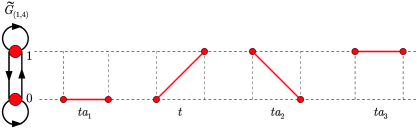
Figure 5: The graph ${\widetilde{G}}_{(1,4)}$ and the four corresponding path steps.

The continued fraction expressions (3.8) and (3.9) allow for a path interpretation of $x_{2n}$ as follows. Consider the graph ${\widetilde{G}}_{(1,4)}$ on the left hand side of Fig. 5, with two vertices labelled $0$, $1$ connected by an edge, and connected to themselves via a loop. We assign weights to the oriented edges as follows:

$$w(0\to 0)=ta_{1},\qquad w(0\to 1)=t,\qquad w(1\to 1)=ta_{3},\qquad w(1\to 0)=ta_{2}.$$

We can also associate a path in ${\mathbb{Z}}_{\geq 0}^{2}$ to a path on $\widetilde{G}_{(1,4)}$ composed of the steps shown in Fig. 5.

The corresponding path transfer matrix is: $T=t\left(\begin{matrix}a_{1}&a_{2}\\ 1&a_{3}\end{matrix}\right)$. Using Gaussian elimination on $I-T$ as in the previous example, we find that the partition function of paths from the vertex 0 to itself is:

$$\big{(}(I-T)^{-1}\big{)}_{0,0}={1\over 1-ta_{1}-{t^{2}a_{2}\over 1-ta_{3}}}.$$

Hence, $x_{2n}$ is (up to a factor of $x_{0}$ in case $0$ and $x_{2}$ in case $1$) the partition function for paths of $2n$ steps on ${\widetilde{G}}_{(1,4)}$, from and to the vertex $0$, with weights $(a_{1},a_{2},a_{3})=(y_{1},y_{2},y_{3})$ in case $(i)$ and $(a_{1},a_{2},a_{3})=(z_{1},z_{2},z_{3})$ in case $(ii)$, where the weights are as in (3.10).

3.3.4 The graph $\boldsymbol{\widetilde{G}_{1,4}}$ as a compactification of the graph $\boldsymbol{\widetilde{G}_{1}}$

We will see later that, quite generally, it is possible to “compactify” the graphs $\widetilde{G}_{r}$. The result for $r=1$ is precisely the graph $\widetilde{G}_{1,4}$. Thus, The case $(b,c)=(2,2)$ of the previous section may also be interpreted in terms of paths on the graph ${\widetilde{G}}_{(1,4)}$, but with different weights:

$$w(0\to 0)=ty_{1},\qquad w(0\to 1)=1,\qquad w(1\to 1)=ty_{3},\qquad w(1\to 0)=ty_{2}.$$

where $y_{i}$ are as in equation (3.4).

To see this, note that the continued fraction (3.5) may be rewritten as:

$$X(t)={x_{0}\over 1-t{y_{1}\over 1-t{y_{2}\over 1-ty_{3}}}}=x_{0}+{tx_{1}\over 1-ty_{1}-{ty_{2}\over 1-ty_{3}}}=x_{0}+tx_{1}\left(\left(I-\left(\begin{matrix}ty_{1}&ty_{2}\\ 1&ty_{3}\end{matrix}\right)\right)^{-1}\right)_{0,0}.$$

Thus, for $n\geq 0$, the solution $x_{n+1}$ of the $(2,2)$ case is up to a factor $x_{1}$ the partition function for paths on ${\widetilde{G}}_{(1,4)}$, from and to the origin vertex $0$, and with a total of $n$ steps of the form $0\to 0$, $1\to 1$ or $1\to 0$, with respective weights $y_{1}$, $y_{2}$, $y_{3}$.

4 Application to the $\boldsymbol{A_{r}}$ $\boldsymbol{Q}$-system

In [19, 7], we showed that the recursion relations ($Q$-systems) satisfied by the characters of the Kirillov–Reshetikhin modules of the quantum affine algebras associated with any simple Lie algebra can be described in terms of mutations of a cluster algebra. Solutions to the cluster algebra recursion relations are more general, in that the initial conditions are not specialized, as they are in the original $Q$-system satisfied by characters of Kirillov–Reshetikhin modules [21].

A particularly simple example of this is the case when the Lie algebra is of type $A$. Characters of $A_{n}$ KR-modules, which are just Schur functions corresponding to rectangular Young diagrams, are given by the cluster variables upon specialization of the boundary conditions. In [8], we gave the general solution for the cluster variables without specialization of initial conditions. For these variables, we proved the positivity conjecture of Fomin and Zelevinsky by mapping the problem to a partition function of weighted paths on a graph. Let us review the results obtained in [8].

4.1 Definition

The $A_{r}$ $Q$-system is the following system of recursion relations for a sequence $R_{{\alpha},n}$, ${\alpha}\in I_{r}=\{1,2,\dots,r\}$ and $n\in{\mathbb{Z}}$:

$$R_{{\alpha},n+1}R_{{\alpha},n-1}=R_{{\alpha},n}^{2}+R_{{\alpha}+1,n}R_{{\alpha}-1,n},$$ (4.1)

with boundary conditions

$$R_{0,n}=R_{r+1,n}=1\qquad\hbox{for all}\ \ n\in{\mathbb{Z}}.$$

We note that the case $r=1$ of $A_{1}$ coincides with the case $(2,2)$ treated in Section 3.2.

Remark 4.1.

The original $Q$-system, which is the one satisfied by the characters of KR-modules, differs from the system (4.1) not only in that it is specialized to the initial conditions $R_{{\alpha},0}=\pm 1$ for all ${\alpha}\in I_{r}$, but also by a minus sign in the second term on the right. In this discussion, we choose to renormalize the variables for simplicity. It is also possible (see the appendix of [7]) to consider the recursion relation with nontrivial coefficients. In that case both (4.1) and the original $Q$-system result from a specialization of the coefficients.

We wish to study the solutions of equation (4.1) for any given initial data. Our standard initial data for the $Q$-system are the variables ${\mathbf{x}}_{0}=(R_{{\alpha},0},R_{{\alpha},1})_{{\alpha}\in I_{r}}$. We may then view equation (4.1) as a three-term recursion relation in $n$, which requires two successive values of $n$ (for each ${\alpha}$) as initial data. Our first goal is to express all $\{R_{{\alpha},n}\}_{{\alpha},n}$ in terms of the initial data ${\mathbf{x}}_{0}$.

4.1.1 Symmetries of the system

We may use equation (4.1) to get both $n\geq 2$ and $n\leq-1$ values in terms of ${\mathbf{x}}_{0}$. These are related via the manifest symmetry of the $Q$-system under $n\leftrightarrow 1-n$, which implies $R_{{\alpha},1-n}\big{(}(R_{{\alpha},0},R_{{\alpha},1})_{{\alpha}\in I_{r}}\big{)}=R_{{\alpha},n}\big{(}(R_{{\alpha},1},R_{{\alpha},0})_{{\alpha}\in I_{r}}\big{)}$. In addition, equation (4.1) is translationally invariant under $n\to n+k$: $R_{{\alpha},n+k}\big{(}(R_{{\alpha},k+1},R_{{\alpha},k})_{{\alpha}\in I_{r}}\big{)}=R_{{\alpha},n}\big{(}(R_{{\alpha},1},R_{{\alpha},0})_{{\alpha}\in I_{r}}\big{)}$ for all $n,k\in{\mathbb{Z}}$.

4.2 Conserved quantities of $\boldsymbol{Q}$-systems as hard particle partition functions

The $Q$-system turns out to be a discrete integrable system, in that it is possible to find a sufficient number of integrals of the motion, as in the $r=1$ case.

First, equation (4.1) may be used to express $R_{{\alpha},n}$ $({\alpha}\geq 2)$ as polynomials in $\{R_{1,n}\}$:

$$R_{{\alpha},n}=\det_{1\leq i,j\leq{\alpha}}\,(R_{1,n+i+j-{\alpha}-1}).$$ (4.2)

This is proved by use of the Desnanot–Jacobi identity for the minors of the $({\alpha}+1)\times({\alpha}+1)$ matrix $M$ with entries $M_{i,j}=R_{1,n+i+j-{\alpha}}$, $i,j\in I_{{\alpha}+1}$.

The boundary condition $R_{r+1,n}=1$ (for all $n$) together with (4.2) implies the equation of motion which determines $R_{1,n}$:

$$\det_{1\leq i,j\leq r+1}(R_{1,n+i+j-r-2})=1.$$

From equation (4.1), it is clear that $R_{r+2,n}=0$ for all $n$. Hence there exists a linear recursion relation of the form

$$\sum_{m=0}^{r+1}(-1)^{m}c_{r+1-m}\,R_{1,n+m}=0,$$ (4.3)

with $c_{0}=c_{r+1}=1$. The fact that $c_{r+1-m}$ do not depend on $n$ follows from the fact that each row in the matrix in the determinant for $R_{r+2,n}$ is just a shift in $n$ of any other row.

The constants $c_{p}$, $p=1,2,\dots,r$ are the $r$ integrals of motion of the $A_{r}$ $Q$-system. They can be expressed explicitly in terms of the $R_{1,n}$s as follows:

$$c_{p}=\det_{1\leq i\leq r+1\atop 1\leq j\leq r+2,\ j\neq r+2-p}\,R_{1,n+i+j-2}$$

independently of $n$. These quantities are similar to those found in [27] for the so-called Coxeter–Toda integrable systems.

By using simple determinant identities, we show in Theorem 3.5 of [8] that $c_{p}$ satisfy recursion relations which allow us to identify them as the partition functions $Z_{p}^{G_{r}}$ of $p$ hard particles on the graph $G_{r}$ of Fig. 1, where the weights given by:

$$y_{2{\alpha}-1,k}={R_{{\alpha}-1,k}R_{{\alpha},k+1}\over R_{{\alpha},k}R_{{\alpha}-1,k+1}},\quad 1\leq{\alpha}\leq r+1,\qquad y_{2{\alpha},k}={R_{{\alpha}-1,k}R_{{\alpha}+1,k+1}\over R_{{\alpha},k}R_{{\alpha},k+1}},\quad 1\leq{\alpha}\leq r.\!\!$$ (4.4)

This is true for any $k$: The functions $Z_{p}^{G_{r}}$ are independent of the choice of $k$. Thus, unless otherwise stated, $y_{\alpha}$ will stand for $y_{{\alpha},0}$ below.

4.3 $\boldsymbol{Q}$-system solutions and paths

The linear recursion relation (4.3) allows to compute the generating function $R^{(r)}(t)=\sum\limits_{n=0}^{\infty}t^{n}R_{1,n}$ explicitly. Indeed, $R^{(r)}(t)Z^{G_{r}}(-t{\mathbf{y}})$ is a polynomial of degree $r$, and it is easy to see that

$$R^{(r)}(t)Z^{G_{r}}(-t{\mathbf{y}})=R_{1,0}Z^{G_{r}}(0,-ty_{2},\dots,-ty_{2r+1}).$$

Using (2.6), we may interpret $R^{(r)}(t)/R_{1,0}$ as the generating function ${\mathcal{Z}}_{0,0}^{{\widetilde{G}}_{r}}(t{\mathbf{y}})$ for paths on ${\widetilde{G}}_{r}$ with the weights (4.4), say for $k=0$. In other words, $R_{1,n}/R_{1,0}$ is the partition function for weighted paths of $2n$ steps on ${\widetilde{G}}_{r}$ starting and ending at the origin (or starting at $(0,0)$ and ending at $(2n,0)$ in the two-dimensional representation).

Comparing the determinant formula for $R_{{\alpha},n}$ (4.2) and the LGV formula (2.8) for families of ${\alpha}$ non-intersecting paths, we have [8]

Lemma 4.2.

The quantity $R_{{\alpha},n}/(R_{1,0})^{\alpha}$ is the partition function ${\mathcal{Z}}_{{\mathbf{s}},{\mathbf{e}}}^{{\widetilde{G}}_{r}}$ for ${\alpha}$ non-intersecting weighted paths on ${\widetilde{G}}_{r}$ with starting and ending points $s_{i}=(2i-2,0)$, $e_{i}=(2n+2{\alpha}-2i,0)$, $i=1,2,\dots,{\alpha}$.

Proof 4.3.

It is clear that ${\mathcal{Z}}_{s_{i},e_{j}}^{{\widetilde{G}}_{r}}$ is the partition function for paths from $(2i-2,0)$ to $(2n+2{\alpha}-2j,0)$, which is equal to that from $(0,0)$ to $(2(n+{\alpha}+1-i-j),0)$ by translational invariance. This allows to identify the two determinants (4.2) and (2.8), up to an overall factor of $(R_{1,0})^{\alpha}$, and the result follows.

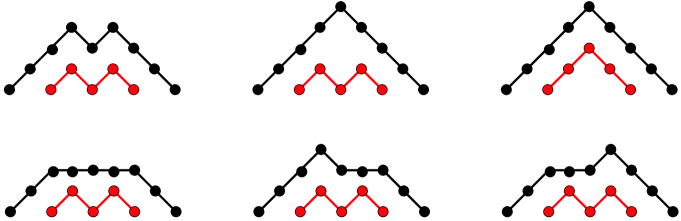
Figure 6: The six pairs of non-intersecting paths on ${\widetilde{G}}_{2}$ of $8$ and $4$ steps, starting respectively at $(0,0)$ and $(2,0)$ and ending at $(6,0)$ and $(8,0)$.

As an illustration, we have represented in Fig. 6 the six pairs of non-intersecting paths contributing to $R_{2,3}$, solution of the $A_{2}$ $Q$-system.

Thus, we have proved

Theorem 4.4.

The variables $R_{{\alpha},n}$ which satisfy (4.1), when expressed in terms of the variables ${\mathbf{x}}_{0}$, are equal to $(R_{1,0})^{\alpha}$ times partition functions for paths on the graph $\widetilde{G}_{r}$, involving only the weights $y_{\alpha}$ of (4.4). These weights are explicit Laurent monomials of the initial data ${\mathbf{x}}_{0}=(R_{{\alpha},0},R_{{\alpha},1})_{{\alpha}\in I_{r}}$. This gives an explicit expression for $R_{{\alpha},n}$ as Laurent polynomials of the initial data, with non-negative integer coefficients.

4.4 An alternative path formulation

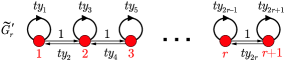
Figure 7: The graph ${\widetilde{G}}_{r}^{\prime}$, with $r+1$ vertices. We have indicated the weights attached to each oriented edge.

In the same spirit as Section 3.3.4, one can show (see below) that the solution $R_{1,n}$ of the $A_{r}$ $Q$-system may also be interpreted in terms of paths on a new (“compactified”) graph ${\widetilde{G}}^{\prime}_{r}$ of Fig. 7. This is a graph with $r+1$ vertices, labelled $1,2,\dots,r+1$, connected via oriented edges $i\to i+1$, $i+1\to i$, $i=1,2,\dots,r$ and loops $i\to i$, $i=1,2,\dots,r+1$.

To each edge is attached a weight as follows:

$${\rm wt}(i\to i+1)=1,\qquad{\rm wt}(i+1\to i)=ty_{2i},\qquad{\rm wt}(i\to i)=ty_{2i-1}.$$ (4.5)

The corresponding transfer matrix encoding these weights is an $(r+1)\times(r+1)$-matrix of the form

$$T^{\prime}=\left(\begin{matrix}ty_{1}&ty_{2}&0&\cdots&\cdots&\cdots&\cdots&0\\ 1&ty_{3}&ty_{4}&0&&&&\vdots\\ 0&1&ty_{5}&ty_{6}&0&&&\vdots\\ \vdots&\ddots&\ddots&\ddots&\ddots&\ddots&&\vdots\\ \vdots&&\ddots&\ddots&\ddots&\ddots&\ddots&\vdots\\ \vdots&&&0&1&ty_{2r-3}&ty_{2r-2}&0\\ \vdots&&&&0&1&ty_{2r-1}&ty_{2r}\\ 0&\cdots&\cdots&\cdots&\cdots&0&1&ty_{2r+1}\end{matrix}\right).$$ (4.6)

Then we have

$${R^{(r)}(t)\over R_{1,0}}=1+t{y_{1}\over 1-ty_{1}-t{y_{2}\over 1-ty_{3}-t{y_{4}\over 1-ty_{5}-t{y_{6}\over{\ddots\over 1-ty_{2r-1}-t{y_{2r}\over 1-ty_{2r+1}}}}}}}$$

$$\hphantom{{R^{(r)}(t)\over R_{1,0}}}{}=1+t{R_{1,1}\over R_{1,0}}\big{(}(I-T^{\prime})^{-1}\big{)}_{1,1}.$$ (4.7)

This is readily proved by Gaussian elimination.

Comparing this expression to the results of the previous section, we conclude that

Lemma 4.5.

For $n\geq 0$, $R_{1,n+1}/R_{1,1}$ is the partition function for paths on the weighted graph ${\widetilde{G}}^{\prime}_{r}$, with a total of $n$ steps along the edges of type $i\to i$ or $i+1\to i$ in ${\widetilde{G}}^{\prime}_{r}$, starting and ending at vertex $1$.

The weights are given in equation (4.5) with $y_{i}$ as in (4.4) with $k=0$.

In Section 7 we will relate this result to the total positivity conjecture of Fomin and Zelevinsky and networks.

We may actually write an explicit expression for $R_{1,n}$ by simply expanding the continued fraction (4.7) as:

$$R^{(r)}(t)=R_{1,0}\Bigg{(}1+ty_{1}\sum_{p_{1},p_{2},\dots,p_{2r+1}\geq 0\atop p_{0}=p_{2r+2}=0}\prod_{\ell=0}^{r}(ty_{2\ell+1})^{p_{2\ell+1}}$$

$$\phantom{R^{(r)}(t)=}{}\times(ty_{2\ell+2})^{p_{2\ell+2}}{p_{2\ell}+p_{2\ell+1}+p_{2\ell+2}-1\choose p_{2\ell}-1,p_{2\ell+1}}\Bigg{)}.$$

Substituting the values (4.4) for the weights $y_{{\alpha}}\equiv y_{{\alpha},0}$, and extracting the coefficient of $t^{n+1}$, we get for all $n\geq 0$:

$$R_{1,n+1}=R_{1,1}\sum_{p_{1},p_{2},\dots,p_{2r+1}\geq 0\atop p_{0}=p_{2r+2}=0,\ \Sigma p_{i}=n}\prod_{i=1}^{r}{(R_{i,0})^{p_{2i+2}+p_{2i+1}-p_{2i}-p_{2i-1}}\over(R_{i,1})^{p_{2i+1}+p_{2i}-p_{2i-1}-p_{2i-2}}}\prod_{\ell=0}^{r}{p_{2\ell}+p_{2\ell+1}+p_{2\ell+2}-1\choose p_{2\ell}-1,p_{2\ell+1}}$$

as explicit positive Laurent polynomials of the initial data. This gives a rank-$r$ generalization of the formula given in [6] for $r=1$.

5 Cluster algebra formulation: mutations and paths
for the $\boldsymbol{A_{r}}$ $\boldsymbol{Q}$-system

In this section, we show that the solutions $\{R_{{\alpha},n}\ |\ {\alpha}\in I_{r},n\in{\mathbb{Z}}\}$ of the $Q$-system are positive Laurent polynomials when expressed as functions of an arbitrary set initial conditions. This generalizes our result for the initial condition ${\mathbf{x}}_{0}$ in the previous section.

The recursion relation (4.1) has a solution once a certain set of initial conditions is specified, but this set need not necessarily be the set ${\mathbf{x}}_{0}$. We will explain below that the most general possible choice of initial conditions is specified by a Motzkin path of length $r$.

The solutions of (4.1) can be viewed as cluster variables in the $A_{r}$ $Q$-system cluster algebra defined in [19]. Hence, our proof provides a general confirmation of the conjecture of [10] for this particular cluster algebra: When the cluster variables are expressed as functions of the variables in any other cluster (i.e. an arbitrary set of initial conditions), they are Laurent polynomials with non-negative coefficients.

The results of this sections were explained in detailed in [8], and this section should serve as a summary of the proofs contained therein.

5.1 The $\boldsymbol{Q}$-system as cluster algebra

In [19], it was shown that the $A_{r}$ $Q$-system solutions $\{R_{{\alpha},n}\}$ may be viewed as a subset of the cluster variables of the $A_{r}$ $Q$-system cluster algebra. This is a cluster algebra with trivial coefficients, which includes the the seed cluster variable $(R_{1,0},R_{2,0},\dots,R_{r,0},R_{1,1},R_{2,1},\dots,R_{r,1})$, with an associated associated $2r\times 2r$ exchange matrix has the block form: $\begin{pmatrix}0&-C\\ C&0\end{pmatrix}$, $C$ the Cartan matrix of $A_{r}$.

In this language, each cluster is a vector with $2r$ variables, and the subset of clusters relevant to the $Q$-system are those which have entries made up entirely of solutions to the $Q$-system (we restrict to these in the following). These clusters are all related by sequences of cluster mutations which are one of the relations (4.1).

Because of the form of equation (4.1), it is easy to see that the restricted set of clusters corresponding to the $Q$-system are characterized by a set of $r$ integers $(m_{1},\dots,m_{r})$, subject to the condition that $|m_{\alpha}-m_{{\alpha}+1}|\leq 1$. This defines what is known as a Motzkin path.

Definition 5.1.

The cluster ${\mathbf{x}}_{{\mathbf{m}}}$ corresponding to the set of integers ${\mathbf{m}}=(m_{1},\dots,m_{r})$ is the vector of $2r$ variables $\{R_{{\alpha},m_{\alpha}},R_{{\alpha},m_{\alpha}+1}\}_{{\alpha}\in I_{r}}$, ordered so that all variables with an even second index appear first.

For example, the initial cluster ${\mathbf{x}}_{0}$ corresponds to the Motzkin path ${\mathbf{m}}=(0,0,\dots,0)$, and ${\mathbf{x}}_{0}=(R_{1,0},\dots,R_{r,0},R_{1,1},\dots,R_{r,1})$.

For any ${\mathbf{m}}$, ${\mathbf{x}}_{\mathbf{m}}$ is obtained from the fundamental initial seed ${\mathbf{x}}_{0}$ by mutations of the cluster algebra. This is just saying that one gets ${\mathbf{x}}_{\mathbf{m}}$ by repeated selected applications of the recursion relation (4.1) to ${\mathbf{x}}_{0}$. Each mutation changes only one of the cluster variables. That is, for some ${\alpha}$ and $n$,

$$R_{{\alpha},n}\mapsto\left\{\begin{array}[]{ll}R_{{\alpha},n+2}=\frac{R_{{\alpha},n+1}^{2}+R_{{\alpha}+1,n+1}R_{{\alpha}-1,n+1}}{R_{{\alpha},n}}&\hbox{(forward mutation at ${\alpha}$)},\\ R_{{\alpha},n-2}=\frac{R_{{\alpha},n-1}^{2}+R_{{\alpha}+1,n-1}R_{{\alpha}-1,n-1}}{R_{{\alpha},n}}&\hbox{(backward mutation at ${\alpha}$)}.\end{array}\right.$$

Recall that we only consider here particular mutations that only involve solutions of the $Q$-system. Here we have used the “time” variable $n$ to define forward (resp. backward) mutations according to whether the mutation increases (resp. decreases) the index $n$ in the mutated cluster variable.

Alternatively, the mutation changes the Motzkin path which characterizes ${\mathbf{x}}_{\mathbf{m}}$, by changing ${\mathbf{m}}\mapsto{\mathbf{m}}\pm\epsilon_{{\alpha}}$, with the plus (minus) sign for a forward (backward) mutation. Here, $\epsilon_{{\alpha}}$ is the vector which is zero except for the entry ${\alpha}$, which is equal to 1. We see that accordingly the Motzkin path locally moves forward (backward).

The Laurent property of cluster algebras ensures that every cluster variable is a Laurent polynomial of the cluster variables of any other cluster in the algebra.

The positivity property, proved only in particular cases so far, is that these Laurent polynomials have non-negative integer coefficients. The property was proved for the particular clusters considered in the present case in [8]. It may be stated as follows:

Theorem 5.2 ([8]).

Each $R_{{\alpha},n}$, when expressed as a function of the seed ${\mathbf{x}}_{\mathbf{m}}$ for any Motzkin path ${\mathbf{m}}$, is a Laurent polynomial of $\{R_{{\alpha},m_{\alpha}},R_{{\alpha},m_{\alpha}+1}\;|\;{\alpha}\in I_{r}\}$, with non-negative integer coefficients.

We outline the proof below.

For clarity let us introduce the following notation. Let $F$ be some cluster variable. Then $F$ can be expressed as a function of ${\mathbf{x}}_{\mathbf{m}}$ for any ${\mathbf{m}}$. The functional form is then denoted by $F=F_{\mathbf{m}}({\mathbf{x}}_{\mathbf{m}})$. Since $F$ can also be expressed as a function of any other cluster, we can write $F_{\mathbf{m}}({\mathbf{x}}_{\mathbf{m}})=F_{{\mathbf{m}}^{\prime}}({\mathbf{x}}_{{\mathbf{m}}^{\prime}})$ for any two Motzkin paths ${\mathbf{m}}$, ${\mathbf{m}}^{\prime}$. In particular, in the notation of the previous section, we have $R^{(r)}(t)=R^{(r)}_{{\mathbf{m}}_{0}}(t;{\mathbf{x}}_{0})$.

5.2 Target graphs and weights

Due to the reflection and translation symmetries of the $Q$-system, we can restrict our attention to seeds associated with Motzkin paths in a fundamental domain $\mathcal{M}_{r}=\{{\mathbf{m}}\ |\ {\rm min}_{\alpha}(m_{\alpha})=0\}$. There are $3^{r-1}$ elements in $\mathcal{M}_{r}$.

To each Motzkin path ${\mathbf{m}}\in{\mathcal{M}}_{r}$, we associate a pair $(\Gamma_{\mathbf{m}},\{y_{e}({\mathbf{m}})\})$, consisting of a rooted graph $\Gamma_{\mathbf{m}}$ with oriented edges, and edge weights $y_{e}({{\mathbf{m}}})$ along the edges $e$.

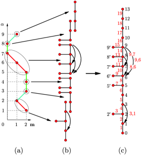
Figure 8: The Motzkin path ${\mathbf{m}}=(2,1,2,2,2,1,0,0,1)$ for $r=9$ (a) is decomposed into $p=6$ descending segments $(12)(3)(4)(567)(8)(9)$ (circled, red edges). The corresponding graph pieces $\Gamma_{{\mathbf{m}}_{i}}$ are indicated in (b). They are to be glued “horizontally” for flat transitions (green edges) and “vertically” for ascending ones (blue edges). The resulting graph $\Gamma_{\mathbf{m}}$ is represented (c) with its vertex (black) and edge (red) labels.

5.2.1 Construction of the graph $\boldsymbol{\Gamma_{\mathbf{m}}}$

The graph $\Gamma_{\mathbf{m}}$ is constructed via the following sequence of steps (see Fig. 8 for an illustration):

1. Decompose the Motzkin path ${\mathbf{m}}$ into maximal “descending segments” ${\mathbf{m}}_{i}$ of length $k_{i}$ ($i=1,\dots,p$). These are segments of the form ${\mathbf{m}}_{i}=(m_{{\alpha}_{i}},m_{{\alpha}_{i}+1},\dots,m_{{\alpha}_{i+1}-1})$ with $\alpha_{i+1}=\alpha_{i}+k_{i}$, where $m_{{\alpha}_{i}+j}=m_{{\alpha}_{i}}-j$. Here, ${\alpha}_{1}=1$ and ${\alpha}_{p+1}-1=r$.

2. The separation between two consecutive descending segments of the Motzkin path, ${\mathbf{m}}_{i}$ and ${\mathbf{m}}_{i+1}$ is either “flat” i.e. $m_{{\alpha}_{i+1}}=m_{{\alpha}_{i+1}-1}$ or “ascending” i.e. $m_{{\alpha}_{i+1}}=m_{{\alpha}_{i+1}-1}+1$.

3. To each descending segment ${\mathbf{m}}_{i}$, associate a graph $\Gamma_{{\mathbf{m}}_{i}}$, which is the graph ${\widetilde{G}}_{k_{i}}$ with additional, down-pointing edges $a\to b$ for all $a$, $b$ such that $k_{i}+1\geq a>b+1\geq 2$. There are a total of $k_{i}(k_{i}-1)/2$ extra oriented edges.

4. We glue the graphs $\Gamma_{{\mathbf{m}}_{i}}$ and $\Gamma_{{\mathbf{m}}_{i+1}}$ into a graph $\Gamma_{{\mathbf{m}}_{i}}||\Gamma_{{\mathbf{m}}_{i+1}}$ defined as follows (see Fig. 8 for an illustration):

   1. If the separation between ${\mathbf{m}}_{i}$ and ${\mathbf{m}}_{i+1}$ is flat, we identify vertex $0$ of $\Gamma_{{\mathbf{m}}_{i+1}}$ with vertex $k_{i}+2$ of $\Gamma_{{\mathbf{m}}_{i}}$, and vertex $1$ of $\Gamma_{{\mathbf{m}}_{i+1}}$ with vertex $k_{i}+1$ of $\Gamma_{{\mathbf{m}}_{i}}$, while the connecting edges are identified.

   2. If the separation is ascending, we reverse the role of vertices $0$ and $1$ in the procedure above.

The result of this procedure is the graph $\Gamma_{\mathbf{m}}=\Gamma_{{\mathbf{m}}_{1}}||\Gamma_{{\mathbf{m}}_{2}}||\cdots||\Gamma_{{\mathbf{m}}_{p}}$. Its root is the vertex $0$ of $\Gamma_{{\mathbf{m}}_{1}}$.

We label the vertices of the graph $\Gamma_{\mathbf{m}}$ by the integers $i$ with $i\in\{0,\dots,r+2+n_{+}({\mathbf{m}})\}$ (where $n_{+}({\mathbf{m}})$ is the number of $m_{\alpha}$ such that $m_{{\alpha}+1}=m_{\alpha}+1$) and labels $i^{\prime}$ for any univalent vertex attached to vertex $i$ via a horizontal edge. We do this by labeling the vertices of $\Gamma_{\mathbf{m}}$ from bottom to top, by shifting the labels of the subgraphs $\Gamma_{{\mathbf{m}}_{i}}$ so that no label is skipped nor repeated.

The edges $e$ pointing towards the root of $\Gamma_{\mathbf{m}}$ are of two types:

1. the “skeleton edges” belonging to some ${\widetilde{G}}_{k_{i}}$ in the above construction;

2. the extra, down-pointing edges added in the gluing procedure.

5.2.2 The weights on the graph $\boldsymbol{\Gamma_{\mathbf{m}}}$

We label the $2r+1$ skeleton edges of type $(i)$ by ${\alpha}=1,2,\dots,2r+1$ from bottom to top (see the example in Fig. 8), and the weights are denoted by $y_{\alpha}({\mathbf{m}})$. Weights assigned to edges pointing away from the root are all set to 1.

Alternatively, we may label the “down pointing” skeleton edges by the pairs of vertices $i+1\to i$ or $i^{\prime}\to i$ which they connect. The extra edges of type $(ii)$ are also labeled by the pairs $a\to b$ of vertices which they connect. All edge weights may be labeled by the label of the edge.

The weights of the edges of type $(ii)$ can be expressed in terms of the skeleton weights:

$$y_{a,b}({\mathbf{m}})={\prod\limits_{b\leq i<a}y_{i+1,i}({\mathbf{m}})\over\prod\limits_{b<i<a}y_{i^{\prime},i}({\mathbf{m}})},$$

so that they obey the following intertwining condition

$$y_{a,b}({\mathbf{m}})y_{a^{\prime},b^{\prime}}({\mathbf{m}})=y_{a,b^{\prime}}({\mathbf{m}})y_{a^{\prime},b}({\mathbf{m}}),\qquad a>a^{\prime}>b>b^{\prime}.$$ (5.1)

For example, the extra weights of the example of Fig. 8 read respectively: $y_{3,1}=y_{2}y_{4}/y_{3}$, $y_{9,7}=y_{14}y_{12}/y_{13}$, $y_{8,6}=y_{12}y_{10}/y_{11}$, and $y_{9,6}=y_{9,7}y_{8,6}/y_{12}=y_{14}y_{12}y_{10}/(y_{13}y_{11})$.

Finally, for a given Motzkin path ${\mathbf{m}}\in{\mathcal{M}}_{r}$, we define the skeleton weights $y_{\alpha}({\mathbf{m}})$, ${\alpha}=1,2,\dots,2r+1$ to be:

$$y_{2{\alpha}-1}({\mathbf{m}})={\lambda_{{\alpha},m_{\alpha}}\over\lambda_{{\alpha}-1,m_{{\alpha}-1}}},\qquad{\alpha}=1,2,\dots,r+1,$$ (5.2)

$$y_{2{\alpha}}({\mathbf{m}})={\mu_{{\alpha}+1,m_{\alpha}+1}\over\mu_{{\alpha},m_{{\alpha}}}}\left(1-\delta_{m_{\alpha},m_{{\alpha}+1}+1}+{\lambda_{{\alpha}+1,m_{{\alpha}+1}}\over\lambda_{{\alpha}+1,m_{{\alpha}}}}\delta_{m_{\alpha},m_{{\alpha}+1}+1}\right)$$

$$\phantom{y_{2{\alpha}}({\mathbf{m}})=}{}\times\left(1-\delta_{m_{{\alpha}-1},m_{{\alpha}}+1}+{\lambda_{{\alpha}-1,m_{{\alpha}}}\over\lambda_{{\alpha}-1,m_{{\alpha}-1}}}\delta_{m_{{\alpha}-1},m_{{\alpha}}+1}\right),\qquad{\alpha}=1,2,\dots,r,$$ (5.3)

where

$$\lambda_{{\alpha},n}={R_{{\alpha},n+1}\over R_{{\alpha},n}},\qquad\mu_{{\alpha},n}={R_{{\alpha},n}\over R_{{\alpha}-1,n}}.$$

Note that with these definitions the expressions (5.2), (5.3) involve only variables of the seed ${\mathbf{x}}_{\mathbf{m}}$.

To each Motzkin path ${\mathbf{m}}\in{\mathcal{M}}_{r}$, we may finally associate a transfer matrix $T_{\mathbf{m}}\equiv T_{\mathbf{m}}(t{\mathbf{y}}({\mathbf{m}}))$, with entries $(T_{\mathbf{m}})_{b,a}=$ weight of the oriented edge $a\to b$ on $\Gamma_{\mathbf{m}}$. Then the series in $t$

$$\mathcal{Z}_{\mathbf{m}}(t;{\mathbf{x}}_{\mathbf{m}}):=\big{(}(I-T_{{\mathbf{m}}})^{-1}\big{)}_{0,0}=\sum_{n}t^{n}\mathcal{Z}_{0,0}^{\Gamma_{{\mathbf{m}}}}(n)$$ (5.4)

is the generating function for weighted paths on $\Gamma_{\mathbf{m}}$, with the coefficient of $t^{n}$ being the partition function of walks from vertex 0 to itself on $\Gamma_{\mathbf{m}}$ which have $n$ down-pointing steps. When ${\mathbf{m}}={\mathbf{m}}_{0}=\mathbf{0}$, this coincides with  (2.5).

5.3 Mutations, paths and continued fraction rearrangements

Our purpose is to write an explicit expression for the functional dependence of the variables $R_{{\alpha},n}$ on the seed variable ${\mathbf{x}}_{\mathbf{m}}$, that is, find $(R_{{\alpha},n})_{{\mathbf{m}}}({\mathbf{x}}_{\mathbf{m}})$ for each ${\alpha}$, $n$ and a Motzkin path ${\mathbf{m}}$.

To do this, we will describe how the generating function $R^{(r)}(t)=R^{(r)}_{{\mathbf{m}}}(t;{\mathbf{x}}_{{\mathbf{m}}})$ is related to the generating function $R^{(r)}_{{\mathbf{m}}^{\prime}}(t;{\mathbf{x}}_{{\mathbf{m}}^{\prime}})$, where ${\mathbf{m}}$ and ${\mathbf{m}}^{\prime}$ are related by a mutation. Then we start from the known function $R_{{\mathbf{m}}_{0}}^{(r)}(t;{\mathbf{x}}_{{\mathbf{m}}_{0}})$, and apply mutations to obtain all other functions $R^{(r)}_{{\mathbf{m}}}$ with ${\mathbf{m}}$ in the fundamental domain $\mathcal{M}_{r}$.

One can cover the entire fundamental domain $\mathcal{M}_{r}$ starting from ${\mathbf{m}}_{0}=\mathbf{0}$ by using only forward mutations ${\mathbf{m}}\mapsto{\mathbf{m}}^{\prime}={\mathbf{m}}+\epsilon_{\alpha}$ of either type $(i)$ $(\dots,a,a,a+1,\dots)\mapsto(\dots,a,a+1,a+1,\dots)$ and $(ii)$ $(\dots,a,a,a,\dots)\mapsto(\dots,a,a+1,a,\dots)$, with the obvious truncations when ${\alpha}=1$ or $r$. (See Remark 8.1 in [8].)

Suppose ${\mathbf{m}}$ and ${\mathbf{m}}^{\prime}$ are related by such a mutation. We compute the two generating functions of the type (5.4), $\mathcal{Z}_{\mathbf{m}}(t;{\mathbf{x}}_{\mathbf{m}})$ and $\mathcal{Z}_{{\mathbf{m}}^{\prime}}(t;{\mathbf{x}}_{{\mathbf{m}}^{\prime}})$.

In fact, the two matrices, $T_{{\mathbf{m}}}$ and $T_{{\mathbf{m}}^{\prime}}$ differ only locally, so that in computing the two generating functions by row reduction, we find that the calculation differs only in a finite number of steps. Note that generating functions take the form of finite continued fractions with manifestly positive series expansions of $t$.

We note two simple rearrangement lemmas which can be used to relate finite continued fractions:

$${(R_{1})}\quad{1\over 1-{a\over 1-b}}=1+{a\over 1-a-b},$$

$${(R_{2})}\quad a+{b\over 1-c}={a^{\prime}\over 1-{b^{\prime}\over 1-c^{\prime}}},\quad\hbox{where}\ \ a^{\prime}=a+b,\ \ b^{\prime}={bc\over a+b},\ \ c^{\prime}={ac\over a+b}.$$

One checks this by explicit calculation.

Let ${\alpha}>1$. Then, using $(R_{2})$ we can show that $\mathcal{Z}_{\mathbf{m}}(t;{\mathbf{x}}_{\mathbf{m}})=\mathcal{Z}_{{\mathbf{m}}^{\prime}}(t;{\mathbf{x}}_{{\mathbf{m}}^{\prime}})$ if and only if the weights $y_{i}\equiv y_{i}({\mathbf{m}})$ and $y_{i}^{\prime}\equiv y_{i}({\mathbf{m}}^{\prime})$ are related via:

$$(i)\ m_{{\alpha}-1}=m_{\alpha}<m_{{\alpha}+1}:\quad y_{\beta}^{\prime}=\left\{\begin{array}[]{ll}y_{2{\alpha}-1}+y_{2{\alpha}},&\beta=2{\alpha}-1,\\ y_{2{\alpha}}y_{2{\alpha}+1}/(y_{2{\alpha}-1}+y_{2{\alpha}}),&\beta=2{\alpha},\\ y_{2{\alpha}-1}y_{2{\alpha}+1}/(y_{2{\alpha}-1}+y_{2{\alpha}}),&\beta=2{\alpha}+1,\\ y_{\beta},&\hbox{otherwise},\end{array}\right.$$

$$(ii)\ m_{{\alpha}-1}=m_{\alpha}=m_{{\alpha}+1}:\quad y_{\beta}^{\prime}=\left\{\begin{array}[]{ll}y_{2{\alpha}-1}+y_{2{\alpha}},&\beta=2{\alpha}-1,\\ y_{2{\alpha}}y_{2{\alpha}+1}/(y_{2{\alpha}-1}+y_{2{\alpha}}),&\beta=2{\alpha},\\ y_{2{\alpha}-1}y_{2{\alpha}+1}/(y_{2{\alpha}-1}+y_{2{\alpha}}),&\beta=2{\alpha}+1,\\ y_{2{\alpha}+2}y_{2{\alpha}-1}/(y_{2{\alpha}-1}+y_{2{\alpha}}),&\beta=2{\alpha}+2,\\ y_{\beta},&\hbox{otherwise}.\end{array}\right.$$

One checks directly that the expressions (5.2), (5.3) indeed satisfy the above relations.

The boundary case, where ${\alpha}=1$, is treated analogously, but first requires a “rerooting” of the graph to its vertex $1$, which is implemented by the application of $(R_{1})$: Indeed, we simply write $\mathcal{Z}_{{\mathbf{m}}}(t;{\mathbf{x}}_{\mathbf{m}})=\big{(}(I-T_{\mathbf{m}})^{-1}\big{)}_{0,0}=1+ty_{1}({\mathbf{m}})\mathcal{Z}^{\prime}_{\mathbf{m}}(t;{\mathbf{x}}_{{\mathbf{m}}})$ with $\mathcal{Z}_{\mathbf{m}}^{\prime}(t;{\mathbf{x}}_{\mathbf{m}})=\big{(}(I-T_{\mathbf{m}})^{-1}\big{)}_{1,1}$. We then rearrange $\mathcal{Z}_{\mathbf{m}}^{\prime}(t;{\mathbf{x}}_{{\mathbf{m}}})$ using $(R_{2})$ again, and find that $\mathcal{Z}_{{\mathbf{m}}}^{\prime}(t;{\mathbf{x}}_{\mathbf{m}})=\mathcal{Z}_{{\mathbf{m}}^{\prime}}(t;{\mathbf{x}}_{{\mathbf{m}}^{\prime}})$ if and only if the weights are related via the above equations.

The net result is the following. Given a compound mutation $\mu_{\mathbf{m}}$ which maps the fundamental Motzkin path ${\mathbf{m}}_{0}$ to ${\mathbf{m}}=(m_{\alpha})_{{\alpha}\in I_{r}}$, then there are exactly $m_{1}$ “rerootings” as described above. This corresponds to rewriting the generating function

$$R^{(r)}_{\mathbf{m}}(t;{\mathbf{x}}_{\mathbf{m}})=\sum_{i=0}^{m_{1}-1}t^{i}R_{1,i}+t^{m_{1}}R_{1,m_{1}}\mathcal{Z}_{{\mathbf{m}}}(t;{\mathbf{x}}_{\mathbf{m}})$$

with $\mathcal{Z}_{{\mathbf{m}}}(t;{\mathbf{x}}_{\mathbf{m}})$ as in equation (5.4).

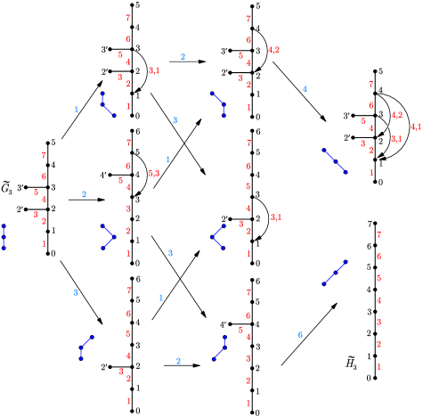
Figure 9: The Motzkin paths ${\mathbf{m}}$ of the fundamental domain ${\mathcal{M}}_{3}$ and the associated graphs $\Gamma_{\mathbf{m}}$, with their vertex and edge labels. We have also indicated the mutations by arrows, the label being ${\alpha}$ when the mutation $\mu_{\alpha}$ acts on variables $R_{{\alpha},m}$ with an even index $m$ and ${\alpha}+r$ for an odd index $m$.

This leads to the following main result:

Theorem 5.3.

For each $n\geq 0$, the function $(R_{1,n+m_{1}})_{\mathbf{m}}({\mathbf{x}}_{\mathbf{m}})=R_{1,m_{1}}\,{\mathcal{Z}}_{0,0}^{\Gamma_{\mathbf{m}}}(n)$. Thus it is proportional to the generating function for weighted paths on the graph $\Gamma_{\mathbf{m}}$ with positive weights, so it is a manifestly positive Laurent polynomial of the initial data ${\mathbf{x}}_{\mathbf{m}}$.

We have represented in Fig. 9 the graphs $\Gamma_{\mathbf{m}}$ for the Motzkin paths ${\mathbf{m}}$ of the fundamental domain ${\mathcal{M}}_{r}$ for $r=3$.

5.4 $\boldsymbol{Q}$-system solutions as strongly non-intersecting paths

To treat the case of $R_{{\alpha},n}$ with ${\alpha}\neq 1$, given a Motzkin path ${\mathbf{m}}\in{\mathcal{M}}_{r}$, we need a path interpretation for the determinant formula for $R_{{\alpha},n+m_{1}}$:

$${R_{{\alpha},n+m_{1}}\over(R_{1,m_{1}})^{\alpha}}={\det\left(R_{1,n+m_{1}+i+j-{\alpha}-1}\right)_{1\leq i,j\leq{\alpha}}\over R_{1,n+m_{1}}}=\det\left({\mathcal{Z}}_{0,0}^{\Gamma_{\mathbf{m}}}(n+i+j-{\alpha}-1)\right)_{1\leq i,j\leq{\alpha}}.$$ (5.5)

Here, we have used the result of the previous section to rewrite the formula in terms of the partition function for paths on $\Gamma_{\mathbf{m}}$, from and to the root, and with $n+i+j-{\alpha}-1$ down steps. As in the standard LGV formula, we interpret this determinant as a certain partition function for paths on $\Gamma_{\mathbf{m}}$ starting from the root at times $0,2,4,\dots,2{\alpha}-2$ and ending at the origin at times $2n,2n+2,\dots,2n+2{\alpha}-2$.

Figure 10: The two-dimensional representation of a typical path on the graph $\Gamma_{\mathbf{m}}$, ${\mathbf{m}}$ the strictly descending Motzkin path $(2,1,0)$ of the case $A_{3}$. Descents of $h=2$ are vertical (time displacement by $2-h=0$), while descents of $h=3$ go back one step in time (time displacement by $2-h=-1$). With these choices, the total time distance between start and end is twice the number of descents ($16=2\times 8$ here).

5.4.1 Paths on $\boldsymbol{\Gamma_{\mathbf{m}}}$ represented as paths on a square lattice

We draw paths, with allowed steps dictated by the graph $\Gamma_{\mathbf{m}}$, on a square-lattice in two dimensions. Paths start and end at $y$-coordinate $0$. Moreover, if a path has $n$ “down” steps (steps towards the vertex 0), then its starting and ending point are separated by $2n$ horizontal steps. That is, a path is from $(x,0)$ to $(x+2n,0)$ where $x$ the starting time and $n$ is the number of down-steps.

Since the horizontal distance between the starting and ending points is fixed by the number of “down” steps, a single step of the form

$$a\to b=a-h$$

should have a horizontal displacement $2-h$ (instead of 1 as in the usual case). That is, on the square lattice it is a segment of the form

$$(x,a)\to(x+2-h,a-h).$$

Some examples are illustrated in Fig. 10.

Thus, we identify ${\mathcal{Z}}_{0,0}^{\Gamma_{\mathbf{m}}}(n+i+j-{\alpha}-1)={\mathcal{Z}}_{s_{i},e_{j}}^{\Gamma_{\mathbf{m}}}$ with paths on the two-dimensional lattice starting at the point $s_{i}=(2i-2,0)$ and ending at the point $e_{j}=(2n+2{\alpha}-2j,0)$, with the types of steps allowed given by the edges of $\Gamma_{\mathbf{m}}$ in the way explained in the previous paragraph.

5.4.2 Strongly non-intersecting paths

We now look at families of ${\alpha}$ paths, corresponding to the determinant in equation (5.5). Such paths may have crossing on the lattice. As in the case of LGV formula, the determinant cancels out contributions from paths which share a vertex. However, other situations may occur: Two paths may cross without sharing a vertex in our picture.

One can generalize the proof of the LGV formula to take such crossings into account. Using the expansion (2.9), and introducing an involution $\varphi$ on families of paths. This involution interchanges the beginnings of the first two paths which share a vertex or which cross each other, by transforming the crossing segments $[P,Q]$ and $[R,S]$ into non-crossing ones $[R,Q]$ and $[P,S]$. This effectively interchanges the two paths up to the points $P$ and $R$ respectively, whichever comes first.

As in the usual case, the involution $\varphi$ acts as the identity if no two paths cross, share a vertex, or can be made to cross via such an exchange.

Taking into account the weights of the paths, the intertwining condition (5.1) implies that the flip preserves the absolute value of the weight, but changes its sign, due to the transposition of starting points. So the determinant (5.5) cancels not only the paths that share a vertex or that cross, but also those that come “too close” to one-another, namely that can be made to cross via a flip.

We call the families of paths which are invariant under the involution $\varphi$ strongly non-intersecting paths.

To summarize, we have the following theorem:

Theorem 5.4.

For any Motzkin path ${\mathbf{m}}\in\mathcal{M}_{r}$, the variable $R_{{\alpha},n+m_{1}}$ $($with $n+m_{1}\geq{\alpha}-1)$ is equal to $(R_{1,m_{1}})^{\alpha}$ times the partition function of ${\alpha}$ strongly non-intersecting paths with steps and weights determined by $\Gamma_{\mathbf{m}}$. The starting points are $s_{i}=(2i-2,0)$ and the end points are $e_{j}=(2n+2{\alpha}-2j,0)$, with $i,j=1,\dots,{\alpha}$, and the weights are functions of the cluster ${\mathbf{x}}_{\mathbf{m}}$.

In particular, $(R_{{\alpha},n+m_{1}})_{\mathbf{m}}({\mathbf{x}}_{\mathbf{m}})$ is a Laurent polynomial with non-negative coefficients of the cluster ${\mathbf{x}}_{\mathbf{m}}$.

6 A new path formulation for the $\boldsymbol{A_{r}}$ $\boldsymbol{Q}$-system

In Section 5, we constructed a set of transfer matrices $T_{\mathbf{m}}$, associated with paths on the graphs $\Gamma_{\mathbf{m}}$, which allowed us to interpret $R_{1,n}$ as generating functions of weighted paths on a graph $\Gamma_{\mathbf{m}}$, and hence prove their positivity as a function of the seed variables ${\mathbf{x}}_{\mathbf{m}}$.

In Section 4.4, we also showed that for the special case ${\mathbf{m}}={\mathbf{m}}_{0}=\mathbf{0}$, there is an alternative graph $\Gamma^{\prime}_{{\mathbf{m}}_{0}}=\widetilde{G}_{r}^{\prime}$, and that one can interpret $R_{1,n}$ as a generating function for paths this alternative “compactified” graph. The graph $\Gamma^{\prime}_{{\mathbf{m}}_{0}}$ has $r+1$ vertices, hence the associated transfer matrix is of size $r+1\times r+1$.

We now ask the question, is there a corresponding compactified set of graphs, $\Gamma_{\mathbf{m}}^{\prime}$, which give a path formulation of $R_{1,n}$ with weights which given by functions of the seed ${\mathbf{x}}_{\mathbf{m}}$ for all Motzkin paths in $\mathcal{M}_{r}$?

It turns out that it is always possible to find a weighted graph with $r+1$ vertices which answers this question positively for each ${\mathbf{m}}$. This corresponds to a set of transfer matrices of a size equal to the rank of the algebra $A_{r}$. Therefore this transfer matrix allows us to make a direct connection between our transfer matrix approach and the totally positive matrices of [14].

6.1 Compactified graphs

Consider the collection of graphs $\Gamma_{\mathbf{m}}$. If we are interested in the generating function of weighted paths on them from the vertex $0$ to itself, then we can make various changes in them locally (“compactify” them) without affecting the generating function itself.

We obtain such compactified graphs from $\Gamma_{\mathbf{m}}$ by identifying pairs of neighboring vertices, and, when necessary, adding oriented edges to cancel unwanted terms. There are two possible ways to make such identifications. Before presenting the general case, let us illustrate the two situations in the following subsection.

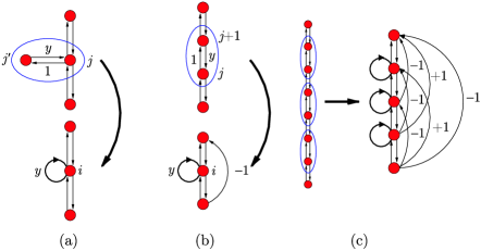
Figure 11: The identification of horizontal (a) or vertical (b) pairs of consecutive vertices on $\Gamma_{\mathbf{m}}$ and the result on $\Gamma_{\mathbf{m}}^{\prime}$. The new edge on $\Gamma_{\mathbf{m}}^{\prime}$ with weight $-1$ allows to subtract the contribution from paths that do not exist on $\Gamma_{\mathbf{m}}$. We have also represented the situation of a longer chain (c), where the identification now requires a network of up-pointing edges with alternating weights $\pm 1$ for the suitable subtractions.

6.2 Examples of compactification

In fact, the first type of compactification, applied to $\widetilde{G}_{r}$, leads to the alternative graph $\widetilde{G}_{r}^{\prime}$ obtained in Section 4.4. Recall that the generating function for paths from $1$ to $1$ on the graph $\widetilde{G}_{r}$ of Fig. 3 is related to the generating function for paths from $0$ to $0$ via the rerooting procedure:

$$\mathcal{Z}_{0,0}^{\widetilde{G}_{r}}=1+ty_{1}\times\mathcal{Z}_{1,1}^{\widetilde{G}_{r}}.$$

Example 6.1.

The generating function $\mathcal{Z}_{1,1}^{\widetilde{G}_{r}}$ is equal to the generating function of paths from $1$ to $1$ on the graph obtained from $\widetilde{G}_{r}$ via the following procedure (“compactification”):

1. Identifying vertex $i^{\prime}$ with vertex $i$, whenever both exist, and attaching a loop with weight $ty_{i^{\prime},i}$ to the resulting vertex (see Fig. 11 (a)).

2. Identifying vertex $r+2$ with vertex $r+1$, and attaching a loop with weight $ty_{r+2,r+1}$ to the resulting vertex.

3. Identifying vertex $1$ with vertex $0$, renaming the resulting vertex $1$, and attaching a loop with weight $ty_{1}=ty_{1,0}$ to this vertex.

This is clear, since a path from $1$ to $1$ through the vertex $i^{\prime}$ must have a segment $i\to i^{\prime}\to i$ with weight $ty_{i^{\prime},i}$, and if it goes through the vertex $r+2$ it must have a segment $r+1\to r+2\to r+1$ with weight $ty_{r+2,r+1}$. Similarly, the loop at $1$ accounts for segments of the form $1\to 0\to 1$.

Note that the resulting graph is $\widetilde{G}_{r}^{\prime}$ of Fig. 7. Thus, we have the identity of Section 4.4

$$\mathcal{Z}_{1,1}^{\widetilde{G}_{r}}=\mathcal{Z}_{1,1}^{\widetilde{G}_{r}^{\prime}}.$$

Another example of identification of vertices is the case when the two vertices are adjacent vertices, $(i,i+1)$, on the spine of $\Gamma$ (see Fig. 11 (b)).

Example 6.2.

Consider the graph $\widetilde{H}_{k}$ associated to an ascending Motzkin path segment of length $k$ (see the example for $k=3$ in the lower right hand corner of Fig. 9). This is a vertical chain of $2k+2$ vertices, numbered from $0$ to $2k+1$ from bottom to top, connected by edges oriented in both directions. The edges $i+1\to i$ have weights $y_{i+1}$ and the edges $i\to i+1$ have weights 1.

Suppose we identify the vertices $a,a+1$ in this graph for some $a$. A path from $0$ to $0$ with a step $a\to a+1$ is always paired with a step $a+1\to a$, for a net contribution to the weight of the path of $y_{a+1}$. We associate a loop with weight $y_{a+1}$ at the newly formed vertex after the identification of vertices $a$ and $a+1$.

However, there are “forbidden” paths on the resulting graph, paths which are not inherited from paths on $\widetilde{H}_{r}$. These are paths which go from $a+2\to a-1$ without traversing the loop. This would correspond to going from $a+2$ to $a-1$ on $\widetilde{H}_{r}$ without passing through the edge $a+1\to a$, which is impossible. We cancel the contribution of these paths by adding an ascending edge $a-1\to a+2$ with weight $-1$. The effect is precisely to subtract the weights of the forbidden set of paths.

More generally, a succession of identifications of the type in the example above results in the following (see Fig. 11 (c)):

Lemma 6.3.

The generating function of paths from $0$ to $0$ on the graph $\widetilde{H}_{k}$ with vertices $0,\dots,2k+1$ is equal to the generating function for paths from $0$ to $0$ on the following compactified graph $\widetilde{H}^{\prime}_{k}$:

1. Identify the vertices $2i+1$ and $2i+2$; rename the resulting vertex $i+1$ $(i=0,\dots,k-1)$.

2. Attach a loop at the vertex $i+1$ with weight $w_{i+1}=y_{2i+2}$. Other edge weights remain unchanged.

3. Add ascending edges $j\to j+2+a$ $(0\leq a\leq k-1-j$, $0\leq j\leq k-1)$ with weight $(-1)^{a+1}$ to the resulting graph.

An illustration of the resulting graph $\widetilde{H}^{\prime}_{k}$ is given in (c) of Fig. 11.

Proof 6.4.

Consider the set of paths $\mathcal{P}$ of the form $P_{1}P^{+}P_{2}P^{-}P_{3}$, where $P_{i}$ are fixed paths, and $P^{+}$ is a path from $h_{0}$ to $h_{1}$ consisting of only up steps and loop steps, and $P^{-}$ is a path from $h_{1}$ to $h_{0}$ consisting only of down steps and loop steps. We furthermore restrict ourselves to paths with the weight($P^{+}$)$\times$ weight($P^{-}$) fixed to be ${\mathbf{y}}\mathbf{w}^{\mathbf{n}}=w_{1}^{n_{1}}\cdots w_{k}^{n_{k}}$ for some ${\mathbf{n}}$. Here, ${\mathbf{y}}$ is the product of the weights of the down steps in $P^{-}$, and ${\mathbf{w}}^{\mathbf{n}}$ is the total weight coming from the loops in the path. Let $f$ be the weight of the remaining fixed portions of the path.

Without loss of generality, we can take $h_{0}=0$ and $h_{1}=k+1$.

For each such path we can decompose $n_{i}=n_{i}^{+}+n_{i}^{-}$, where $n_{i}^{+}$ is the number of times the loop with weight $w_{i}$ is traversed in $P^{+}$, and $n_{i}^{-}$ in $P^{-}$. Paths which arise from paths on $\widetilde{H}_{k}$ must have $n_{i}^{-}\geq 1$ (for all $i$) by definition. We claim that on $\widetilde{H}^{\prime}_{k}$, paths with $n_{i}^{-}=0$ are cancelled by paths which pass through the new ascending edges.

The key observation is that a path which has an up step going through the ascending oriented edge $i-1\to i+a+1$ ($a\geq 0$) on $\widetilde{H}^{\prime}_{k}$ has $n_{i}^{+}=n_{i+1}^{+}=\cdots=n_{i+a}=0$.

Then the total contribution of the paths in $\mathcal{P}$ to the partition function is in fact

$$f{\mathbf{y}}\sum_{n_{i}^{+}+n_{i}^{-}=n_{i}\atop n_{i}^{-}>0}\mathbf{w}^{\mathbf{n}}=f{\mathbf{y}}\sum_{n_{i}^{+}+n_{i}^{-}=n_{i}\atop n_{i}^{+}>0}\mathbf{w}^{\mathbf{n}}$$

$$\hphantom{f{\mathbf{y}}\sum_{n_{i}^{+}+n_{i}^{-}=n_{i}\atop n_{i}^{-}>0}\mathbf{w}^{\mathbf{n}}}{}=f{\mathbf{y}}\sum_{n_{i}^{+}+n_{i}^{-}=n_{i}}\mathbf{w}^{\mathbf{n}}-f{\mathbf{y}}\sum_{j=1}^{k}\sum_{n_{i}^{+}+n_{i}^{-}=n_{i}\atop n_{j}^{+}=0}\mathbf{w}^{\mathbf{n}}$$

$$\hphantom{f{\mathbf{y}}\sum_{n_{i}^{+}+n_{i}^{-}=n_{i}\atop n_{i}^{-}>0}\mathbf{w}^{\mathbf{n}}=}{}+f{\mathbf{y}}\sum_{j_{1}<j_{2}}\sum_{n_{j_{1}}^{+}=n_{j_{2}}^{+}=0}\mathbf{w}^{\mathbf{n}}-f{\mathbf{y}}\sum_{j_{1}<j_{2}<j_{3}}\sum_{n_{j_{1}}^{+}=n_{j_{2}}^{+}=n_{j_{3}}^{+}=0}\mathbf{w}^{\mathbf{n}}+\cdots$$

$$\hphantom{f{\mathbf{y}}\sum_{n_{i}^{+}+n_{i}^{-}=n_{i}\atop n_{i}^{-}>0}\mathbf{w}^{\mathbf{n}}}{}=f{\mathbf{y}}\sum_{a=0}^{k}(-1)^{a}\sum_{j_{1}<\cdots<j_{a}}\sum_{n_{j_{1}}^{+}=\cdots=n^{+}_{j_{a}}=0}\mathbf{w}^{{\mathbf{n}}}.$$

So the alternating sum has the effect of subtracting the terms with any $n_{i}^{-}=0$.

A path on the graph $\widetilde{H}^{\prime}_{k}$ with $a$ spine vertices skipped (by traversing ascending edges of length $>1$) comes with a total sign $(-1)^{x}$ where $x=\sum(\hbox{length of the ascending segments}-1)=a$. That is also the sign of the term with $n_{j_{1}}^{+}=\cdots=n_{j_{a}}^{+}=0$ in the summation.

Finally, we note that any path can be decomposed into pairs of ascending and descending segments as above, and the proof can be applied iteratively to any path.

6.3 Definition of compactified graphs

On a graph $\Gamma_{\mathbf{m}}$, we call a skeleton edge horizontal if it connects (a) vertices $i$ and $i^{\prime}$ for some $i$, (b) vertices $0$ and $1$, or (c) the top vertex and the one below it. We call an edge vertical otherwise.

Definition 6.5.

The compactified graph $\Gamma_{{\mathbf{m}}}^{\prime}$ with $r+1$ vertices is obtained from the graph $\Gamma_{\mathbf{m}}$ via the following compactification procedure:

1. Introduce an order on the vertices of $\Gamma_{\mathbf{m}}$, so that $i<i+1$ and $i<i^{\prime}<i+1$. Number them from $1$ to $2r+2$ accordingly.

2. Identify vertices $2j-1$, $2j$ ($j=1,\dots,r+1$), and rename the resulting vertex $j$. Double edges connecting $(2j-1,2j)$ are replaced by a loop at $j$ with weight which is the product of the weights on the two edges. All other edges and their weights are unchanged.

3. All maximal subgraphs of the form $\widetilde{H}_{k}$ of $\Gamma_{{\mathbf{m}}}$, consisting of vertical edges only, are replaced by compactified weighted graphs of the form $\widetilde{H}_{k}^{\prime}$, as in Lemma 6.3 (with the obvious shift in labels).

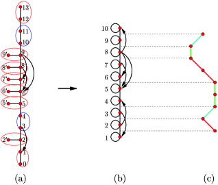
Figure 12: (a) The graph $\Gamma_{\mathbf{m}}$ of Fig. 8, and (b) the compacted graph $\Gamma_{\mathbf{m}}^{\prime}$. We have circled on $\Gamma_{\mathbf{m}}$ the pairs of vertices to be identified in the compactification procedure (in red for horizontal pairs, in blue for vertical pairs). We also represent in (c) the Motzkin path ${\mathbf{m}}$.

Example 6.6.

For illustration, the identification of edges in the case of the graph of Fig. 8 (c) are: $0\sim 1$, $2\sim 2^{\prime}$, $3\sim 4$, $5\sim 5^{\prime}$, $6\sim 6^{\prime}$, $7\sim 7^{\prime}$, $8\sim 8^{\prime}$, $9\sim 9^{\prime}$, $10\sim 11$ and $12\sim 13$. See Fig. 12. There are two maximal subgraphs of the form $\widetilde{H}_{1}$ are the vertices $2$, $3$, $4$, $5$ and $9$, $10$, $11$, $12$. Each pair now corresponds to a vertex $i$ in $\Gamma_{\mathbf{m}}^{\prime}$, $i=1,2,\dots,10$, which receives a loop $i\to i$ from the identification.

Fig. 13 shows the set of compactified graphs corresponding to Fig. 9 for the case $A_{3}$.

The resulting weighted graph $\Gamma_{\mathbf{m}}^{\prime}$ has $r+1$ vertices labelled $1,2,\dots,r+1$, and hence is associated with a transfer matrix $T_{\mathbf{m}}^{\prime}$ of size $r+1\times r+1$.

6.4 An alternative construction

An alternative description of the compactified graphs $\Gamma^{\prime}_{\mathbf{m}}$ is the following.

We start from the graph $\Gamma_{{\mathbf{m}}_{0}}^{\prime}\equiv{\widetilde{G}}_{r}^{\prime}$ of Fig. 7. The loop at vertex $i$ has weight $ty_{2i-1}$ and the edge $i+1\to i$ has weight $ty_{2i}$, where $y_{j}=y_{j}({\mathbf{m}}_{0})$ are as in equations (5.2), (5.3).

Decompose ${\mathbf{m}}$ into maximal segments of the form:

1. descending segments, $D_{{\alpha},i}=(({\alpha},m),({\alpha}+1,m-1),\dots,({\alpha}+i-1,m-i+1))$;

2. ascending segments, $A_{{\alpha},i}=(({\alpha},m),({\alpha}+1,m+1),\dots,({\alpha}+i-1,m+i-1))$;

3. flat segments $(({\alpha},m),({\alpha}+1,m),\dots,({\alpha}+k-1,m))$.

Here, $i\geq 2$ and $k\geq 1$.

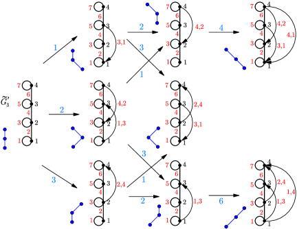
Figure 13: The Motzkin paths ${\mathbf{m}}$ of the fundamental domain ${\mathcal{M}}_{3}$ and the associated compact graphs $\Gamma_{\mathbf{m}}^{\prime}$, with their vertex and edge labels. Note the up-step weights: $y_{1,3}=y_{2,4}=-1$ and $y_{1,4}=1$. Mutations are indicated by arrows.

Definition 6.7.

The graph $\Gamma_{\mathbf{m}}^{\prime\prime}$ is the graph obtained from $\Gamma_{{\mathbf{m}}_{0}}^{\prime}=\widetilde{G}_{r}^{\prime}$ via the following steps:

1. For each descending sequence $D_{{\alpha},i}$ we add descending edges ${\alpha}+p\to{\alpha}+q$ ($0<q+1<p\leq i$) to $\Gamma_{{\mathbf{m}}_{0}}^{\prime}$, with weights $ty_{{\alpha}+p,{\alpha}+q}({\mathbf{m}})$, where

   $$y_{{\alpha}+p,{\alpha}+q}({\mathbf{m}})={\prod\limits_{j={\alpha}+q}^{{\alpha}+p-1}y_{2j}({\mathbf{m}})\over\prod\limits_{j={\alpha}+q+1}^{{\alpha}+p-1}y_{2j-1}({\mathbf{m}})}.$$ (6.1)

2. For each ascending sequence $A_{{\alpha},i}$, we add ascending edges ${\alpha}+q\to{\alpha}+p$ ($0<q+1<p\leq i$) with weights $y_{{\alpha}+q,{\alpha}+p}({\mathbf{m}})=(-1)^{p-q-1}$.

Lemma 6.8.

The weighted graph $\Gamma^{\prime\prime}_{\mathbf{m}}$ is identical to the weighted graph $\Gamma^{\prime}_{\mathbf{m}}$.

This is just the result of the definition of $\Gamma_{\mathbf{m}}$ using the decomposition of ${\mathbf{m}}$, as in Fig. 8. Maximal subgraphs the form $\widetilde{H}_{k}$ correspond to the maximal ascending segments of the Motzkin path. All other segments correspond to subgraphs with horizontal edges.

6.5 Equality of generating functions

To summarize, the compactified graph $\Gamma^{\prime}_{\mathbf{m}}$ is such that

Theorem 6.9.

$$(1-T_{{\mathbf{m}}})^{-1}_{1,1}=(1-T_{{\mathbf{m}}}^{\prime})^{-1}_{1,1}.$$

In other words: the partition function for weighted paths from vertex $1$ to vertex $1$ in $\Gamma_{{\mathbf{m}}}$ is identical to that for weighted paths from vertex $1$ to vertex $1$ in the compact graph $\Gamma_{\mathbf{m}}^{\prime}$.

7 Totally positive matrices and compactified transfer matrices

We now establish the connection between the transfer matrices $T^{\prime}_{\mathbf{m}}$ for paths on $\Gamma^{\prime}_{\mathbf{m}}$ and the totally positive matrices of [14] corresponding to double Bruhat cells for pairs of Coxeter elements.

We may express the compact transfer matrices $T_{\mathbf{m}}^{\prime}$ of the previous section in terms of the elementary matrices $f_{i}$, $e_{i}$, $d_{i}$ for $GL_{r+1}$, defined as follows. Let $E_{ij}$ denote the standard elementary matrix of size $(r+1)\times(r+1)$, with entries $(E_{i,j})_{k,\ell}=\delta_{k,i}\delta_{\ell,j}$.

Definition 7.1.

The elementary matrices $\{e_{i},f_{i},d_{i}\}$ are defined by

$$f_{i}=I+\lambda_{i}E_{i+1,i},\qquad e_{i}=I+\nu_{i}E_{i,i+1},\qquad i\in\{1,\dots,r\},$$

$$d_{i}=I+(\mu_{i}-1)E_{i,i},\qquad i\in\{1,\dots,r+1\}.$$ (7.1)

for some real parameters $\lambda_{i}$, $\mu_{i}$, $\nu_{i}$.

In [14], Fomin and Zelevinsky introduced a parametrization of totally positive matrices as products of the form $\prod\limits_{i\in I}f_{i}\prod\limits_{i=1}^{r+1}d_{i}\prod\limits_{j\in J}e_{j}$ for $I$, $J$ two suitable sets of indices, and $\lambda_{i}$, $\mu_{i}$, $\nu_{i}$ some positive parameters. This expression allowed to rephrase total positivity in terms of networks. Here we interpret our compact transfer matrices in terms of some of these products.

Recall that each Motzkin path can be decomposed into descending, ascending and flat pieces, as in Section 6.4. We introduce the increasing sequence of integers $(a_{1},\dots,a_{2k})$, such that the $j$th ascending piece of ${\mathbf{m}}$, $A_{{{\alpha}_{j}},i_{j}}$ of ${\mathbf{m}}$ starts at $m_{{\alpha}_{j}}=a_{2j-1}$ and ends at $m_{{{\alpha}_{j}}+i_{j}-1}=a_{2j}$. Similarly for the sequence of increasing integers $(b_{1},\dots,b_{2p})$, which mark the starting and ending points of the descending sequences $D_{{\alpha}_{j},i}$.

For $i<j$, let $\omega[i,j]$ denote the permutation which reverses the order of all consecutive elements between $i$ and $j$ in a given sequence. That is, $\omega[i,j]=(i,j)(i+1,j-1)(i+2,j-2)\cdots$. For example, $\omega[i,j]$: $(j,j-1,\dots,i)\mapsto(i,i+1,\dots,j)$,

$$\sigma_{\mathbf{m}}=\left(\prod_{i=1}^{k}\omega[a_{2i-1},a_{2i}]\right)\circ(r,r-1,\dots,1),$$

$$\tau_{{\mathbf{m}}}=\left(\prod_{i=1}^{p}\omega[b_{2i-1},b_{2i}]\right)\circ(r,r-1,\dots,1).$$ (7.2)

Example 7.2.

For the Motzkin path ${\mathbf{m}}=(2,1,2,2,2,1,0,0,1)$ of Fig. 8, we have the ascending segments $[2,3]$ and $[8,9]$, while the descending segments are $[1,2]$ and $[5,7]$. The rearranged sequences read $\sigma_{\mathbf{m}}=(8,9,7,6,5,4,2,3,1)$ and $\tau_{\mathbf{m}}=(9,8,5,6,7,4,3,1,2)$.

Note that the sequences $\sigma_{\mathbf{m}}$ and $\tau_{\mathbf{m}}$ consist of increasing and decreasing subsequences of consecutive integers, and that these subsequences and their order are unique.

One can define the decomposition of the transfer matrix $T_{\mathbf{m}}^{\prime}$ into a strictly lower-triangular part $N_{\mathbf{m}}$ and an upper triangular part $B_{\mathbf{m}}$, so that

$$T_{{\mathbf{m}}}^{\prime}=N_{{\mathbf{m}}}+B_{\mathbf{m}}.$$

Lemma 7.3.

The matrices $N_{\mathbf{m}}$ and $B_{\mathbf{m}}$ can be expressed as

$$N_{\mathbf{m}}=I-(f_{i_{1}}f_{i_{2}}\cdots f_{i_{r}})^{-1},$$ (7.3)

$$B_{\mathbf{m}}=t(d_{1}d_{2}\cdots d_{r+1})\,(e_{j_{1}}e_{j_{2}}\cdots e_{j_{r}}),$$ (7.4)

where the parameters in equation (7.1) are

$$\lambda_{i}=1,\qquad\mu_{i}=y_{2i-1},\qquad\nu_{i}={y_{2i}\over y_{2i-1}}.$$ (7.5)

Proof 7.4.

We give a pictorial proof. It is possible to describe multiplication by an elementary matrix as the addition of an arrow to a graph. In our context, $N_{\mathbf{m}}$ encodes the ascending arrows in the graph $\Gamma_{\mathbf{m}}^{\prime}$, and $B_{\mathbf{m}}$ the descending arrows.

First, consider the product $f_{i_{r}}^{-1}\cdots f_{i_{1}}^{-1}$ in $N_{\mathbf{m}}$ of equation (7.3), where $(f_{i})^{-1}=I-E_{i+1,i}$.

The sequence $(i_{r},i_{r-1},\dots,i_{1})=\big{(}\prod_{i}\omega[a_{2i-1},a_{2i}]\big{)}\circ(1,\dots,r)$, which is simply $\sigma_{\mathbf{m}}$ written in reverse order, consists of alternating increasing and decreasing sequences of consecutive integers. The products of matrices corresponding to increasing subsequences are

$$P^{+}_{j}=f^{-1}_{a_{2j}+1}f^{-1}_{a_{2j}+2}\cdots f^{-1}_{a_{2j+1}-1}=I-\sum_{i=1}^{a_{2j+1}-a_{2j}-1}E_{a_{2j}+i+1,a_{2j}+i}$$

and products corresponding to decreasing sequences are

$$P^{-}_{j}=f^{-1}_{a_{2j}}f^{-1}_{a_{2j}-1}\cdots f^{-1}_{a_{2j-1}}=I+\sum_{i=1}^{a_{2j}-a_{2j-1}}\sum_{k=0}^{i-1}(-1)^{i+k}E_{a_{2j-1}+i,a_{2j-1}+k}.$$

We start with the graph corresponding to the identity matrix, which is the transfer matrix of the graph consisting of $r+1$ disconnected vertices labelled $1,2,\dots,r+1$, each with a loop of weight $1$. Multiplying on the left by $f_{j}^{-1}$ creates an ascending edge $j\to j+1$ with weight $-1$. More generally, left multiplication by $P^{+}_{j}$ creates a succession of ascending edges $a_{2j}+1\to a_{2j}+2$, $a_{2j}+2\to a_{2j}+3$, …, $a_{2j+1}-1\to a_{2j+1}$. Left multiplication by $P^{-}_{j}$ creates a web of ascending edges $a_{2j-1}+k\to a_{2j-1}+i$, $0\leq k\leq i-1\leq a_{2j}-a_{2j-1}-1$, with alternating weights $(-1)^{i+k}$. We illustrate the resulting actions on the graphs in Fig. 14.

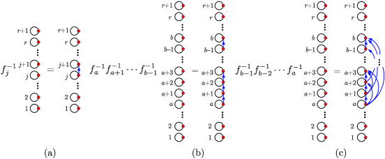
Figure 14: Pictorial representation of the action of (a) $f_{j}^{-1}$, (b) an increasing product $f_{a}^{-1}f_{a+1}^{-1}\cdots f_{b-1}^{-1}$, and (c) a decreasing product $f_{b-1}^{-1}f_{b-2}^{-1}\cdots f_{a}^{-1}$ for some $a<b$. These correspond to adding (a) an ascending edge $j\to j+1$ with weight $-1$, (b) ascending edges $a+i\to a+i+1$, $i=0,1,\dots,b-a-1$ with weights $-1$, and (c) a web of ascending edges $a+i\to a+k$, $0\leq i\leq k-1\leq b-a-1$ with weights $(-1)^{i+k}$.

Recall that the segments $[a_{2i-1},a_{2i}]$ correspond to the ascending segments of ${\mathbf{m}}$, themselves associated to the vertical chain-like pieces of $\Gamma_{\mathbf{m}}$ (see Fig. 8). Recall that in the identification procedure leading to $\Gamma_{\mathbf{m}}^{\prime}$ (Definition 6.7 and Lemma 6.8), we showed that such chains must receive a web of ascending edges with alternating weights $\pm 1$ (see Fig. 11 (c)), while all the vertices are connected via ascending edges $i\to i+1$ with weight $1$.

Finally, comparing this with the graph associated to $(f_{i_{1}}f_{i_{2}}\cdots f_{i_{k}})^{-1}$ as described above, we find that the contribution of ascending edges to $T_{\mathbf{m}}^{\prime}$ (or equivalently, $\Gamma_{\mathbf{m}}^{\prime}$) is identical to $I-(f_{i_{1}}f_{i_{2}}\cdots f_{i_{k}})^{-1}$.

The proof of equation (7.4) is similar, but now concerns the descending edges and the loops of the graph $\Gamma_{{\mathbf{m}}}^{\prime}$.

The product $td_{1}d_{2}\cdots d_{r+1}$ is the transfer matrix of a chain of $r+1$ disconnected vertices $i=1,2,\dots,r+1$, each with a loop with weight $ty_{2i-1}$. Multiplication on the right by $e_{i}$ creates a descending edge $i+1\to i$, with weight $ty_{2i-1}{y_{2i}\over y_{2i-1}}=ty_{2i}$.

Again we divide the sequence $\tau_{\mathbf{m}}$ into increasing subsequences of consecutive integers, $(b_{2j-1}$, $b_{2j-1}+1,\dots,b_{2j})$ and decreasing subsequences $(b_{2j+1}-1,\dots,b_{2j}+1)$. Therefore the product $e_{j_{1}}e_{j_{2}}\cdots e_{j_{r}}$ consists of “ascending” factors

$$Q^{+}_{j}=e_{b_{2j-1}}e_{b_{2j}}\cdots e_{b_{2j}}=I+\sum_{i=1}^{b_{2j}-b_{2j-1}}\sum_{k=0}^{i-1}y_{b_{2j-1}+i,b_{2j-1}+k}E_{b_{2j-1}+k,b_{2j-1}+i}$$

and “descending” factors

$$Q^{-}_{j}=e_{b_{2j+1}-1}e_{b_{2j+1}-2}\cdots e_{b_{2j}+1}=I+\sum_{i=1}^{b_{2j+1}-b_{2j}-1}\frac{y_{2b_{2j}+2i}}{y_{2b_{2j}+2i-1}}\,E_{b_{2j}+i,b_{2j}+i+1},$$

where $y_{b+i,b+j}$ are the weights of equation (6.1).

Recall that the segments $[b_{2i-1},b_{2i}]$ correspond to the descending segments of ${\mathbf{m}}$, which correspond to networks of descending edges on $\Gamma_{\mathbf{m}}$ with weights (6.1) (see Fig. 8). In our construction 6.7 of $\Gamma_{\mathbf{m}}^{\prime}$, these descending edges have remained unchanged, while each vertex $i$ received a loop with weight $ty_{2i-1}$, $i=1,2,\dots,r+1$. This is nothing but the graph associated to $t(d_{1}d_{2}\cdots d_{r+1})(e_{j_{1}}e_{j_{2}}\cdots e_{j_{r}})$, which therefore encodes the contribution of loops and descending edges to $T_{\mathbf{m}}^{\prime}$, and equation (7.4) follows.

We can now make a direct connection with totally positive matrices encoding the networks associated to the Coxeter double Bruhat cells considered in [16]. Each Motzkin path ${\mathbf{m}}\in{\mathcal{M}}_{r}$ corresponds to such an element, the $(r+1)\times(r+1)$ matrix $P_{\mathbf{m}}$:

Definition 7.5.

Given a Motzkin path ${\mathbf{m}}\in\mathcal{M}_{r}$, define

$$P_{{\mathbf{m}}}=(f_{i_{1}}f_{i_{2}}\cdots f_{i_{r}})\,(d_{1}d_{2}\cdots d_{r+1})\,(e_{j_{1}}e_{j_{2}}\cdots e_{j_{r}}),$$

where $(i_{1}i_{2}\cdots i_{r})=\sigma_{\mathbf{m}}$ and $(j_{1}j_{2}\cdots j_{r})=\tau_{\mathbf{m}}$ are the two sequences of (7.2). The parameters $\lambda_{j}$, $\mu_{j}$, $\nu_{j}$ are as in equation (7.5).

As a consequence of equations (7.3), (7.4), we have

Theorem 7.6.

$$(I-T_{\mathbf{m}}^{\prime})^{-1}=(I-tP_{\mathbf{m}})^{-1}\,(f_{i_{1}}f_{i_{2}}\cdots f_{i_{r}}),$$

which allows to rewrite the generating function of Theorem 6.9

$$\big{(}(I-T_{\mathbf{m}}^{\prime})^{-1}\big{)}_{1,1}=\left\{\begin{matrix}\big{(}(I-tP_{\mathbf{m}})^{-1}\big{)}_{1,1}+\big{(}(I-tP_{\mathbf{m}})^{-1}\big{)}_{1,2}&\ \ {\rm if}\ \ a_{1}>1,\vspace{1mm}\\ \displaystyle\sum_{a=a_{1}}^{a_{2}+1}\big{(}(I-tP_{\mathbf{m}})^{-1}\big{)}_{1,a}&\ \ {\rm if}\ \ a_{1}=1.\end{matrix}\right.$$

This yields an interpretation of the solution $R_{1,n+m_{1}+1}$ to the $A_{r}$ $Q$-system with initial data ${\mathbf{x}}_{\mathbf{m}}$ in terms of the network associated to the totally positive matrix $P_{\mathbf{m}}$, for all $n\geq 0$.

Example 7.7.

For the fundamental Motzkin path ${\mathbf{m}}={\mathbf{m}}_{0}$ with $m_{\alpha}=0$ for all ${\alpha}$, we have $\sigma_{{\mathbf{m}}_{0}}=\tau_{{\mathbf{m}}_{0}}=(r,r-1,\dots,1)$, and therefore $P_{{\mathbf{m}}_{0}}=(f_{r}f_{r-1}\cdots f_{1})(d_{1}d_{2}\cdots d_{r+1})(e_{r}e_{r-1}\cdots e_{1})$. Note that the matrix $F=f_{r}f_{r-1}\cdots f_{1}$ has entries $F_{i,j}=1$ if $i\geq j$, and $0$ otherwise. One can check directly that $I-tP_{{\mathbf{m}}_{0}}=F(I-T_{{\mathbf{m}}_{0}}^{\prime})$, with $T_{{\mathbf{m}}_{0}}^{\prime}$ given by equation (4.6).

An equivalent formulation uses the explicit decomposition $P_{\mathbf{m}}=FDE$, where $F=f_{i_{1}}\cdots f_{i_{r}}$, $D=d_{1}\cdots d_{r+1}$ and $E=e_{j_{1}}\cdots e_{j_{r}}$:

$$(I-tP_{\mathbf{m}})^{-1}F=\sum_{n=0}^{\infty}t^{n}(FDE)^{n}F=\sum_{n=0}^{\infty}t^{n}F(DEF)^{n}=F(I-tP_{\mathbf{m}}^{\prime})^{-1},$$

where $P^{\prime}_{\mathbf{m}}=DEF=F^{-1}P_{\mathbf{m}}F$, and the fact that $F$ is a lower uni-triangular matrix, which implies: $\big{(}(I-tT^{\prime}_{\mathbf{m}})^{-1}\big{)}_{1,1}=\big{(}(I-tP_{\mathbf{m}})^{-1}F\big{)}_{1,1}=\big{(}(I-tP^{\prime}_{\mathbf{m}})^{-1}\big{)}_{1,1}$.

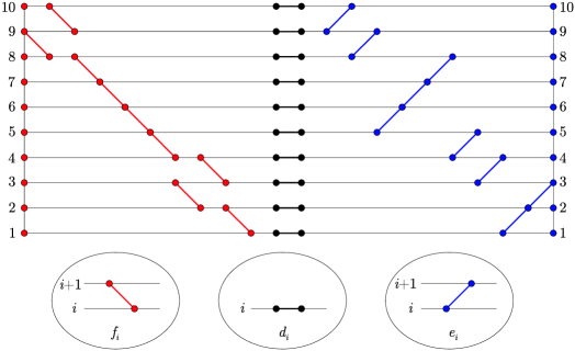
Figure 15: The network corresponding to the totally positive matrix $P_{{\mathbf{m}}}$ for the Motzkin path ${\mathbf{m}}$ of Example 7.2, depicted in Fig. 12 (c). We have indicated in medallions the three network representations (in red, black, blue) for the elementary matrices $f_{i}$, $d_{i}$ and $e_{i}$. The network for $P_{\mathbf{m}}^{\prime}$ corresponds to the same picture, but with the $f$ part (red descending elements) to the right of the $e$ part (ascending blue elements).

The matrix $P^{\prime}_{\mathbf{m}}$ is another way to write a totally positive matrix, and the network graph corresponding to it has a slightly modified form from that of $P_{\mathbf{m}}$. Both of these correspond to electrical networks [14]. For illustration, we represent in Fig. 15 the network corresponding to the matrix $P_{\mathbf{m}}$ for the Motzkin path ${\mathbf{m}}$ of Example 7.2, represented in Fig. 12 (c). The medallions show the three elementary circuit representations for the three types of elementary matrices $f_{i}$, $d_{i}$, $e_{i}$, each receiving the associated weight. The Lindström lemma [24] of network theory states that the minor $|P|_{r_{1},\dots,r_{k}}^{c_{1},\dots,c_{k}}$ of the matrix $P$ of the network, corresponding to a specific choice rows $r_{1},\dots,r_{k}$ and columns $c_{1},\dots,c_{k}$, is the partition function of $k$ non-intersecting (vertex-disjoint) paths starting at points $r_{1},\dots,r_{k}$ and ending at points $c_{1},\dots,c_{k}$, and with steps taken only on horizontal lines or along $f$, $d$ or $e$ type elements. Here we have only considered circuits with entry and exit point $1$, after possibly several iterations of the same network (each receiving the weight $t$), and whose generating function is precisely the resolvent $\big{(}(I-tP)^{-1}\big{)}_{1,1}$.

8 Conclusion

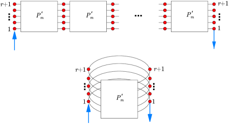
Figure 16: The concatenation of $n$ copies of the network coded by $P_{\mathbf{m}}^{\prime}$. The quantity $(P_{\mathbf{m}}^{\prime})^{n}_{1,1}$ is the partition function of electrical wires starting and ending at the two indicated arrows. We also represent below a cylinder formulation à la [16]: the wire must wind $n$ times around the cylinder before exiting.

In this paper, we have made the contact between our earlier study of the solutions of the $A_{r}$ $Q$-system, expressed in terms of initial data coded via Motzkin paths, and the totally positive matrices for Coxeter double Bruhat cells. We showed in particular how the relevant pairs of Coxeter elements were encoded in the Motzkin paths as well.

One would expect the total positivity of the transfer matrices $P_{\mathbf{m}}$ or $P_{\mathbf{m}}^{\prime}$ to be directly related to the proof of the positivity conjecture in the case of the $A_{r}$ $Q$-system. Our proof presented in [8] relies on the path formulation of $R_{1,n}$ and on the formulation of $R_{{\alpha},n}$ as the partition function of families of strongly non-intersecting paths. The total positivity of the compactified formulation should provide an alternative proof, using networks rather than paths.

The precise connection between paths on graphs and networks, as illustrated in Section 7 above is subtle. Indeed, the identity between resolvents implies that the partition function for weighted paths from $1$ to $1$ on $\Gamma_{\mathbf{m}}$ with $n$ descents, $(T_{\mathbf{m}}^{n})_{1,1}$, is identical to the generating function for circuits on a network made of $n$ identical concatenated networks, each corresponding to the totally positive matrix $P^{\prime}_{\mathbf{m}}$, from connector $1$ to connector $1$ (see the top of Fig. 16). In [16], this concatenation is realized by putting the network on a cylinder and allowing for the circuit to wind $n$ times around it before exiting (see the bottom of Fig. 16). Note that we could also work with $P_{\mathbf{m}}$ instead, as it is related to $P_{\mathbf{m}}^{\prime}$ via cyclic symmetry.

More generally, it should be possible to relate our non-intersecting path families to networks with multiple entries and exits, as in the setting of the Lindström lemma.

Another question concerns the cluster algebra attached to the $A_{r}$ $Q$-system. As stressed in [8], we have only considered a subset of the clusters which arise in the full $Q$-system cluster algebra, namely those which consist of solutions of the $Q$-system. There are other cluster mutations, however, which are not recursion relations of the form (4.1). One may ask about the other cluster variables in the algebra. The positivity conjecture should hold for them as well. Preliminary investigations show that the corresponding mutations can still be understood in terms of (finite) continued fraction rearrangements, hence we expect them to also have a network counterpart. These clearly can no longer correspond to Coxeter double Bruhat cells, as those are exhausted by the solutions of the $Q$-system.

Finally, the connection to total positivity should be generalizable to the case of other simple Lie algebras as well. Indeed, on the one hand the $Q$-systems based on other Lie algebras also have cluster algebra formulations [7], while on the other hand the notion of total positivity has been extended to arbitrary Lie groups [12]. We have evidence that hard particle and path interpretations exist for all $Q$-systems, and it would be interesting to investigate their relation to the corresponding generalized networks. The integrability of these systems is presumably related to that of the Coxeter–Toda systems of [27]. This will be the subject of forthcoming work.

Acknowledgements

We thank M. Gekhtman, S. Fomin, A. Postnikov, N. Reshetikhin and A. Vainshtein for useful discussions. RK’s research is funded in part by NSF grant DMS-0802511. RK thanks CEA/Saclay IPhT for their hospitality. PDF’s research is partly supported by the European network grant ENIGMA and the ANR grants GIMP and GranMa. PDF thanks the department of Mathematics of the University of Illinois at Urbana-Champaign for hospitality and support, and the department of Mathematics of the University of California Berkeley for hospitality.

References

- [1]
- [2] Adler M., van Moerbeke P., Integrals over classical groups, random permutations, Toda and Toeplitz lattices, Comm. Pure Appl. Math. 54 (2001), 153–205, math.CO/9912143.
- [3] Assem I., Reutenauer C., Smith D., Frises, arXiv:0906.2026.
- [4] Berenstein A., Private communication.
-
[5]
Bouttier J., Di Francesco P., Guitter E.,
Geodesic distance in planar graphs,
Nuclear Phys. B 663 (2003), 535–567,
cond-mat/0303272.
Bouttier J., Di Francesco P., Guitter E., Random trees between two walls: exact partition function, J. Phys. A: Math. Gen. 36 (2003), 12349–12366, cond-mat/0306602. - [6] Caldero P., Zelevinsky A., Laurent expansions in cluster algebras via quiver representations, Mosc. Math. J. 6 (2006), 411–429, math.RT/0604054.
- [7] Di Francesco P., Kedem R., -systems as cluster algebras. II. Cartan matrix of finite type and the polynomial property, Lett. Math. Phys. 89 (2009), 183–216, arXiv:0803.0362.
- [8] Di Francesco P., Kedem R., -systems, heaps, paths and cluster positivity, Comm. Math. Phys. 293 (2010), 727–802, arXiv:0811.3027.
- [9] Fomin S., Shapiro M., Thurston D., Cluster algebras and triangulated surfaces. I. Cluster complexes, Acta Math. 201 (2008), 83–146, math.RA/0608367.
- [10] Fomin S., Zelevinsky A., Cluster algebras. I. Foundations, J. Amer. Math. Soc. 15 (2002), 497–529, math.RT/0104151.
- [11] Fomin S., Zelevinsky A., Cluster algebras. IV. Coefficients, Compos. Math. 143 (2007), 112–164, math.RA/0602259.
- [12] Fomin S., Zelevinsky A., Double Bruhat cells and total positivity, J. Amer. Math. Soc. 12 (1999), 335–380, math.RT/9802056.
- [13] Fomin S., Zelevinsky A., The Laurent phenomenon, Adv. in Appl. Math. 28 (2002), 119–144, math.CO/0104241.
- [14] Fomin S., Zelevinsky A., Total positivity: tests and parameterizations, Math. Intelligencer 22 (2000), 23–33, math.RA/9912128.
- [15] Geiss C., Leclerc B., Schröer J., Preprojective algebras and cluster algebras, in Trends in Representation Theory of Algebras and Related Topics, EMS Ser. Congr. Rep., Eur. Math. Soc., Zürich, 2008, 253–283, arXiv:0804.3168.
- [16] Gekhtman M., Shapiro M., Vainshtein A., Generalized Bäcklund–Darboux transformations for Coxeter–Toda flows from cluster algebra perspective, arXiv:0906.1364.
- [17] Gessel I.M., Viennot X., Binomial determinants, paths and hook formulae, Adv. in Math. 58 (1985), 300–321.
- [18] Kazakov V., Kostov I., Nekrasov N., D-particles, matrix integrals and KP hierachy, Nuclear Phys. B 557 (1999), 413–442, hep-th/9810035.
- [19] Kedem R., -systems as cluster algebras, J. Phys. A: Math. Theor. 41 (2008), 194011, 14 pages, arXiv:0712.2695.
- [20] Keller B., Cluster algebras, quiver representations and triangulated categories, arXiv:0807.1960.
- [21] Kirillov A.N., Reshetikhin N.Yu., Representations of Yangians and multiplicity of occurrence of the irreducible components of the tensor product of representations of simple Lie algebras, J. Soviet Math. 52 (1990), 3156–3164.
- [22] Krattenthaler C., The theory of heaps and the Cartier–Foata monoid, Appendix to the electronic republication of Cartier P., Foata D., Problèmes combinatoires de commutation et réarrangements, available at http://www.mat.univie.ac.at/~slc/books/cartfoa.html.
- [23] Krichever I., Lipan O., Wiegmann P., Zabrodin A., Quantum integrable systems and elliptic solutions of classical discrete nonlinear equations, Comm. Math. Phys. 188 (1997), 267–304, hep-th/9604080.
- [24] Lindström B., On the vector representations of induced matroids, Bull. London Math. Soc. 5 (1973), 85–90.
- [25] Musiker G., Schiffler R., Williams L., Positivity for cluster algebras from surfaces, arXiv:0906.0748.
- [26] Propp J., Musiker G., Combinatorial interpretations for rank-two cluster algebras of affine type, Electron. J. Combin. 14 (2007), no. 1, R15, 23 pages, math.CO/0602408.
- [27] Reshetikhin N., Characteristic systems on Poisson Lie groups and their quantization, in Integrable Systems: from Classical to Quantum (Montreal, QC, 1999), CRM Proc. Lecture Notes, Vol. 26, Amer. Math. Soc., Providence, RI, 2000, 165–188, math.CO/0402452.
- [28] Sherman P., Zelevinsky A., Positivity and canonical bases in rank 2 cluster algebras of finite and affine types, Mosc. Math. J. 4 (2004), 947–974, math.RT/0307082.
- [29] Viennot X., Heaps of pieces. I. Basic definitions and combinatorial lemmas, in Combinatoire Énumérative, Editors G. Labelle and P. Leroux, Lecture Notes in Math., Vol. 1234, Springer, Berlin, 1986, 321–350.