Non-Gaussian behaviour of a self-propelled particle on a substrate

Abstract

The overdamped Brownian motion of a self-propelled particle which is driven by a projected internal force is studied by solving the Langevin equation analytically. The “active” particle under study is restricted to move along a linear channel. The direction of its internal force is orientationally diffusing on a unit circle in a plane perpendicular to the substrate. An additional time-dependent torque is acting on the internal force orientation. The model is relevant for active particles like catalytically driven Janus particles and bacteria moving on a substrate. Analytical results for the first four time-dependent displacement moments are presented and analysed for several special situations. For vanishing torque, there is a significant dynamical non-Gaussian behaviour at finite times $t$ as signalled by a non-vanishing normalized kurtosis in the particle displacement which approaches zero for long time with a $1/t$ long-time tail.

I Introduction

The Brownian motion of self-propelled (“active”) particles Ramaswamy ; review_RMP_Haenggi bears much richer physics than the traditional diffusive dynamics of passive particles. Active particles can be modelled by moving under the action of an internal force sometimes combined with an internal or external torque. Realizations in nature are certain bacteria Berg:90 ; DiLuzio:05 ; Lauga:06 ; Hill:07 ; Shenoy:07 and spermatozoa Riedel:05 ; Woolley:03 ; Friedrich which swim in circles when confined to a surface Ohta . In the colloidal world, it is possible to prepare catalytically driven Janus particles Dreyfus:05 ; Dhar:06 ; Walther:08 ; Baraban:08 or biometric particles Fery:08 which perform self-propelled Brownian motion. For a recent investigation including confinement see Popescu:09 . On the macroscopic scale vibrated polar granular rods Kudrolli:07 on a planar substrate and even the trajectories of completely blinded and ear-plugged pedestrians Obata:05 can be considered as rough realizations of self-driven Brownian particles. If the particle is embedded in a liquid (a “swimmer”), as characteristic for colloids, the direction of its driving force is fluctuating, in general, according to orientational Brownian motion Doi_Edwards_book ; HL_Cyl ; Klein . This gives rise to a non-ballistic translational motion of the particles which is coupled to the fluctuating orientational degree of freedom.

In most cases the direction of the self-propelling force is within the plane of motion. For colloidal particles, however, it is possible to confine the particle on a substrate by using, e.g., strong gravity such that the particles are still freely rotating Baraban:08 ; Baraban2 ; Baraban_private though they are confined in a planar monolayer. In this situation the component of the self-propelling force which is normal to the surface is compensated by the substrate, i.e., only the projection of the self-propelling force onto the plane is driving the particle. Therefore the translational motion is coupled to the (Brownian) orientational motion Teeffelen_PRE .

In this paper we consider a one-dimensional model Cates for the Brownian dynamics of a self-propelled particle on a substrate. The particle is self-propelled along its orientational axis, which itself is subjected to Brownian orientational diffusion. The particle is confined to a channel, however, such that only the projected force in channel direction is acting to drive the particle. The present study is more general than earlier work in reference Teeffelen_PRE : first of all, the present calculation resolves the Cartesian components of the isotropic model on an unconfined plane. Second, an arbitrary time-dependence of the external torque is included here while this torque was constant in Teeffelen_PRE . Finally, we calculate time-dependent moments of the particle displacement up to fourth order as compared to results up to second order in reference Teeffelen_PRE . The results are discussed for several special cases. In general, long-time self-diffusion is found. Non-Gaussian behaviour is found for intermediate times as signalled in the corresponding fourth cumulant. The normalized kurtosis is positive for small times, then changes sign and approaches zero from below at long times with a $1/t$ long-time tail. This can be compared to recent investigations for an undriven Brownian ellipsoid Han:06 . In the latter case, the kurtosis was found to be positive approaching zero from above for long times with the same $1/t$ long-time tail.

This work represents a first step towards a many-body situation of interacting self-propelled particles. These are also realizable in experiments (see, e.g., Dreyfus:05 ; Baraban:08 ; Kudrolli:07 ). The suitable theoretical framework is the many-body Smoluchowski equation Dhont_book , from which one can derive a coupled hierarchy of equations for the set of many-body distribution functions similar in spirit to the traditional BBGKY (Bogolyubov-Born-Green-Kirkwood-Yvon) hierarchy Bogolyubov1 ; Bogolyubov2 ; Uhlenbeck for Liouville dynamics, see also Felderhof Felderhof for a discussion in the context of Brownian motion. Therefore we think that this paper is particularly appropriate for this issue dedicated to the 100th anniversary of Prof. N. N. Bogolyubov.

This paper is organized as follows: In section II, we propose and motivate the model. The first four displacement moments are calculated analytically for the torque-free case in section III, while section IV contains the results for a general time-dependent torque. Finally, in section V, we conclude and give an outlook on possible future activities.

II The model

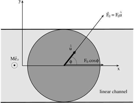
Figure 1: Sketch of the model system: A spherical colloidal particle (dark grey) is confined to a linear channel (light grey) along the $x$-direction. The self-propulsion is modelled by a constant effective force $\vec{F}_{0}$ along the particle orientation $\hat{\vec{u}}$. The latter is constrained to rotate in the $xy$-plane. Only the projected force $F_{0}\cos\phi$ drives the particle along the channel. A systematic, time-dependent torque $\vec{M}(t)=M(t)\hat{\vec{e}}_{z}$ is also indicated.

The model system under study consists of a self-propelled colloidal sphere of radius $R$, which is confined to an infinite linear channel in the $x$-direction, where it undergoes completely overdamped Brownian motion (for a sketch see figure 1). Whereas the motion of the center-of-mass position $x$ is constrained to one dimension, the orientation vector $\hat{\vec{u}}=(\cos\phi,\sin\phi,0)$ is constrained to rotate in the $xy$-plane. The self-propulsion of the particle is modelled by a constant effective force along the particle orientation $\vec{F}=F_{0}\hat{\vec{u}}$ and a generally time-dependent effective torque in the $z$-direction $\vec{M}=M\hat{\vec{e}}_{z}$. Because the particle is confined, only the projected force $\vec{F}\cdot\hat{\vec{e}}_{x}=F_{0}\cos\phi\hat{\vec{e}}_{x}$ drives the particle systematically along the channel. Based on these considerations, the translational and orientational motion is modelled by a Langevin equation for the center-of-mass position $x$ and the orientation vector $\hat{\vec{u}}$:

$$\frac{\mathrm{d}x}{\mathrm{d}t} = \beta D\left[F_{0}\cos\phi+f(t)\right]\,,$$ (1)

$$\frac{\mathrm{d}\hat{\vec{u}}}{\mathrm{d}t} = \beta D_{\mathrm{r}}\left[M(t)+g(t)\right]\hat{\vec{e}}_{z}\times\hat{\vec{u}}\,,$$ (2)

where $f(t)$ is a zero-mean, Gaussian white noise random force, which is characterized by $\langle f(t)\rangle=0$ and $\langle f(t)f(t^{\prime})\rangle=2\delta(t-t^{\prime})/(\beta^{2}D)$, where angular brackets denote a noise average. Correspondingly, $g(t)$ is a Gaussian white noise random torque with $\langle g(t)\rangle=0$ and $\langle g(t)g(t^{\prime})\rangle=2\delta(t-t^{\prime})/(\beta^{2}D_{\mathrm{r}})$. Here, $\beta^{-1}=k_{\mathrm{B}}T$ denotes the thermal energy. $D$ and $D_{\mathrm{r}}$ are the translational and rotational short-time diffusion constants, respectively. For a sphere of radius $R$ in the three-dimensional bulk the two quantities fulfill the relationship

$$\frac{D}{D_{\mathrm{r}}}=\frac{4R^{2}}{3}\,.$$ (3)

Due to the constraint on the orientational motion, the vector equation (2) reduces to a Langevin equation for the orientational angle $\phi$, which is given by

$$\frac{\mathrm{d}\phi}{\mathrm{d}t}=\beta D_{\mathrm{r}}\left[M(t)+g(t)\right]\,.$$ (4)

If the initial time $t_{0}$ is set to be zero, the solutions of the Langevin equations (1) and (4) are given by

$$\phi(t)=\beta D_{\mathrm{r}}\int_{0}^{t}{\left[M(t^{\prime})+g(t^{\prime})\right]\mathrm{d}t^{\prime}}+\phi_{0}$$ (5)

and

$$x(t)=\beta D\left[F_{0}\int_{0}^{t}{\cos\phi(t^{\prime})\mathrm{d}t^{\prime}}+\int_{0}^{t}{f(t^{\prime})\mathrm{d}t^{\prime}}\right]+x_{0}$$ (6)

with $\phi_{0}\equiv\phi(t_{0})$ and $x_{0}\equiv x(t_{0})$.

The translation-rotation-coupling between these two equations, which is due to the cosine in equations (1) and (6), leads to nontrivial results for the mean position $\langle x-x_{0}\rangle$ and the mean square displacement $\langle(x-x_{0})^{2}\rangle$ of the particle position, as is shown in the following sections. Furthermore, the presence of the coupling term leads to non-Gaussian behaviour, which is reflected in a non-zero kurtosis. The latter is obtained by calculating the fourth moment of the particle displacement distribution further down.

We start our analysis in section III by studying the special case of a vanishing systematic torque $M=0$. The more complex situations of a constant torque $M(t)=M$ and a generally time-dependent torque $M(t)$ are considered in section IV.

III Results for a vanishing torque

In this section, the simplest case with a vanishing torque is covered. Solving equation (4) for $M(t)\equiv 0$ and averaging gives

$$\left\langle\phi(t)\right\rangle=\phi_{0}$$ (7)

and for the second moment

$$\left\langle(\phi(t)-\phi_{0})^{2}\right\rangle=2D_{\mathrm{r}}t.$$ (8)

As $\phi(t)$ is a linear combination of Gaussian variables $g(t^{\prime})$, according to Wick’s theorem Doi_Edwards_book , $\phi(t)$ is Gaussian as well. Thus the probability distribution of $\phi$ proves to be

$$P(\phi,t)=\frac{1}{\sqrt{4\pi D_{\mathrm{r}}t}}\exp\left({-\frac{(\phi-\phi_{0})^{2}}{4D_{\mathrm{r}}t}}\right).$$ (9)

Now the mean position of the particle can be calculated. From

$$\langle\cos\phi(t)\rangle=\int_{-\infty}^{\infty}{\cos(\phi)P(\phi,t)\mathrm{d}\phi}=e^{-D_{\mathrm{r}}t}\cos\phi_{0}$$ (10)

follows

$$\langle x(t)-x_{0}\rangle=\frac{4}{3}\beta F_{0}R^{2}\cos(\phi_{0})\left[1-e^{-D_{\mathrm{r}}t}\right],$$ (11)

where we made use of equation (3). Thus for short times one obtains

$$\langle x(t)-x_{0}\rangle=\frac{4}{3}\beta F_{0}R^{2}\cos(\phi_{0})D_{\mathrm{r}}t+\mathcal{O}\left(t^{2}\right)$$ (12)

and for $t\gg D_{\mathrm{r}}^{-1}$ the $\phi_{0}$-dependent mean position converges towards

$$\lim_{t\to\infty}\langle x(t)-x_{0}\rangle=\frac{4}{3}\beta F_{0}R^{2}\cos(\phi_{0}).$$ (13)

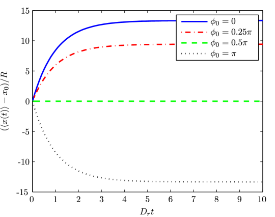
Figure 2: Mean position of a spherical particle without external torque for $\beta RF_{0}=10$ and different values of $\phi_{0}$.

The trajectory of the mean position $\langle x(t)\rangle$ is shown in figure 2 where the time $t$ is given in units of $D_{\mathrm{r}}^{-1}$, while the length $x$ is scaled by the particle radius $R$.

To calculate the mean square displacement, the following integrals have to be solved:

$$\left\langle(x(t)-x_{0})^{2}\right\rangle = \beta^{2}D^{2}\Bigl{[}F_{0}^{2}\int_{0}^{t}\mathrm{d}t_{1}\int_{0}^{t}\mathrm{d}t_{2}\langle\cos\phi(t_{1})\cos\phi(t_{2})\rangle$$ (14)

$$+2F_{0}\int_{0}^{t}\mathrm{d}t_{1}\int_{0}^{t}\mathrm{d}t_{2}\langle\cos\phi(t_{1})f(t_{2})\rangle+\int_{0}^{t}\mathrm{d}t_{1}\int_{0}^{t}\mathrm{d}t_{2}\langle f(t_{1})f(t_{2})\rangle\Bigr{]}.$$

The third summand can be calculated easily and equals $2t/(\beta^{2}D)$. As $\langle\cos\phi(t)\rangle$ only depends on the random torque $g(t)$, $\langle\cos\phi(t)\rangle$ and $f(t)$ are statistically independent. Therefore the second summand vanishes. To calculate the first summand in equation (14), the time correlation function is used. With $\phi_{1}\equiv\phi(t_{1})$ and $\phi_{2}\equiv\phi(t_{2})$ the required average can be written as

$$\left\langle\cos\phi_{1}\cos\phi_{2}\right\rangle_{t_{1}>t_{2}}=\int d\phi_{1}\int d\phi_{2}\cos\phi_{1}\cos\phi_{2}G(\phi_{1},\phi_{2},t_{1}-t_{2})P(\phi_{2},t_{2})|_{t_{1}>t_{2}}.$$ (15)

Here, $G(\phi_{1},\phi_{2},t_{1}-t_{2})$ is the Green function, which is given by

$$G(\phi_{1},\phi_{2},t_{1}-t_{2})=\frac{1}{\sqrt{4\pi D_{\mathrm{r}}(t_{1}-t_{2})}}\exp\left({-\frac{(\phi_{1}-\phi_{2})^{2}}{4D_{\mathrm{r}}(t_{1}-t_{2})}}\right).$$ (16)

This yields

$$\left\langle\cos\phi_{1}\cos\phi_{2}\right\rangle_{t_{1}>t_{2}}=\frac{1}{2}e^{-D_{\mathrm{r}}(t_{1}-t_{2})}\left[1+\cos(2\phi_{0})e^{-4D_{\mathrm{r}}t_{2}}\right].$$ (17)

The expression for $\langle\cos\phi_{1}\cos\phi_{2}\rangle_{t_{2}>t_{1}}$ is obtained in exactly the same way by replacing $t_{1}$ and $t_{2}$ with each other. Now, the first summand in formula (14) is calculated by simple integration and the mean square displacement can be written in the final form

$$\left\langle(x(t)-x_{0})^{2}\right\rangle=2Dt+\left(\frac{4}{3}\beta F_{0}R^{2}\right)^{2}\left[e^{-D_{\mathrm{r}}t}+D_{\mathrm{r}}t-1+\frac{1}{12}\cos(2\phi_{0})\left(e^{-4D_{\mathrm{r}}t}-4e^{-D_{\mathrm{r}}t}+3\right)\right].$$ (18)

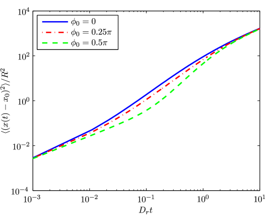
Figure 3: Mean square displacement of a spherical particle for $\beta RF_{0}=10$ and different values of $\phi_{0}$.

The long-time diffusion coefficient $D_{\mathrm{l}}$ is given by

$$D_{\mathrm{l}}=\lim_{t\to\infty}\frac{1}{2t}\left\langle(x(t)-x_{0})^{2}\right\rangle=D+\frac{8}{9}\left(\beta F_{0}R^{2}\right)^{2}D_{\mathrm{r}}.$$ (19)

Figure 3 displays the results for the same cases that were examined in figure 2. The graph for $\phi_{0}=\pi$ coincides with the graph for $\phi_{0}=0$. As can be seen in the logarithmic plots and from the expression (19), the initial angle $\phi_{0}$ is not relevant for times much longer than $D_{\mathrm{r}}^{-1}$.

In the following the non-Gaussian behaviour of the particle is investigated. For this purpose skewness $S$ and kurtosis $\gamma$ are calculated. The non-Gaussian behaviour is clearly signalled in the nonzero value of these quantities. In general, the skewness is given by

$$S=\frac{\left\langle(x-\langle x\rangle)^{3}\right\rangle}{\left\langle(x-\langle x\rangle)^{2}\right\rangle^{3/2}}=\frac{\langle x^{3}\rangle-3\langle x\rangle\langle x^{2}\rangle+2\langle x\rangle^{3}}{(\langle x^{2}\rangle-\langle x\rangle^{2})^{3/2}},$$ (20)

and the kurtosis is calculated as

$$\gamma=\frac{\left\langle(x-\langle x\rangle)^{4}\right\rangle}{\left\langle(x-\langle x\rangle)^{2}\right\rangle^{2}}-3=\frac{\langle x^{4}\rangle-4\langle x\rangle\langle x^{3}\rangle+6\langle x\rangle^{2}\langle x^{2}\rangle-3\langle x\rangle^{4}}{(\langle x^{2}\rangle-\langle x\rangle^{2})^{2}}-3.$$ (21)

For the third and fourth moments of $x$ – in analogy to equation (14) – one has to solve the integrals

$$\left\langle(x(t)-x_{0})^{3}\right\rangle = \beta^{3}D^{3}\int_{0}^{t}\mathrm{d}t_{1}\int_{0}^{t}\mathrm{d}t_{2}\int_{0}^{t}\mathrm{d}t_{3}\Bigl{[}F_{0}^{3}\langle\cos\phi(t_{1})\cos\phi(t_{2})\cos\phi(t_{3})\rangle$$ (22)

$$+3F_{0}\langle\cos\phi(t_{1})\rangle\langle f(t_{2})f(t_{3})\rangle\Bigr{]}$$

and

$$\left\langle(x(t)-x_{0})^{4}\right\rangle = \beta^{4}D^{4}\int_{0}^{t}\mathrm{d}t_{1}\int_{0}^{t}\mathrm{d}t_{2}\int_{0}^{t}\mathrm{d}t_{3}\int_{0}^{t}\mathrm{d}t_{4}\Bigl{[}F_{0}^{4}\langle\cos\phi(t_{1})\cos\phi(t_{2})\cos\phi(t_{3})\cos\phi(t_{4})\rangle$$ (23)

$$+6F_{0}^{2}\langle\cos\phi(t_{1})\cos\phi(t_{2})\rangle\langle f(t_{3})f(t_{4})\rangle+\langle f(t_{1})f(t_{2})f(t_{3})f(t_{4})\rangle\Bigr{]},$$

respectively. Before solving the time-integrals over the first summands, the time correlation functions

$$\left\langle\cos\phi_{1}\cos\phi_{2}\cos\phi_{3}\right\rangle_{t_{1}>t_{2}>t_{3}} \!\!=\!\! \frac{1}{2}\cos(\phi_{0})e^{-D_{\mathrm{r}}(t_{1}-t_{2}+t_{3})}$$ (24)

$$+\frac{1}{4}e^{-D_{\mathrm{r}}(t_{1}+3t_{2}-4t_{3})}\left[\cos(\phi_{0})e^{-D_{\mathrm{r}}t_{3}}+\cos(3\phi_{0})e^{-9D_{\mathrm{r}}t_{3}}\right]\qquad$$

and

$$\left\langle\cos\phi_{1}\cos\phi_{2}\cos\phi_{3}\cos\phi_{4}\right\rangle_{t_{1}>t_{2}>t_{3}>t_{4}}$$ (25)

$$= \frac{1}{4}e^{-D_{\mathrm{r}}(t_{1}-t_{2}+t_{3}-t_{4})}\left[1+\cos(2\phi_{0})e^{-4D_{\mathrm{r}}t_{4}}\right]$$

$$+\frac{1}{4}e^{-D_{\mathrm{r}}(t_{1}+3t_{2}-4t_{3})}\Bigl{\{}\frac{1}{2}e^{-D_{\mathrm{r}}(t_{3}-t_{4})}\left[1+\cos(2\phi_{0})e^{-4D_{\mathrm{r}}t_{4}}\right]$$

$$+\frac{1}{2}e^{-9D_{\mathrm{r}}(t_{3}-t_{4})}\left[\cos(4\phi_{0})e^{-16D_{\mathrm{r}}t_{4}}+\cos(2\phi_{0})e^{-4D_{\mathrm{r}}t_{4}}\right]\Bigr{\}}\qquad$$

have to be evaluated. Here the notation $\phi_{i}\equiv\phi(t_{i})$ with $i\in\{1,2,3,4\}$ is used again. Both in equation (22) and in equation (23), the remaining terms can be calculated easily using the expressions already obtained for the first and second moments. The complete analytical results for the third and fourth moments (and for the skewness and kurtosis) are presented in the appendix.

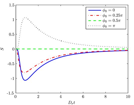
Figure 4: Skewness $S(t)$ for $\beta RF_{0}=10$ and different values of $\phi_{0}$.

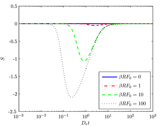
Figure 5: Skewness $S(t)$ for $\phi_{0}=0$ and different values of $\beta RF_{0}$.

Figures 4 and 5 display the skewness $S$ of the probability distribution of the particle position for different values of the initial angle $\phi_{0}$ and the dimensionless quantity $\beta RF_{0}$ which determines whether the self-propulsion or the motion due to the interaction with the solvent molecules is dominant. Figure 4 shows that the sign of the skewness depends on $\phi_{0}$. If the $x$-component of the initial orientation is positive ($-0.5\pi<\phi_{0}<0.5\pi$), the skewness is negative, while initial angles between $0.5\pi$ and $1.5\pi$ lead to positive $S$. For symmetry reasons the skewness is zero for $\phi_{0}=0.5\pi$. Further analysis of formula (42) (see the appendix) gives the leading long-time behaviour of the skewness $S(t)$ as

$$S(t)=\frac{8}{3}\,{\frac{{a}^{3}\cos\left(\phi_{0}\right)\left(\left(\cos\left(\phi_{0}\right)\right)^{2}-3\right)}{\left(3+2\,{a}^{2}\right)\sqrt{4\,{a}^{2}+6}}}\,{(D_{\mathrm{r}}t)}^{-3/2}+\mathrm{o}\left(\frac{1}{t^{3/2}}\right),$$ (26)

where the abbreviation $a\equiv\beta RF_{0}$ is used, i.e., the skewness decreases proportionally to $t^{-3/2}$.

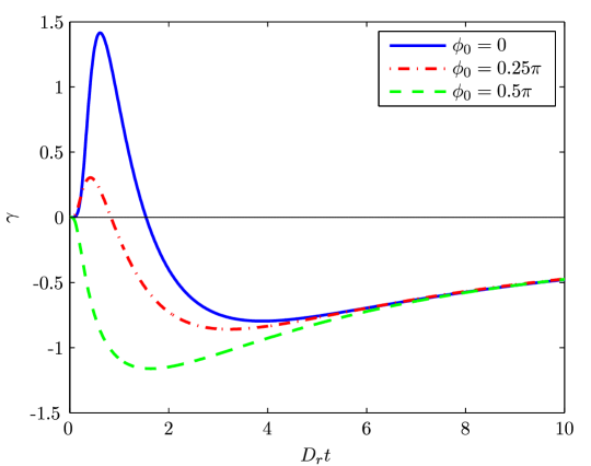
Figure 6: Kurtosis $\gamma(t)$ for $\beta RF_{0}=10$ and different values of $\phi_{0}$.

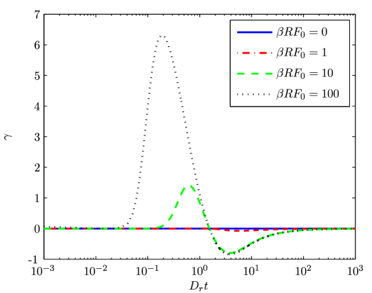
Figure 7: Kurtosis $\gamma(t)$ for $\phi_{0}=0$ and different values of $\beta RF_{0}$.

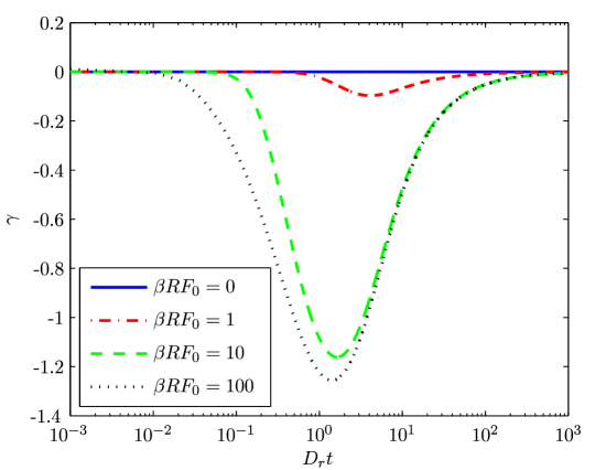
Figure 8: Kurtosis $\gamma(t)$ for $\phi_{0}=0.5\pi$ and different values of $\beta RF_{0}$.

Similar analysis of formula (43) for the kurtosis $\gamma(t)$ reveals a long time behaviour as

$$\gamma(t)={\frac{-21{a}^{4}}{9+12\,{a}^{2}+4\,{a}^{4}}}\,(D_{\mathrm{r}}t)^{-1}+\mathrm{o}\left(\frac{1}{t}\right).$$ (27)

First of all, as can be seen from this formula and in figures 6–8, the kurtosis does not depend on $\phi_{0}$ for long times. The long-time tail, being proportional to $1/t$, is more pronounced than that for the skewness. Moreover, as displayed in figures 6 and 8, for initial angles $\phi_{0}\neq 0.5\pi$ the distribution is leptokurtic (positive kurtosis) for relatively short times and platykurtic (negative kurtosis) for relatively long times. Thus for intermediate times a change of sign is induced such that the kurtosis approaches its asymptotic value zero from below. This is in contrast to passive ellipsoidal particles in two dimensions Han:06 where non-Gaussian behaviour is due to dissipatively coupled translational and rotational motion. In the latter case, the same scaling of the long-time tail proportional to $1/t$ is found for the kurtosis but it approaches zero from above.

We expect that the different sign is linked to the one-dimensionality of our model rather than to the qualitatively different translation-rotation coupling, which is due to the driving force in our model as opposed to the different transverse and parallel short-time translational diffusivities in the passive ellipsoidal particle model. In particular, we expect the negative kurtosis at long times $t\gg D_{r}^{-1}$ to reflect a broad translational van Hove function hansen-mcdonald:86 with shorter tails as compared to a Gaussian distribution, which is attributed to the non-linear $\cos$-term in equation (1).

IV Results for a time-dependent torque

Let us now assume an additional internal or external torque. Before considering the case of an arbitrarily time-dependent torque $M(t)$, we first consider a constant torque $M$. Solving the Langevin equations (1) and (4) under this assumption, one obtains

$$\langle\phi(t)\rangle=\phi_{0}+\beta D_{\mathrm{r}}Mt=\phi_{0}+\omega t$$ (28)

with the frequency $\omega=\beta D_{\mathrm{r}}M$ and

$$\left\langle(\phi(t)-\langle\phi(t)\rangle)^{2}\right\rangle=2D_{\mathrm{r}}t.$$ (29)

By replacing $\phi_{0}$ in formula (9) with $\phi_{0}+\omega t$, the updated probability distribution of $\phi$ is gained. The mean position is obtained as

$$\langle x(t)-x_{0}\rangle = \frac{\beta D}{(D_{\mathrm{r}}^{2}+\omega^{2})}F_{0}\bigl{[}D_{\mathrm{r}}\cos(\phi_{0})-\omega\sin(\phi_{0})$$ (30)

$$+e^{-D_{\mathrm{r}}t}(\omega\sin(\phi_{0}+\omega t)-D_{\mathrm{r}}\cos(\phi_{0}+\omega t))\bigr{]}.$$

In figure 9 this result is plotted for different values of the dimensionless quantity $\beta M$, which is the ratio of the external torque over the thermal energy. The long-time mean position is given by

$$\lim_{t\to\infty}\langle x(t)-x_{0}\rangle=\frac{\beta D}{(D_{\mathrm{r}}^{2}+\omega^{2})}F_{0}\left[D_{\mathrm{r}}\cos(\phi_{0})-\omega\sin(\phi_{0})\right],$$ (31)

while the behaviour for short times is the same as in formula (12) for a vanishing torque.

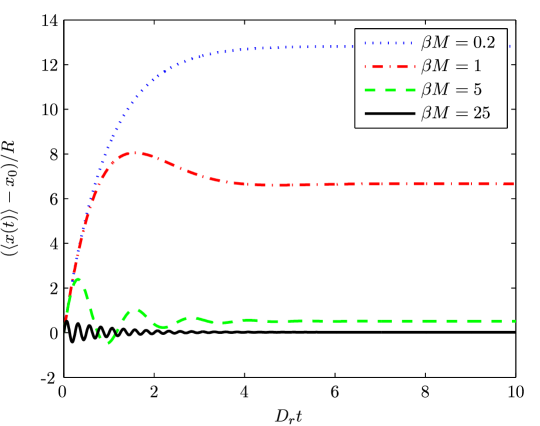
Figure 9: Mean position of a spherical particle with additional constant external torque for $\beta RF_{0}=10$, $\phi_{0}=0$ and different values of $\beta M$.

Following the notation introduced in formula (15) the Green function is now given by

$$G(\phi_{1},\phi_{2},t_{1}-t_{2})=\frac{1}{\sqrt{4\pi D_{\mathrm{r}}(t_{1}-t_{2})}}\exp\left({-\frac{(\phi_{1}-\phi_{2}-\omega(t_{1}-t_{2}))^{2}}{4D_{\mathrm{r}}(t_{1}-t_{2})}}\right).$$ (32)

This leads to

$$\left\langle\cos\phi_{1}\cos\phi_{2}\right\rangle_{t_{1}>t_{2}}=\frac{1}{2}e^{-D_{\mathrm{r}}(t_{1}-t_{2})}\left[\cos(\omega(t_{1}-t_{2}))+\cos\left(2\phi_{0}+\omega(t_{1}+t_{2})\right)e^{-4D_{\mathrm{r}}t_{2}}\right]$$ (33)

and by integration one obtains

$$\left\langle(x(t)-x_{0})^{2}\right\rangle\!\!\! \!=\!\!\! 2Dt+\beta^{2}F_{0}^{2}D^{2}\biggl{\{}\frac{D_{\mathrm{r}}t}{D_{\mathrm{r}}^{2}+\omega^{2}}-\frac{D_{\mathrm{r}}^{2}-\omega^{2}}{(D_{\mathrm{r}}^{2}+\omega^{2})^{2}}$$ (34)

$$-\frac{e^{-D_{\mathrm{r}}t}}{(D_{\mathrm{r}}^{2}+\omega^{2})^{2}}\Bigl{[}(\omega^{2}-D_{\mathrm{r}}^{2})\cos(\omega t)+2\omega D_{\mathrm{r}}\sin(\omega t)\Bigr{]}$$

$$+\frac{1}{(9D_{\mathrm{r}}^{2}+\omega^{2})(D_{\mathrm{r}}^{2}+\omega^{2})}\Bigl{[}e^{-D_{\mathrm{r}}t}\bigl{(}(-3D_{\mathrm{r}}^{2}+\omega^{2})\cos(2\phi_{0}+\omega t)$$

$$+4D_{\mathrm{r}}\omega\sin(2\phi_{0}+\omega)\bigr{)}-(-3D_{\mathrm{r}}^{2}+\omega^{2})\cos(2\phi_{0})-4D_{\mathrm{r}}\omega\sin(2\phi_{0})\Bigr{]}$$

$$+\frac{1}{(9D_{\mathrm{r}}^{2}+\omega^{2})(16D_{\mathrm{r}}^{2}+4\omega^{2})}\Bigl{[}e^{-4D_{\mathrm{r}}t}\bigl{(}(12D_{\mathrm{r}}^{2}-2\omega^{2})\cos(2\phi_{0}+2\omega t)$$

$$-10D_{\mathrm{r}}\omega\sin(2\phi_{0}+2\omega t)\bigr{)}-(12D_{\mathrm{r}}^{2}-2\omega^{2})\cos(2\phi_{0})+10D_{\mathrm{r}}\omega\sin(2\phi_{0})\Bigr{]}\!\!\biggr{\}}.$$

The result is displayed in figure 10. In this case, the long-time diffusion coefficient is given by

$$D_{\mathrm{l}}=D+\frac{8}{9}\frac{(\beta F_{0}R^{2})^{2}D_{\mathrm{r}}}{(1+(\beta M)^{2})}.$$ (35)

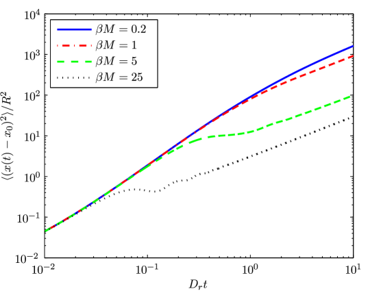
Figure 10: Mean square displacement of a spherical particle with additional constant external torque for $\beta RF_{0}=10$, $\phi_{0}=0$ and different values of $\beta M$.

To generalize the preceding considerations, the torque $M(t)$ is assumed to be arbitrarily time-dependent now. Similarly to the two special cases investigated so far, it can be seen that the mean position of the particle is given by

$$\langle x(t)\rangle=\beta F_{0}D\int_{0}^{t}\cos\left[\phi_{0}+\beta D_{\mathrm{r}}\int_{0}^{t_{1}}M(t_{2})\mathrm{d}t_{2}\right]e^{-D_{\mathrm{r}}t_{1}}\mathrm{d}t_{1}+x_{0}.$$ (36)

The calculation of the mean square displacement starts with formula (14) again. The first summand is the most interesting one because the other ones can be treated as before. Based on the formula

$$\left\langle\cos\phi_{1}\cos\phi_{2}\right\rangle_{t_{1}>t_{2}} = \frac{1}{2}e^{-D_{\mathrm{r}}(t_{1}-t_{2})}\Bigl{[}\cos\left(\beta D_{\mathrm{r}}\int_{t_{2}}^{t_{1}}M(t)\mathrm{d}t\right)$$ (37)

$$+\cos\left(2\phi_{0}+2\beta D_{\mathrm{r}}\int_{0}^{t_{2}}M(t)\mathrm{d}t+\beta D_{\mathrm{r}}\int_{t_{2}}^{t_{1}}M(t)\mathrm{d}t\right)e^{-4D_{\mathrm{r}}t_{2}}\Bigr{]}$$

we introduce

$$\omega_{t_{1}}\! \!:=\! \!\beta D_{\mathrm{r}}\int_{0}^{t_{1}}M(t)\mathrm{d}t,$$

$$\omega_{t_{2}}\! \!:=\! \!\beta D_{\mathrm{r}}\int_{0}^{t_{2}}M(t)\mathrm{d}t.$$ (38)

Using this notation the problem can be solved in a similar way as for a constant $M$. The mean square displacement is now given by

$$\left\langle(x(t)-x_{0})^{2}\right\rangle = 2Dt+\beta^{2}F_{0}^{2}D^{2}\int_{0}^{t}\mathrm{d}t_{1}\int_{0}^{t_{1}}\mathrm{d}t_{2}e^{-D_{\mathrm{r}}(t_{1}-t_{2})}$$ (39)

$$\times\left[\cos(\omega_{t_{1}}-\omega_{t_{2}})+\cos\left(2\phi_{0}+\omega_{t_{1}}+\omega_{t_{2}}\right)e^{-4D_{\mathrm{r}}t_{2}}\right].$$

V Conclusions

In conclusion, motivated by recent experiments on catalytic colloidal particles Baraban:08 ; Baraban2 ; Baraban_private , we have proposed and solved a model for a self-propelled colloidal particle on a substrate. An internal or external time-dependent torque is also included in the most general version of the model which can arise, e.g., from an external magnetic field. The first four moments of the particle displacement distribution were calculated analytically. Significant non-Gaussian behaviour was found for intermediate time. The normalized kurtosis changes sign and approaches zero from below with a massive long-time tail inversely proportional to time.

Future work should address several generalizations of the model. First of all, the one-dimensionality of our model can be generalized towards higher dimensions both for the translational and orientational degrees of freedom. In particular, the translational degrees of freedom can be considered to be two-dimensional (in a plane), and the orientational ones on a sphere. For the latter case, first analytical results have been obtained tenHagen . Also, e.g., for weak gravity, the third translational dimension perpendicular to the substrate is getting important, which results in unusual sedimentation effects Poon . Furthermore, the self-propelled particle can be confined in the lateral direction Baraban_private which leads to a finite mean square displacement. This effect should be incorporated into a model study as well. First results have been obtained for a circle-swimmer in planar circular geometry Zimmermann and for swimmers in cuspy environments leading to self-rotating objects Leonardo .

Last not least, the collective behaviour of many interacting self-propelled particles is expected to lead to novel characteristic nonequilibrium effects both without Viczek:PRL ; EPL_Raina ; Markus_Baer ; Romanczuk:09 and with confinement Leonardo ; Wensink . As stated in the introduction, the Smoluchowski equation, suitably generalized to self-propelled particles Wensink , is an appropriate starting point here and the general hierarchy of Bogolyubov-Born-Green-Kirkwood-Yvon Bogolyubov1 ; Bogolyubov2 ; Uhlenbeck is expected to be a valuable tool in order to derive approximations in a systematic way. This fact after all clearly links the present paper to the 100th anniversary of N. N. Bogolyubov.

Appendix

Using the notation $a=\beta RF_{0}$ and a scaled time $\tau=D_{\mathrm{r}}t$, we summarize here the analytical results for the third and fourth moments as well as for the skewness $S$ and kurtosis $\gamma$:

$$\left\langle\frac{(x(t)-x_{0})^{3}}{R^{3}}\right\rangle = {\frac{32}{3}}\,a\tau\cos\left(\phi_{0}\right)\left(1-{e^{-\tau}}\right)$$ (40)

$$+{\frac{64}{27}}\,{a}^{3}\Bigl{(}-{\frac{45}{8}}\,\cos\left(\phi_{0}\right)+\frac{1}{24}\,\cos\left(3\,\phi_{0}\right)+{\frac{17}{3}}\,\cos\left(\phi_{0}\right){e^{-\tau}}$$

$$-\frac{1}{16}\,\cos\left(3\,\phi_{0}\right){e^{-\tau}}+3\,\cos\left(\phi_{0}\right)\tau-\frac{1}{24}\,\cos\left(\phi_{0}\right){e^{-4\,\tau}}$$

$$+\frac{1}{40}\,\cos\left(3\,\phi_{0}\right){e^{-4\,\tau}}+\frac{5}{2}\,\cos\left(\phi_{0}\right)\tau{e^{-\tau}}-{\frac{1}{240}}\,{e^{-9\,\tau}}\cos\left(3\,\phi_{0}\right)\Bigr{)},\qquad$$

$$\left\langle\frac{(x(t)-x_{0})^{4}}{R^{4}}\right\rangle = {\frac{64}{3}}\,{\tau}^{2}+{\frac{256}{9}}\,{a}^{2}\tau\left({e^{-\tau}}+\tau-1+\frac{1}{12}\,\cos\left(2\,b\right)\left({e^{-4\,\tau}}-4\,{e^{-\tau}}+3\right)\right)$$ (41)

$$+{\frac{256}{81}}\,{a}^{4}\biggl{(}3\,{\tau}^{2}+{\frac{1}{6720}}\,{e^{-16\,\tau}}\cos\left(4\,\phi_{0}\right)-5\,\tau{e^{-\tau}}-{\frac{45}{4}}\,\tau$$

$$+{\frac{261}{16}}+{\frac{1}{600}}\,\cos\left(2\,\phi_{0}\right){e^{-9\,\tau}}-{\frac{19}{6}}\,\cos\left(2\,\phi_{0}\right)+{\frac{1}{240}}\,\cos\left(4\,\phi_{0}\right){e^{-4\,\tau}}$$

$$+{\frac{1}{192}}\,\cos\left(4\,\phi_{0}\right)+\frac{1}{48}\,{e^{-4\,\tau}}-{\frac{49}{3}}\,{e^{-\tau}}-{\frac{7}{450}}\,\cos\left(2\,\phi_{0}\right){e^{-4\,\tau}}$$

$$-{\frac{1}{120}}\,\cos\left(4\,\phi_{0}\right){e^{-\tau}}+\frac{3}{2}\,\tau\cos\left(2\,\phi_{0}\right)-\frac{1}{30}\,\tau\cos\left(2\,\phi_{0}\right){e^{-4\,\tau}}$$

$$+{\frac{229}{72}}\,\cos\left(2\,\phi_{0}\right){e^{-\tau}}-{\frac{1}{840}}\,\cos\left(4\,\phi_{0}\right){e^{-9\,\tau}}+\frac{5}{3}\,\tau\cos\left(2\,\phi_{0}\right){e^{-\tau}}\biggr{)},\qquad$$

$$S = \biggl{[}\frac{8}{3}\,\tau+{\frac{16}{9}}\,{a}^{2}\left({e^{-\tau}}+\tau-1+\frac{1}{12}\,\cos\left(2\,\phi_{0}\right)\left({e^{-4\,\tau}}-4\,{e^{-\tau}}+3\right)\right)$$ (42)

$$-{\frac{16}{9}}\,{a}^{2}\left(\cos\left(\phi_{0}\right)\right)^{2}\left(1-{e^{-\tau}}\right)^{2}\biggr{]}^{-3/2}$$

$$\times\Biggl{\{}-{\frac{32}{9}}\,{a}^{3}\cos\left(\phi_{0}\right)-{\frac{760}{81}}\,{a}^{3}\cos\left(\phi_{0}\right){e^{-\tau}}-{\frac{44}{27}}\,{a}^{3}\cos\left(3\,\phi_{0}\right){e^{-\tau}}-{\frac{32}{81}}\,{a}^{3}\cos\left(\phi_{0}\right){e^{-4\,\tau}}$$

$$-{\frac{32}{135}}\,{a}^{3}\cos\left(3\,\phi_{0}\right){e^{-4\,\tau}}-{\frac{4}{405}}\,{a}^{3}{e^{-9\,\tau}}\cos\left(3\,\phi_{0}\right)+{\frac{32}{81}}\,{a}^{3}\cos\left(3\,\phi_{0}\right)+{\frac{352}{27}}\,{a}^{3}\cos\left(\phi_{0}\right)\tau{e^{-\tau}}$$

$$+{\frac{448}{27}}\,{a}^{3}\cos\left(\phi_{0}\right){e^{-2\,\tau}}+{\frac{64}{27}}\,{a}^{3}{e^{-2\,\tau}}\cos\left(3\,\phi_{0}\right)-{\frac{32}{27}}\,{a}^{3}{e^{-3\,\tau}}\cos\left(3\,\phi_{0}\right)-{\frac{32}{9}}\,{a}^{3}{e^{-3\,\tau}}\cos\left(\phi_{0}\right)$$

$$+{\frac{8}{27}}\,{a}^{3}{e^{-5\,\tau}}\cos\left(\phi_{0}\right)+{\frac{8}{27}}\,{a}^{3}{e^{-5\,\tau}}\cos\left(3\,\phi_{0}\right)\Biggr{\}}$$

and

$$\gamma = \biggl{[}\frac{8}{3}\,\tau+{\frac{16}{9}}\,{a}^{2}\left({e^{-\tau}}+\tau-1+\frac{1}{12}\,\cos\left(2\,\phi_{0}\right)\left({e^{-4\,\tau}}-4\,{e^{-\tau}}+3\right)\right)$$ (43)

$$-{\frac{16}{9}}\,{a}^{2}\left(\cos\left(\phi_{0}\right)\right)^{2}\left(1-{e^{-\tau}}\right)^{2}\biggr{]}^{-2}$$

$$\times\Biggl{\{}-{\frac{128}{9}}\,\tau{a}^{2}{e^{-2\,\tau}}\cos(2\,\phi_{0})+{\frac{64}{81}}\,{a}^{4}{e^{-6\,\tau}}\cos(2\,\phi_{0})+{\frac{64}{3}}\,{\tau}^{2}-{\frac{15424}{729}}\,{a}^{4}{e^{-\tau}}\cos(2\,\phi_{0})$$

$$+{\frac{32}{81}}\,{a}^{4}{e^{-6\,\tau}}\cos(4\,\phi_{0})+{\frac{64}{45}}\,{a}^{4}{e^{-\tau}}\cos(4\,\phi_{0})+{\frac{2032}{27}}\,{a}^{4}-{\frac{128}{3}}\,{a}^{2}\tau$$

$$+{\frac{256}{9}}\,{a}^{2}{\tau}^{2}-{\frac{1216}{27}}\,{a}^{4}\tau+{\frac{256}{27}}\,{a}^{4}{\tau}^{2}+{\frac{64}{27}}\,\tau{a}^{2}{e^{-4\,\tau}}\cos(2\,\phi_{0})-{\frac{70976}{18225}}\,{a}^{4}{e^{-4\,\tau}}\cos(2\,\phi_{0})$$

$$-{\frac{20480}{243}}\,{a}^{4}{e^{-\tau}}-{\frac{688}{243}}\,{a}^{4}{e^{-4\,\tau}}-{\frac{2560}{81}}\,{a}^{4}\tau{e^{-\tau}}+{\frac{512}{9}}\,\tau{a}^{2}{e^{-\tau}}-{\frac{128}{9}}\,\tau{a}^{2}{e^{-2\,\tau}}$$

$$+{\frac{2048}{81}}\,{a}^{4}\tau{e^{-2\,\tau}}-{\frac{1136}{1215}}\,{a}^{4}{e^{-4\,\tau}}\cos(4\,\phi_{0})-{\frac{256}{81}}\,{a}^{4}{e^{-2\,\tau}}\cos(4\,\phi_{0})+{\frac{32}{81}}\,{a}^{4}{e^{-6\,\tau}}$$

$$-{\frac{2560}{243}}\,{a}^{4}\tau{e^{-\tau}}\cos(2\,\phi_{0})+{\frac{4}{8505}}\,{a}^{4}{e^{-16\,\tau}}\cos(4\,\phi_{0})-{\frac{256}{243}}\,{a}^{4}{e^{-5\,\tau}}-{\frac{2048}{1215}}\,{a}^{4}{e^{-5\,\tau}}\cos(2\,\phi_{0})$$

$$+{\frac{2048}{81}}\,{a}^{4}\tau{e^{-2\,\tau}}\cos(2\,\phi_{0})+{\frac{1792}{81}}\,{a}^{4}{e^{-3\,\tau}}+{\frac{1088}{81}}\,{a}^{4}\cos(2\,\phi_{0})-{\frac{20}{81}}\,{a}^{4}\cos(4\,\phi_{0})$$

$$+{\frac{2048}{81}}\,{a}^{4}{e^{-3\,\tau}}\cos(2\,\phi_{0})+{\frac{256}{81}}\,{a}^{4}{e^{-3\,\tau}}\cos(4\,\phi_{0})-{\frac{128}{27}}\,{a}^{4}\tau\cos(2\,\phi_{0})-{\frac{64}{9}}\,{a}^{2}\tau\cos(2\,\phi_{0})$$

$$-{\frac{2336}{243}}\,{a}^{4}{e^{-2\,\tau}}-{\frac{32}{1215}}\,{a}^{4}{e^{-10\,\tau}}\cos(2\,\phi_{0})-{\frac{32}{1215}}\,{a}^{4}{e^{-10\,\tau}}\cos(4\,\phi_{0})-{\frac{3104}{243}}\,{a}^{4}{e^{-2\,\tau}}\cos(2\,\phi_{0})$$

$$+{\frac{64}{2025}}\,{a}^{4}{e^{-9\,\tau}}\cos(2\,\phi_{0})-{\frac{256}{405}}\,{a}^{4}{e^{-5\,\tau}}\cos(4\,\phi_{0})+{\frac{512}{27}}\,{a}^{2}\tau{e^{-\tau}}\cos(2\,\phi_{0})$$

$$-{\frac{128}{1215}}\,{a}^{4}\tau{e^{-4\,\tau}}\cos(2\,\phi_{0})+{\frac{64}{2835}}\,{a}^{4}{e^{-9\,\tau}}\cos(4\,\phi_{0})\Biggr{\}}-3.$$

References

- (1) Toner J., Tu Y., Ramaswamy S., Annals of Physics, 2005, 318, 170.
- (2) Hänggi P., Marchesoni F., Rev. Mod. Phys., 2009, 81, 387.
- (3) Berg H.C., Turner L., Biophys. J., 1990, 58, 919.
- (4) DiLuzio W.R. et al., Nature, 2005, 435, 1271.
- (5) Lauga E., DiLuzio W.R., Whitesides G.M., Stone H.A., Biophys. J., 2006, 90, 400.
- (6) Hill J., Kalkanci O., McMurry J.L., Koser H., Phys. Rev. Lett., 2007, 98, 068101.
- (7) Shenoy V.B., Tambe D.T., Prasad A., Theriot J.A., PNAS, 2007, 104, 8229.
- (8) Riedel I.H., Kruse K., Howard J., Science, 2005, 309, 300.
- (9) Woolley D.M., Reproduction, 2003, 126, 259.
- (10) Friedrich B.M., Jülicher F., New J. Phys., 2008, 10, 123025.
- (11) For a spontaneous rotation of a swimmer, see: Ohta T., Ohkuma T., Phys. Rev. Lett., 2009, 102, 154101.
- (12) Dreyfus R. et al., Nature, 2005, 437, 862.
- (13) Dhar P. et al., Nano Lett., 2006, 6, 66.
- (14) Walther A., Müller A.H.E., Soft Matter, 2008, 4, 663.
- (15) Erbe A. et al., J. Phys.: Condens. Matter, 2008, 20, 404215.
- (16) Schmidt S. et al., Eur. Biophys. J., 2008, 37, 1361.
- (17) Popescu M.N., Dietrich S., Oshanin G., J. Chem. Phys., 2009, 130, 194702.
- (18) Kudrolli A., Lumay G., Volfson D., Tsimring L.S., Phys. Rev. Lett., 2008, 100, 058001.
- (19) Obata T. et al., J. Korean Phys. Soc., 2005, 46, 713.
- (20) Doi M., Edwards S.F., The Theory of Polymer Dynamics, Oxford Science Publications, Oxford, 1986.
- (21) Löwen H., Phys. Rev. E, 1994, 50, 1232.
- (22) Kirchhoff T., Löwen H., Klein R., Phys. Rev. E, 1996, 53, 5011.
- (23) Baraban L. et al., Colloidal Micromotors: Controlled Directed Motion, arXiv:0807.1619v1
- (24) Baraban L., private communication.
- (25) van Teeffelen S., Löwen H., Phys. Rev. E, 2008, 78, 020101(R).
- (26) One-dimensional models for run-and-tumble bacteria have recently been discussed in: Tailleur J., Cates M.E., Phys. Rev. Lett., 2008, 100, 218103.
- (27) Han Y. et al., Science, 2006, 314, 626.
- (28) Dhont J.K.G., An Introduction to Dynamics of Colloids, Elsevier, Amsterdam, 1996.
- (29) Bogolyubov N.N., “Kinetic Equations”, Journal of Physics USSR, 1946, 10, 265.
- (30) Bogolyubov N.N., “Problems of a dynamical theory in statistical physics” (Moscow: Nauka) in Russian, 1946.
- (31) Reference Bogolyubov2 is translated in: de Boer J., Uhlenbeck G.E. (eds.), Studies in Statistical Mechanics, Vol. 1, (Amsterdam, North Holland), 1962.
- (32) Felderhof B.U., J. Phys. A: Math. Gen., 1978, 11, 929.
- (33) Hansen J.-P., McDonald I.R., Theory of simple liquids, Academic Press, London, 2006.
- (34) ten Hagen B., unpublished.
- (35) Barrett-Freeman C., Evans M.R., Marenduzzo D., Poon W.C.K., Phys. Rev. Lett., 2008, 101, 100602.
- (36) Zimmermann U., van Teeffelen S., Löwen H., unpublished.
- (37) Angelani L., Di Leonardo R., Ruocco G., Phys. Rev. Lett., 2009, 102, 048104.
- (38) Vicsek T. et al., Phys. Rev. Lett., 1995, 75, 1226.
- (39) Kirchhoff R., Löwen H., Europhysics Letters, 2005, 69, 291.
- (40) Peruani F., Deutsch A., Bär M., Phys. Rev. E, 2006, 74, 030904(R).
- (41) Romanczuk P., Couzin I.D., Schimansky-Geier L., Phys. Rev. Lett., 2009, 102, 010602.
- (42) Wensink H.H., Löwen H., Phys. Rev. E, 2008, 78, 031409.