Bell inequality tests of Four-Photon Six-Qubit Graph States

Abstract

We demonstrate experimentally a Y-shape graph state with photons’ polarization and spatial modes as qubits for the first time. Based on the state and a linear-type graph state, we report on the experimental realization of two different Bell inequality tests, which represent higher violation than previous Bell tests.

I I. Introduction

Graph states are basic resources for one-way quantum computation RB01 , quantum error-correction SW02 , and studying multiparticle entanglement HEB04 . Moreover, they provide a test-bed to investigate quantum nonlocality, that is, the inconsistency between local hidden variable (LHV) theories and quantum mechanics GTHB05 ; otfried ; avn ; CGR08 ; mermin . Considerable efforts have been devoted to designing different Bell inequalities for graph states with many particles. Here, the aim is to find inequalities with a high quantum mechanical violation, as this is related to the detection efficiency required to perform a loophole-free testing of Bell inequality; moreover, the Bell inequality with a higher violation is more robust against noise. In these studies it has turned out that for many kinds of graph states, the violation of local realism increases exponentially with the number of particles mermin ; otfried . Experimental Bell tests with four-qubit cluster or Greenberger-Horne-Zeilinger (GHZ) states, which are examples of graph states, have been reported recently walther ; Kiesel ; Matini1 ; Zhi .

In this paper we report an experimental realization of a Y-shape graph states Y₆, which are produced using the polarization and the spatial modes of four photons. Such states are also called hyper-entangled states and can be generated with good quality and a high generation rate Kwiat1 ; Kwiat2 ; Matini1 ; Matini2 ; Kai ; bangzi ; Gao . Based on the state and a linear-type one LC₆, we demonstrate two six-qubit Bell tests, which remarkably represent higher violation than previous experiments on Bell tests. In addition, we give a simple theoretical proof that they give the same high violation of local realism as the six-qubit GHZ state with the Mermin inequality mermin , but their violation can be more robust against decoherence in principle.

II II. State preparation

Let us first recall the notion of graph states. A graph state $|G\rangle$ is specified by its stabilizer HEB04 , i.e., a complete set of operators $g_{i}$ of which it is the unique joint eigenstate, $g_{i}\,|G\rangle=|G\rangle$ for all $i$, where

$$g_{i}=X_{i}\bigotimes_{j\in N(i)}Z_{j}.$$ (1)

Here, $i$ is some vertex in a graph (see also Fig. 1a) and $N(i)$ denotes its neighborhood, that is, all vertices connected with $i$. Furthermore, $X_{i}$ and $Z_{j}$ denote the usual Pauli operators acting on qubits $i$ or $j$.

Below we demonstrate the creation of the desired state. The graph corresponding to the Y-shape graph state is given in Fig. 1a (right) and the experimental setup is shown in Fig. 1b. First, we use spontaneous parametric down conversion K95 ; Z04 to create one entangled photon pair $(\left|H\right\rangle_{1}\left|H\right\rangle_{2}+\left|V\right\rangle_{1}\left|V\right\rangle_{2})/{{\sqrt{2}}}$ and two single photons $\left|+\right\rangle=(\left|H\right\rangle+\left|V\right\rangle)/{\sqrt{2}}$, where $H$, $V$ denote horizontal and vertical polarization, and 1, 2 label the spatial modes of the photons. By using operations similar to fusion-II gates between photons above BR05 , we generate a state in

$$\left|{LC_{4}}\right\rangle=\frac{1}{2}\big{[}\left|H\right\rangle_{1}\left|H\right\rangle_{3}(\left|H\right\rangle_{2}\left|H\right\rangle_{4}+\left|V\right\rangle_{2}\left|V\right\rangle_{4})$$

$$+\left|V\right\rangle_{1}\left|V\right\rangle_{3}(\left|H\right\rangle_{2}\left|H\right\rangle_{4}-\left|V\right\rangle_{2}\left|V\right\rangle_{4})\big{]},$$ (2)

which is equivalent to a 4-photon linear-type cluster state under local unitary transformations yama . Based on the state $\left|{LC_{4}}\right\rangle$, we apply two Hadamard (H) gates on photons 2 and 4. Then, another two qubits in spatial modes are added to construct the 6-qubit state. If a beam of photons enter a polarizing beam splitter (PBS), the $H$-polarized one will follow one path, while the $V$-polarized one will follow the other path. Here we define the first path as the photon’s $H^{\prime}$ spatial mode, and the latter one as its $V^{\prime}$ spatial mode. After we place two PBSs in the outputs of photons 1 and 4, the whole state will be converted to

$$\left|{Y_{6}}\right\rangle =\frac{1}{2}\big{\{}\left|H\right\rangle_{1}\left|H\right\rangle_{3}\left|H\right\rangle_{2}\left|H\right\rangle_{4}\left|H^{\prime}\right\rangle_{1}\left|H^{\prime}\right\rangle_{4}+\left|H\right\rangle_{1}\left|H\right\rangle_{3}$$

$$\left|V\right\rangle_{2}\left|V\right\rangle_{4}\left|H^{\prime}\right\rangle_{1}\left|V^{\prime}\right\rangle_{4}+\left|V\right\rangle_{1}\left|V\right\rangle_{3}\left|H\right\rangle_{2}\left|V\right\rangle_{4}\left|V^{\prime}\right\rangle_{1}\left|V^{\prime}\right\rangle_{4}$$

$$+\left|V\right\rangle_{1}\left|V\right\rangle_{3}\left|V\right\rangle_{2}\left|H\right\rangle_{4}\left|V^{\prime}\right\rangle_{1}\left|H^{\prime}\right\rangle_{4}\big{\}}$$ (3)

$$=\frac{1}{2} \big{\{}\left|0\right\rangle_{1}\left|0\right\rangle_{3}\left|0\right\rangle_{2}\left|0\right\rangle_{4}\left|0\right\rangle_{5}\left|0\right\rangle_{6}+\left|0\right\rangle_{1}\left|0\right\rangle_{3}\left|1\right\rangle_{2}\left|1\right\rangle_{4}\left|0\right\rangle_{5}\left|1\right\rangle_{6}$$

$$+ \left|1\right\rangle_{1}\left|1\right\rangle_{3}\left|0\right\rangle_{2}\left|1\right\rangle_{4}\left|1\right\rangle_{5}\left|1\right\rangle_{6}+\left|1\right\rangle_{1}\left|1\right\rangle_{3}\left|1\right\rangle_{2}\left|0\right\rangle_{4}\left|1\right\rangle_{5}\left|0\right\rangle_{6}\!\big{\}}.$$

This is equivalent to a Y-shape 6-qubit graph state up to single qubit unitary transformations.

In the above procedure, if we apply two H gates on photons 1 and 4 instead of 2 and 4, the state will be a linear-type graph state gao22 (see Fig. 1a (right))

$$\left|{LC_{6}}\right\rangle =\frac{1}{{\sqrt{8}}}\Big{\{}\big{[}\left|0\right\rangle_{5}\left|0\right\rangle_{1}+\left|1\right\rangle_{5}\left|1\right\rangle_{1}\big{]}\left|0\right\rangle_{3}\otimes\big{[}\left|\tilde{0}\right\rangle_{2}\left|0\right\rangle_{4}\left|0\right\rangle_{6}$$

$$+\left|\tilde{1}\right\rangle_{2}\left|1\right\rangle_{4}\left|1\right\rangle_{6}\big{]}+\big{[}\left|0\right\rangle_{5}\left|0\right\rangle_{1}-\left|1\right\rangle_{5}\left|1\right\rangle_{1}\big{]}\left|1\right\rangle_{3}$$

$$\otimes\big{[}\left|\tilde{1}\right\rangle_{2}\left|0\right\rangle_{4}\left|0\right\rangle_{6}+\left|\tilde{0}\right\rangle_{2}\left|1\right\rangle_{4}\left|1\right\rangle_{6}\big{]}\Big{\}},$$ (4)

where $|\tilde{0}\rangle=(\left|0\right\rangle+\left|1\right\rangle)/{\sqrt{2}}$, and $|\tilde{1}\rangle=(\left|0\right\rangle-\left|1\right\rangle)/{\sqrt{2}}$. $\left|{LC_{6}}\right\rangle$ is equivalent to a 6-qubit linear-type graph state up to single qubit unitary transformations.

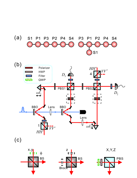
Figure 1: (Color online) $\mathbf{a}$. The two graph states created. $P_{i}$ represents (polarization) qubit $i$, and S1 and S4 represent (spatial) qubits 5 and 6, respectively. $\mathbf{b}$. Scheme of the experimental setup to generate the desired graph states. Femtosecond laser pulses ($\approx$ 200 fs, 76 MHz, 788 nm) are converted to ultraviolet and transmitted through two BBO crystals (2 mm), where two photon pairs are generated. The observed two-fold coincident count rate is about 2.6 $\times$ $10^{4}$/s. Two additional polarizers are inserted into the arms of the second pair to prepare two single photon states. $\mathbf{c}$. The measurement setups for the desired observables. The first setup is for $x$ measurement of spatial qubits when $\phi=0$, and for $y$ measurement of spatial qubits when $\phi=90^{\circ}$. The second one is for $z$ measurement of spatial qubits by using blocks in the two paths of the beam splitter. The third one is for $X,Y,Z$ measurements of polarization qubits by using half wave plates (HWPs), quarter wave plates (QWPs), and PBSs.

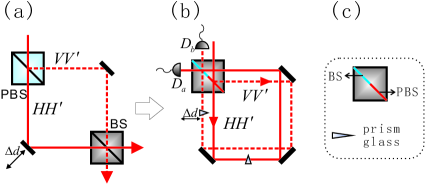
Figure 2: (Color online) Apparatuses of constructing Sagnac-ring interferometer in order to measure all the necessary observables of spatial modes. $\mathbf{a}$. The original scheme of single photon interferometer, which is easily affected by the environment and can be stable for only several minutes. $\mathbf{b}$. Our single photon interferometer in the Sagnac-ring model. Two special prism glasses are inserted to change optical path delay in order to obtain the desired phase. $\mathbf{c}$. A special crystal combining the function of beam splitter and PBS.

III III. results of the state fidelity

In order to measure the states’ fidelities and test the Bell inequalities, we need to implement the desired local measurements. The measurement setups are shown in Fig. 1c, which are similar to Refs. Kai ; Matini1 . Here and in the following, $x$, $y$, $z$ refer to the Pauli matrices for the spatial modes, and $X$, $Y$, $Z$ refer to the Pauli matrices of the polarization modes. The measurements of $x,y$ observables are implemented by overlapping different modes of a photon on a beam splitter (BS), and the measurement of $z$ observable is implemented by blocking one or the other input path of the BS. The observables of polarization qubits are measured by placing a combination of a quarter-wave plate, a half-wave plate and a PBS in front of the single-photon detectors. Although a photon’s polarization and spatial information is read out simultaneously, they are independent measurements and have no influence on each other.

The measurements of spatial modes require single photon interferometers as shown in Fig. 2a. This interferometer is very easily affected by its environment and can only be stable for a few minutes. In our experiment, an ultra-stable Sagnac-ring technique N07 ; A07 is applied to satisfy the required stability. First, we design a crystal combining a PBS and a BS as shown in Fig. 2c. Then, we construct the single photon interferometer in a Sagnac-ring configuration (see Fig. 2b). The $H$-polarized component is transmitted and propagated through the interferometer in the counterclockwise direction, while the $V$-polarized component is reflected and propagated through the interferometer in the clockwise direction. Then, the interference happens when the two components meet at the BS. Such interferometer can be stable for at least ten hours Gao .

To estimate the fidelity of the prepared states, we consider an observable $B$ with the property $\left\langle\phi\right|B\left|\phi\right\rangle\leq\left\langle{\phi}|{Y_{6}}\rangle\langle{Y_{6}}|{\phi}\right\rangle=F_{Y_{6}}$ for any $|\phi\rangle.$ This means $\langle{B}\rangle_{\rm exp}$ is a lower bound of the fidelity of the experimentally produced state gtreview . In the experiment, we have chosen the observable $B$ in Ref.  Y6remark and find $\langle{B}\rangle_{\exp}=0.63\pm 0.04$, clearly exceeding 1/2 and thus proving the genuine 6-qubit entanglement of the state gtreview . The fidelity of the linear-type graph state is above $0.61\pm 0.01$ gao22 , also proving the genuine 6-qubit entanglement.

IV IV. Results of Optimal Bell inequalities

The optimal Bell inequality (i.e., the one having the highest resistance to noise) involving only stabilizing observables for the LC₆ state in the form of Eq. (4) is

$$\langle{\mathcal{B}_{LC6}}\rangle=\langle{(\openone+g_{5})g_{1}(\openone+g_{3})(\openone+g_{2})g_{4}(\openone+g_{6})}\rangle\leq 4,$$ (5)

where $g_{5}=z_{5}Z_{1}$, $g_{1}=x_{5}X_{1}Z_{3}$, $g_{3}=Z_{1}X_{3}Z_{2}$, $g_{2}=Z_{3}X_{2}Z_{4}$, $g_{4}=Z_{2}X_{4}x_{6}$ and $g_{6}=Z_{4}z_{6}$ CGR08 . These $g_{i}$ are stabilizing operators of the linear-type graph state, i.e. the graph state is an eigenstate of all the $g_{i}$ with eigenvalue $+1,$ as one can easily check. This writing of the Bell operator is only a short-hand notation, and the required measurements for the Bell test are the ones which arise after multiplying out $\mathcal{B}_{LC6}$ (see Table 1). As all the terms in the Bell operator are products of stabilizing operators, the cluster state is an eigenstate of all these terms, and the value for the ideal cluster state is the algebraic maximum $\langle{\mathcal{B}_{LC6}}\rangle=16.$

Similarly, the optimal stabilizer Bell inequality for the Y₆ state is CGR08

$$\langle{\mathcal{B}_{Y6}}\rangle=\langle{(\openone+g_{3})g_{1}(\openone+g_{5})(\openone+g_{2})g_{4}(\openone+g_{6})}\rangle\leq 4,$$ (6)

where now $g_{3}=Z_{1}Z_{3}$, $g_{1}=X_{1}X_{3}X_{2}x_{5}$, $g_{5}=Z_{1}z_{5}$, $g_{2}=Z_{1}Z_{2}Z_{4}$, $g_{4}=Z_{2}Z_{4}z_{6}$, and $g_{6}=Z_{4}z_{6}.$ Again, the value for the pure Y₆ state is $\langle{\mathcal{B}_{Y6}}\rangle=16.$

A remarkable feature of these Bell inequalities is that the LC₆ state and the Y₆ state violate local realism by a factor of four, which is also the violation for the six-qubit GHZ state, if only stabilizing elements are considered (the optimal Bell inequality is then the Mermin inequality CGR08 ). However, the LC₆ and Y₆ state are more resistant to decoherence than the GHZ₆ DB04 . In fact, one can directly see that if decoherence acts as a depolarizing channel on each qubit, the violation of the Mermin inequality for the GHZ₆ state decreases faster than for the graph states considered here. Namely, if noise like $\varrho\mapsto p\varrho+(1-p)\openone/2$ is acting on each qubit separately, the value of the Mermin inequality decreases with $p^{6}$, as the Mermin inequality consists only of full correlation terms. In our Bell inequalities, however, half of the terms contain the identity on one qubit (see Tables I and II), which means that they decay only with $p^{5},$ and the total violation decreases like $(p^{6}+p^{5})/2.$ This proves that the non-locality vs. decoherence ratio of GHZ states is not universal: there are states with a similar violation which are more robust against decoherence.

Observable	Value	Observable	Value
$xXZZXx$	$0.61\pm 0.04$	$-xXZZYy$	$0.60\pm 0.04$
$xXIYYx$	$0.63\pm 0.04$	$xXIYXy$	$0.62\pm 0.04$
$-yYZZXx$	$0.55\pm 0.04$	$yYZZYy$	$0.56\pm 0.04$
$-yYIYYx$	$0.65\pm 0.03$	$-yYIYXy$	$0.56\pm 0.04$
$xYYIXx$	$0.58\pm 0.04$	$-xYYIYy$	$0.63\pm 0.04$
$xYXXYx$	$0.58\pm 0.04$	$xYXXXy$	$0.60\pm 0.04$
$yXYIXx$	$0.55\pm 0.04$	$-yXYIYy$	$0.56\pm 0.04$
$yXXXYx$	$0.57\pm 0.04$	$yXXXXy$	$0.60\pm 0.04$

Table 1: Experimental values of the observables on $\left|{LC_{6}}\right\rangle$ required in the test of the optimal Bell inequality. Each experimental value is obtained by measuring in an average time of 400 seconds and considers the Poissonian counting statistics of the raw detection events for the experimental errors. The order of the qubits is 5-1-3-2-4-6.

Observable	Value	Observable	Value
$-XXIYxy$	$0.62\pm 0.04$	$XYIYyy$	$0.59\pm 0.05$
$YYIYxy$	$0.58\pm 0.05$	$YXIYyy$	$0.61\pm 0.05$
$XXIXxx$	$0.56\pm 0.04$	$-XYIXyx$	$0.54\pm 0.04$
$-YYIXxx$	$0.61\pm 0.04$	$-YXIXyx$	$0.63\pm 0.04$
$-YXZXxy$	$0.57\pm 0.05$	$YYZXyy$	$0.62\pm 0.04$
$-XYZXxy$	$0.55\pm 0.04$	$-XXZXyy$	$0.58\pm 0.04$
$-YXZYxx$	$0.54\pm 0.04$	$YYZYyx$	$0.57\pm 0.05$
$-XYZYxx$	$0.59\pm 0.04$	$-XXZYyx$	$0.54\pm 0.04$

Table 2: Experimental values of all the observables on $|Y_{6}\rangle$ for the optimal Bell inequality measurement. Each experimental value is obtained by measuring in an average time of 400 seconds and propagated Poissonian statistics of the raw detection events is also considered. The order of the qubits is 1-3-2-4-5-6.

The experimental results are given in Tables 1 and 2. From these data we find

$$\langle{\mathcal{B}_{LC6}}\rangle_{\rm exp} = 9.40\pm 0.16,$$

$$\langle{\mathcal{B}_{Y6}}\rangle_{\rm exp} = 9.30\pm 0.17,$$ (7)

which violate the classical bound by 34 and 31 standard deviations.

Let us consider the ratio $\mathcal{D}$ between the quantum value of the Bell operator and its bound in LHV theories. Experimentally, we have

$$\mathcal{D}_{LC6}=\langle{\mathcal{B}_{LC6}}\rangle_{\rm exp}/\langle{\mathcal{B}_{LC6}}\rangle_{\rm LHV} = 2.35\pm 0.04,$$

$$\mathcal{D}_{Y6}=\langle{\mathcal{B}_{Y6}}\rangle_{\rm exp}/\langle{\mathcal{B}_{Y6}}\rangle_{\rm LHV} = 2.33\pm 0.04.$$ (8)

These are larger values compared to previous experiments with similar Bell inequalities for four-qubit cluster states: there values of $\mathcal{D}$ from 1.29 to 1.70 have been achieved walther ; Kiesel ; Matini1 ; using a Bell inequality with non-stabilizer observables for the four-qubit GHZ state, $\mathcal{D}=2.22$ has been reached Zhi . To our knowledge, these were the best values obtained so far. Therefore, despite of having a lower fidelity than in the four-qubit experiments, we find a higher violation of local realism, which demonstrates that the amount of nonlocality can increase with the number of qubits. This might help in designing loophole-free Bell inequality tests CRV08 .

We would like to add that the generation of the graph states and the observation of the Bell inequality violations using hyperentanglement implies that some of the qubits are carried by the same photon, and therefore cannot be spatially seperated. So our setup cannot be used to close the locality loophole. However, as the measurements on the polarization qubit and the spatial qubit are independent, such experiments can be viewed as a test of the Kochen-Specker theorem kirchmair ; amselem in order to refute noncontextual hidden variable models.

V V. Conclusion

We have created a Y-shape four-photon six-qubit graph states entangled in the photons’ polarization and spatial modes and proved its genuine six-qubit entanglement. Further, we have implemented two multi-qubit Bell tests based on them, which show the highest violation of Bell inequality so far. It is interesting to investigate the relationship between decoherence and nonlocality further. The aim is to characterize states, which show a high violation of local realism, while being still robust against decoherence.

References

• (1) R. Raussendorf and H.J. Briegel, Phys. Rev. Lett. 86, 5188 (2001); M. van den Nest et al., Phys. Rev. Lett. 97, 150504 (2006).
• (2) D. Schlingemann and R.F. Werner, Phys. Rev. A 65, 012308 (2001); D. Schlingemann, Quantum Inf. Comput. 2, 307 (2002).
• (3) M. Hein, J. Eisert, and H.J. Briegel, Phys. Rev. A 69, 062311 (2004); M. Hein et al., in Quantum Computers, Algorithms and Chaos, edited by G. Casati, D.L. Shepelyansky, P. Zoller, and G. Benenti (IOS Press, Amsterdam, 2006); quant-ph/0602096.
• (4) V. Scarani et al., Phys. Rev. A 71, 042325 (2005); J. Barrett et al., Phys. Rev. A 75, 012103 (2007); O. Gühne and A. Cabello, Phys. Rev. A 77, 032108 (2008).
• (5) A. Cabello and P. Moreno, Phys. Rev. Lett. 99, 220402 (2007).
• (6) A. Cabello, O. Gühne, and D. Rodríguez, Phys. Rev. A 77, 062106 (2008).
• (7) N. D. Mermin, Phys. Rev. Lett. 65, 1838 (1990).
• (8) O. Gühne et al., Phys. Rev. Lett. 95, 120405 (2005); G. Tóth, O. Gühne, and H.J. Briegel, Phys. Rev. A 73, 022303 (2006); L.-Y. Hsu, Phys. Rev. A 73, 042308 (2006).
• (9) P. Walther, M. Aspelmeyer, K. J. Resch, and A. Zeilinger, Phys. Rev. Lett. 95, 020403 (2005).
• (10) N. Kiesel et al., Phys. Rev. Lett. 95, 210502 (2005).
• (11) G. Vallone et al., Phys. Rev. Lett. 98, 180502 (2007).
• (12) Z. Zhao et al., Phys. Rev. Lett. 91, 180401 (2003).
• (13) P. G. Kwiat, J. Mod. Opt. 44, 2173 (1997).
• (14) J. T. Barreiro et al., Phys. Rev. Lett. 95, 260501 (2005).
• (15) G. Vallone et al., Phys. Rev. Lett. 100, 160502 (2008).
• (16) K. Chen et al., Phys. Rev. Lett. 99, 120503 (2007).
• (17) H. S. Park et al., Optics Express 15, 17960 (2007).
• (18) W.-B. Gao et al., Nature Physics, 6, 331 (2010).
• (19) P. G. Kwiat et al., Phys. Rev. Lett. 75, 4337 (1995).
• (20) Z. Zhao et al., Nature (London) 430, 54 (2004).
• (21) D. E. Browne and T. Rudolph, Phys. Rev. Lett. 95, 010501 (2005).
• (22) Y. Tokunaga et al., Phys. Rev. Lett. 100, 210501 (2008).
• (23) W.-B. Gao et al., Phys. Rev. Lett. 104, 020501 (2010).
• (24) T. Nagata et al., Science 316, 726 (2007).
• (25) M. P. Almeida et al., Science 319, 579 (2007).
• (26) O. Gühne and G. Tóth, Phys. Rep. 474, 1 (2009).
• (27) See the online material of C.-Y. Lu et al., Phys. Rev. Lett. 102, 030502 (2009).
• (28) W. Dür and H.-J. Briegel, Phys. Rev. Lett. 92, 180403 (2004).
• (29) A. Cabello, D. Rodríguez, and I. Villanueva, Phys. Rev. Lett. 101, 120402 (2008).
• (30) G. Kirchmair et al. Nature 460, 494 (2009).
• (31) E. Amselem et al. Phys. Rev. Lett. 103, 160405 (2009).