Regression modeling method of space weather prediction

Abstract

A regression modeling method of space weather prediction is proposed. It allows forecasting Dst index up to 6 hours ahead with about $90\%$ correlation. It can also be used for constructing phenomenological models of interaction between the solar wind and the magnetosphere. With its help two new geoeffective parameters were found: latitudinal and longitudinal flow angles of the solar wind. It was shown that Dst index remembers its previous values for 2000 hours.

Keywords space weather; prediction; forecasting; magnetic storms; statistics; regression

1 Introduction

The humankind studies space weather for more than 4000 years starting from the first mentions of auroras in ancient Chinese literature. The term “space weather” itself exists for almost a century. The official definition adopted by COSPAR states that “Space weather describes the physical processes induced by solar activity that have impact on our terrestrial and space environment, on ground based and space technological systems, and on human activities and health.” The first part of this definition actually covers two spatial scales of space weather, because when we speak about space weather in space, e.g. in connection with spacecraft failures, we usually mean some local parameters of the environment, and when we speak about space weather on the Earth, e.g. in connection with human health, we usually mean some integral characteristics like the geomagnetic indices. Since this article centers on the variations of the geomagnetic field, the latter meaning will be used. The second part of this definition indicates practical manifestations of space weather. The impact of the space weather on technological systems is generally accepted (see Marubashi (1989)) due to a number of spectacular events like the superstorm of 1989 when Canada’s power grid was disabled for 9 hours and numerous spacecraft failures due to “killer electrons” causing arcing in electronic components, see Romanova et al. (2005). The impact on human health, however, is disputed by most specialists. Nevertheless, the latest reports (e.g. Khabarova & Dimitrova (2008), Stoupel et al. (2006)) indicate that there is indeed a strong correlation between the rate of sudden cardiac deaths and the space weather.

The space weather problem is twofold. The first aspect is purely practical and aims for prediction and, eventually, mitigation of adverse effects of space weather. Ideally, this task should be accomplished by launching a vast number of spacecraft which will monitor the Sun-Earth region for large-scale structures like CMEs. Unfortunately, the resources of the humankind are insufficient to produce and maintain such a large space fleet as well as to process all the data delivered by these spacecraft. So, today we should use the resources at hand, which include a few solar wind spacecraft (ACE, WIND, SOHO, and STEREO), magnetospheric spacecraft (CLUSTER, THEMIS), and ground-based stations (Intermagnet, MAGDAS, etc.), to develop forecast techniques that will be used in future. Thus, we should try to predict space weather with what data we have, and we should aim for possibly longer prediction times to allow for some kind of countermeasures.

The second aspect is mostly academic and involves study of the processes in the near-Earth space and, specifically, understanding of interaction between the solar wind and the magnetosphere. Naturally, improving our knowledge of the underlying physics significantly improves predictive capabilities, so fulfilling the second task will significantly help with the first one. Modern conceptions of solar wind-magnetosphere interaction are mostly based on phenomenological models constructed in 1960’s. However, there are numerous problems these models cannot answer. This is largely due to the fact that these models were developed at the very beginning of the space era when data quality and quantity were immeasurably worse than today. For more than 40 years we collected astonishing amounts of data about solar wind parameters and geomagnetic activity and now it is time to put them to good use.

2 Possible approaches to space weather prediction

Space weather prediction is a challenging and nontrivial activity, see Li et al. (2003). The most straightforward approach to space weather prediction is studying the whole complex chain of physical processes involved in magnetospheric dynamics and conjugating them in a global model of the evolution of the magnetosphere under the influence of the solar wind. Unfortunately, this is not yet possible due to our poor understanding of the physics of the interaction between the solar wind and the magnetosphere. For this reason, different approaches should be tried.

According to Khabarova (2007), today there are several established methods of space weather prediction, listed below.

1. Morphological analysis of solar images.

This method provides the longest prediction time (up to a week). Its accuracy is unknown since it is used for the academic purposes only. Today it is purely manual and thus almost useless for practical implications.

2. Detection of large-scale perturbations in the solar wind, see e.g. Eselevich & Fainshtein (1993), Eselevich et al. (2009).

This method provides a very good prediction time (up to several days), but is capable of predicting less than 10% of the most intense storms. While it is very inaccurate when used alone, it can prove to be useful in combination with one of the following short-term methods.

3. Construction of empirical models, see e.g. Burton et al. (1975), Valdivia et al. (1996), O’Brien & McPherron (2000a), O’Brien & McPherron (2000b), Temerin & Li (2002), Temerin & Li (2006), Ballatore & Gonzalez (2003), Cid et al. (2005), Siscoe et al. (2005).

This method provides the shortest prediction time (up to 1 hour) with moderate accuracy ($\sim 70\%$). Potentially this method could demonstrate far better results if the physics behind the magnetic storms was less of a mystery.

4. Numerical modeling, see e.g. Liu et al. (2008), McKenna-Lawlor et al. (2008).

This method provides a good prediction time (up to several days) but its accuracy varies in huge limits. The accuracy of these methods is limited by their inability to correctly describe plasma instabilities. Besides, the ring current can not be described in the framework of ideal MHD, which forms the basis of most numerical models. However, they can adequately describe the motion of e.g. magnetic clouds in the interplanetary environment, but rely on different methods to detect them.

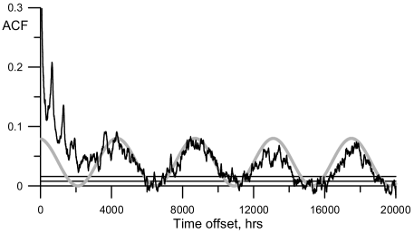
Fig. 1 : Autocorrelation function of Dst. Horizontal lines correspond to top and mean incidental correlation levels in abscence of periodic variations. Gray sine has a period of 1/2 year and depicts seasonal variations

Fig. 2 : Distribution of correlation coefficient of Dst at very large time offsets in abscence of periodic variations

Fig. 3 : Dependence of Fisher significance $F$ of the corresponding term in equation (1) on the time offset for the $1^{h}$ autocorrelation model

5. Multidimensional time series analysis.

This method provides a moderate prediction time (up to several hours) with the highest accuracy ($>80\%$). They are very effective and easy to use but strongly depend on satellite data availability. These are “black box” or “input-output” models, which seek only to reproduce the system’s output in response to changes of its inputs. The model terms are usually physically interpretable and thus useful for construction of new phenomenological models. For this reason, this method can not only provide space weather forecast per se, but also can improve our knowledge of the physics involved and thus increase the efficiency of other methods.

Further we shall speak about the last method, keeping in mind that its results can be used later to assist other methods. First of all, let us discuss its existing implementations.

Multidimensional time series analysis can be performed using the methods of statistics, signal processing, informatics, fuzzy logic etc. The most widely used variations are artificial neural networks (e.g. Kugblenu et al. (1999), Watanabe et al. (2002), Wing et al. (2005), Pallocchia et al. (2006)), optimization (e.g. Zhou & Wei (1998), Balikhin et al. (2001), Harrison & Drezet (2001)), and correlation analysis (e.g. Rangarajan & Barreto (1999), Oh & Yi (2004), Wei et al. (2004), Johnson & Wing (2004), Johnson & Wing (2005)). Neural network approach provides short-term predictions up to 4 hours with the correlation coefficient of 0.79 in the paper by Wing et al. (2005). Earlier implementations of this approach experienced significant difficulties predicting strong geomagnetic storms with $Kp>5$, but this approach remains one of the most popular alongside the empirical methods. Optimization approach seems to be more successful being able to provide 8-hour predictions in the paper by Harrison & Drezet (2001). However, in the papers based upon the optimization methods the volume of the dataset used is insufficient to correctly describe secular variations of geomagnetic activity. Correlation analysis gives interesting results, but it was used solely for developing and constraining empirical models (see Johnson & Wing (2004)). However, most of these methods have a common feature: they lead to a regression relationship at some point, so it seems natural to skip all the preliminary steps and instantly use the regression analysis without unnecessary multiplication of entities. Regression analysis itself was attempted earlier by Srivastava (2005), but it was used to estimate the probability of intense/super-intense storm occurence depending on the solar and interplanetary parameters. Srivastava (2005) was able to predict 2 of 4 super-intense and 5 of 5 intense CME driven storms during the 1996-2002 period using another 46 CME driven storms to train his model.

Hereafter we propose a new approach, named “regression modeling”, which already allows achieving accurate ($\sim 90\%$) 6 hours ahead forecast of the Dst index, which we will use as a quantitative characteristics of space weather. This method can be easily extended to predict other geomagnetic indices like Kp or Ap.

3 Description of the regression modeling method

The proposed method is statistical, but has some features of empirical models. It is based upon the regression analysis and the mathematical statistics. In its framework the predicted Dst value is sought in the form

$$D_{st}(j+k)=\sum\limits_{i}{C_{i}x_{i}(j)},$$ (1)

where $j$ is the number of current step (number of hours since Jan 1, 1963), $k$ is the prediction length, $C_{i}$ are the regression coefficients, and $x_{i}$ are the regressors, which are functions and combinations of input quantities, which are already measured at the time when prediction is made. Values of $C_{i}$ are determined by least square method (LSM) over a large sample of solar wind and geomagnetic data (see next chapter), with equal statistical weights of all points. The statistical significance of the regressors was determined by Fisher test (F-test) (see Fisher (1954), Hudson (1964)). This test allows separating significant and insignificant regressors. The insignificant parameters are then rejected and the routine is repeated until the regression contains only significant regressors. Of course, this method does not guarantee that all the significant regressors will enter the regression, but physical considerations and brute force in the form of trial and error provide us with requested reliability. The regressors $x_{i}$ are generally nonlinear, so from the control theory’s point of view, this method is able to describe discrete dynamical systems with strong nonlinearity. This is an essential feature of the regression modeling method.

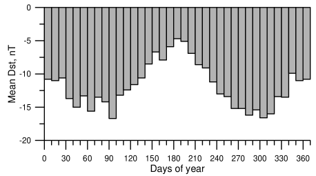
Fig. 4 : Seasonal variation of Dst

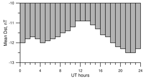
Fig. 5 : Diurnal variation of Dst

Fig. 6 : Sum of terms directly describing seasonal variation of Dst

Fig. 7 : Sum of terms directly describing diurnal variation of Dst

There is only one manual operation in this method – selection of regressors to be considered. For this purpose all known models, basic physical considerations, and random choice are used. Naturally, common sense also counts: for example it would be silly to add IMF components in GSE and GSM coordinates at the same time. If some regressors $x_{i}$ appeared to be statistically significant, we also checked the significance of products of their powers $\prod\limits_{i}{x_{i}^{p_{i}}}$, where $p_{i}$ can be any real number, including zero, but for practical purposes we used integer values of $p_{i}$ in the range from 0 to 6. This yields a very important feature of the regression analysis: it allows checking the statistical significance of any regressor, which can be useful for verifying different physical hypotheses. In this sense we will call a parameter “geoeffective” if it appears at least in one statistically significant regressor.

More details of this method can be found in the article Parnowski (2009a).

4 Data and routine

The OMNI2 (2009) database was used. It contains IMF, solar wind and geomagnetic data, averaged over 1-hour intervals (49 parameters in total, starting from Jan 1, 1963). It was supplemented with provisional Dst data, taken from WDC for Geomagnetism (Kyoto). Thus a continuous 44-year Dst time series was obtained.

We estimated the geoeffectiveness of a parameter by coefficients and statistical significances of all regressors, which contain this parameter. This was done in the following way. After processing the data with the least square method, Fisher significance parameter $F$ was determined for each regressor. All the $F$ values were compared to the values 2.7055, 3.84, 5.02, 6.635, 7.879, 10.83 and 12.1, which correspond to statistical significance of 90, 95, 97.5, 99, 99.5, 99.9 and 99.95% respectively. Then, insignificant regressors were rejected and the routine was repeated until all the regressors were significant. The number of significant regressors depends on the selected significance threshold. All results given herein correspond to the significance threshold of 90%. In contrast to empirical models we do not add fitting parameters and all the regressors have physical meaning. The described routine was applied to the sample, obtained from the initial dataset after rejecting filled values. This sample can be divided into two subsamples, corresponding to quiet ($Dst>-50nT$) and perturbed ($Dst\leq-50nT$) conditions.

First, we determined which previous Dst values are statistically significant. For this purpose, we constructed an autoregression (see details in Parnowski (2009b))

$$Dst(j+k)=C_{0}+\sum\limits_{i=1}^{N}{C_{i}Dst(j-i+1)},$$ (2)

where $N$ is the “age” of the oldest Dst value. This model alone is not sufficient to correctly predict Dst, but it sets a basis for the construction of models that are able to do so. Let us determine the maximum reasonable value of $N$. For this purpose, we plot the autocorrelation function (ACF) of the Dst index for $k=1$ (see Fig. 1). One can see that ACF tends to a sinusoid with a period close to half a year. This is caused by seasonal variations. This yields a question: if there were no temporal variations, what would ACF tend to at large offsets? If the distribution of Dst was normal, the answer would be zero. However, the distribution is not normal, so ACF can tend to some non-zero quantity. To determine this quantity we need to remove temporal variations. For this purpose we need to calculate the ACF of a random sample with the same statistical characteristics as the Dst sample. The easiest way to get such a sample is to process the Dst sample with a permutation method, which is widely used for determination of correlation functions, e.g. in astronomy. This method is based on random shuffle of the sample. Using this method many times (10000 times in our case) and calculating the correlation coefficient each time, we get the distribution of the correlation coefficient by Monte-Carlo method. The distribution of the correlation coefficient for this sample (Fig. 2) appeared to be very close to a normal distribution with mean 0.008 and variance $5.1\cdot 10^{-6}$. The maximum recorded value in 10000 trials was equal to 0.015. The top and the mean values are depicted on Fig. 1 by horizontal lines. As one can see on Fig. 1, in reality the correlation coefficient exceeds this value at most times due to temporal variations. The ACF crosses the top line for the first time at $\sim 6000$ hours, though the difference between the ACF and the sine with a half-year period crosses it at $\sim 2000$ hours, which is about 3.5 27-day periods, so we will assume the latter value as a rough estimation of $N$. This hints that rather old Dst values can be quite significant. Besides the half-a-year periodicity one can also notice the 27-day periodicity, caused by Carrington rotation of the Sun, which can be taken into account by adding the sunspot number $R$ to the regression.

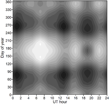
Fig. 8 : Temporal variation of Dst. Darker spots correspond to lower values

Let us return to equation (2). Applying the F-test we can determine which previous Dst values are statistically significant (see Fig. 3). We did not search statistically significant Dst values for $N>900$, but it is possible that there are even older statistically significant values. A similar situation was reported by Johnson & Wing (2004) regarding Kp: ”the significance is often quite large for extended periods of time (10-20 days)”. As our analysis shows, Dst index can “remember” its previous values for significantly longer periods of time. In fact, after adding regressors, corresponding to satellite data, some of the previous Dst values become insignificant. We found that after the addition of these regressors there are still statistically significant values as far as 801 hours ago (33 days and 9 hours) for $k=1$. The statistical significance of this oldest value is over 99.9%.

At this point we already have a large number of regressors, describing just the previous Dst values (autoregression), without satellite data and nonlinear terms. If we add those, the number of regressors will only increase.

After determining which previous Dst values are statistically significant, we added all the solar wind parameters available in the OMNI 2 database. Then, we added nonlinear terms as discussed in Section 3. After adding a new regressor, all the significances are recalculated, and some of the old regressors can become insignificant. The total number of regressors is about 150-200. Since it is very large, we will not give here any lists of regressors or coefficients even for the simplest case $k=1$, but the preliminary list is given in the paper Parnowski (2008).

5 Identification of new geoeffective parameters

In this section we will demonstrate how this method can be used for identification of geoeffective parameters. We will use four parameters as an example: DOY (day of the year), UT (universal time) and latitudinal and longitudinal flow angles of the solar wind.

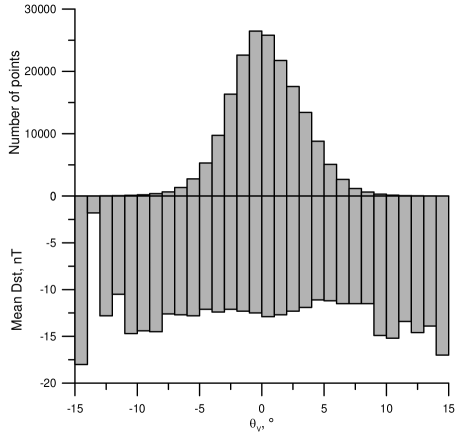
Fig. 9 : Distribution of the latitudinal flow angle and the corresponding mean Dst values

Fig. 10 : Sum of terms describing the latitudinal flow angle

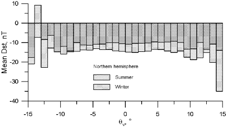
Fig. 11 : Seasonal dependence of latitudinal flow angle’s input in Dst

On Fig. 1 one could see a clear seasonal dependence of the Dst index. This dependence was described in many articles, for example by O’Brien & McPherron (2002), Lyatsky et al. (2001), Takalo & Mursula (2001), and Cliver et al. (2000), but the reason behind it is still disputed. Most authors believe these asymmetries are caused by either of two cusps turning to the sunlit side due to annual rotation of the Earth with respect to the Sun. However, O’Brien & McPherron (2002) state that this mechanism would give only 17% of observed asymmetry. Takalo & Mursula (2001) connected the diurnal variations of Dst with an uneven distribution of Dst network stations. Let us use this known effect to validate our method.

If we select two subsamples, corresponding to summer and winter in northern hemisphere, bounded by vernal and autumnal equinoctia, and verify the hypothesis that the difference between the corresponding average Dst values is statistically significant using a one-sided Student test, we obtain $t_{\infty}=80.264$, which is well over 99.95% significant. Values of $t_{\infty}$ corresponding to 99 and 99.95% significance levels are equal to 2.334 and 3.31 respectively. For diurnal asymmetry Student test gives $t_{\infty}=8.774$, which corresponds to significance level of more than 99.95%. Note that formally Student test is applicable when Dst is normally distributed. In fact, the distribution of Dst is slightly asymmetric, but taking into account the obtained values of $t_{\infty}$, we can be sure in qualitative conclusions made. Figs. 4 and 5 show the histograms of seasonal and diurnal variations of Dst index.

Taking this known geoeffective factor as an example we demonstrate how easily one can take it into account using regression approach. To do so one should simply add terms $a_{1}(j)=\sin((j-1920)\pi/4383)$ and $a_{2}(j)=\cos((j-1920)\pi/4383)$ into the regression. Here $j$ is once again the number of hours since Jan 1, 1963, 1920 is the number of hours between the beginning of the year and the vernal equinox, and 4383 is the number of hours in half a year. The first of these terms is significant and describes summer/winter asymmetry, and the second one (which appears statistically insignificant) describes an absent spring/autumn asymmetry. Likewise, for diurnal asymmetry the corresponding terms will be $b_{1}(j)=\sin((j-2)\pi/12)$ and $b_{2}(j)=\cos((j-2)\pi/12)$. Here 2 is the time difference between UT and the northern geomagnetic pole, and 12 is the number of hours in half a day. Both these terms are significant.

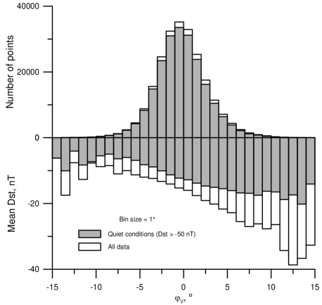
Fig. 12 : Distribution of the longitudinal flow angle and the corresponding mean Dst values. Grey columns correspond to quiet conditions, white columns – to all data

The coefficient of the $a_{1}(j)$ term is 30 times less than the observed difference between mean Dst values of summer and winter subsamples. This can be explained in the following way: there are other regressors, which depend on parameters with statistically significant summer/winter asymmetry, e.g. previous Dst values. They provide the lion share of summer/winter asymmetry of Dst. A good example of such a regressor is the sunspot number $R$, which describes the 27-day periodicity. Nevertheless, there is a small difference which can not be expressed with these terms. Including it into regression, we obtain these statistically significant regressors. To further illustrate this point, let us consider as an example a value $X=const+A\sin\omega t$. In the regression it will look like $X_{n+1}=X_{n}+A\left[\sin\omega(t+\Delta t)-\sin\omega t\right]=X_{n}+A\left[(\cos\omega\Delta t-1)\sin\omega t+\cos\omega t\sin\omega\Delta t\right]$. The first term in brackets is of order $(\omega\Delta t)^{2}$, and the second – $\omega\Delta t$ in the natural assumption that $\omega\Delta t\ll 1$. So, it will seem that the coefficient is $A\omega\Delta t$ rather than $A$. Note that this is just an example and has nothing to do with actual regressors.

Fig. 13 : Sum of terms describing the longitudinal flow angle

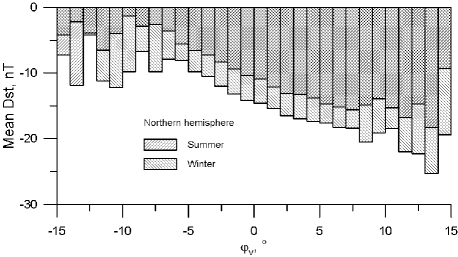
Fig. 14 : Seasonal dependence of longitudinal flow angle’s input in Dst

However if we look on the distribution of mean Dst values vs. time of the year (Fig. 4), we see a much more complicated pattern of seasonal variations of geomagnetic activity. Among other features there is a strong asymmetry between summer and winter on one side and spring and autumn on the other. To take it into account we introduced additional terms into our regression, which are powers of $a_{1}(j)$ and their products with powers of $a_{2}(j)$. The sum of regressors with the corresponding coefficients, depicted on Fig. 6, is very similar to Fig. 4. Note that Fig. 6 was obtained independently from Fig. 4.

We did the same thing with the diurnal asymmetry. The distribution is plotted on Fig. 5, and the sum of regressors with the corresponding coefficients – on Fig. 7. The term $a_{1}(j)\cdot b_{1}(j)$ is also significant and should be included in the regression. After this we obtained a joint distribution of semiannual and diurnal variations of Dst index, plotted on Fig. 8. It contains 18 regressors. Increasing the number of regressors describing temporal variations of geomagnetic activity we can improve the accuracy of this distribution. In particular, one could add 11-year and 22-year solar cycles, higher powers of $a_{i}(j)$ and $b_{i}(j)$ etc.

Thus, we demonstrated how easily one can take into account new geoeffective parameters in this method’s framework.

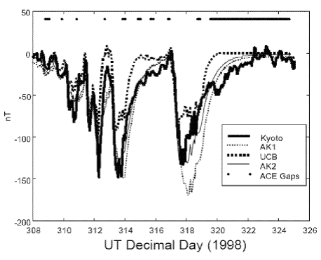
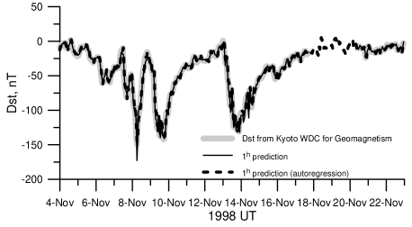
Fig. 15 : Comparison between predictions results of O’Brien & McPherron (2000a) (top) and ours (bottom) 1 hour ahead. The following designations are used: ’Kyoto’ – official Dst index, available at Kyoto WDC for Geomagnetism; ’AK1’ – prediction based on the model of Burton et al. (1975) with re-calculated coefficients; ’UCB’ – prediction based on the model of Fenrich & Luhmann (1998); ’AK2’ – prediction based on the model of O’Brien & McPherron (2000b); ’ACE Gaps’ refer to the top line, indicating the availability of solar wind data measured by ACE satellite

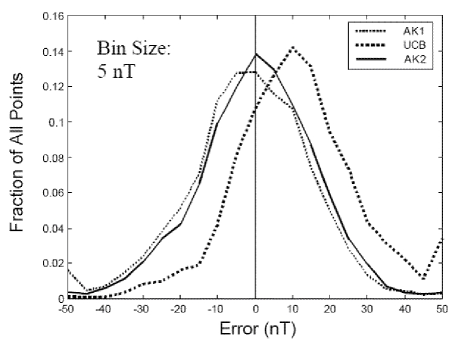
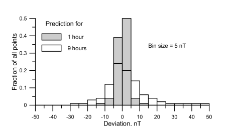
Fig. 16 : Error charts of predictions results of O’Brien & McPherron (2000a) (top) and ours (bottom) 1 hour ahead. Error chart for our 9 hour prediction is plotted for reference

Now let us discuss parameters, whose geoeffectiveness was determined by this method, and demonstrate that they are indeed geoeffective.

Latitudinal flow angle $\theta_{V}$ was mostly associated with the southern component of IMF. I plotted the distribution of its value and the corresponding mean Dst value on Fig. 9. The distribution looks similar to a normal distribution, but it significantly differs from the normal one according to $\chi^{2}$ test. This manifests in much larger number of points with deviations more than $\sigma$ than follows from the normal distribution. This is mostly caused by the number of points in the wing bins $\left|\theta_{V}-\left<\theta_{V}\right>\right|>4\sigma$ being equal to 196 points versus 11 points in the case of normal distribution. However, most of these points were obtained in the 1960s, when quality of measurements was much worse then today. This period includes the maximum and minimum values of $\theta_{V}$, equal to $-59.7^{\circ}$ and $18.8^{\circ}$. Nevertheless, these points constitute only a minor fraction of all points and didn’t affect the linear regression routine. Assuming normal distribution we obtain $\sigma=2.925$ and $\left<\theta_{V}\right>=0.27<0.1\sigma$. Thus, the distribution is insignificantly shifted towards positive values.

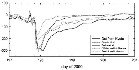
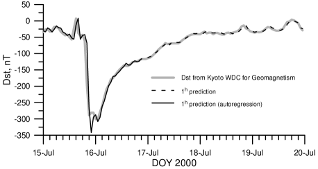
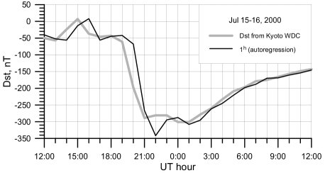
Fig. 17 : Comparison between predictions results of Cerrato et al. (2004), Burton et al. (1975), O’Brien & McPherron (2000a), Fenrich & Luhmann (1998) (top) and ours (middle) 1 hour ahead. Bottom plot is a scaled up version of the middle one

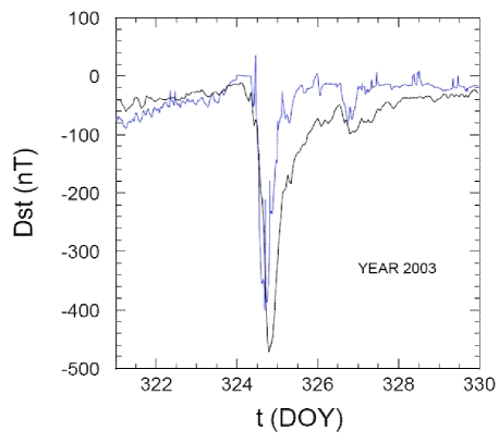
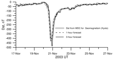
Fig. 18 : Comparison between predictions results of Pallocchia et al. (2006) (top) and ours (bottom) 1 hour ahead. Our 3-hour prediction is given for reference. On the top plot black line depicts Dst from Kyoto WDC, and the blue line – 1 hour prediction

If we ignore the wing bins in the distribution of mean Dst values against $\theta_{V}$, which are somewhat random due to small amount of points in them, we will notice a slight almost linear trend. If we plot the sum of terms containing $\theta_{V}$ (Fig. 10), we will notice a similar trend. If we select two subsamples, one $-8<\theta_{V}<-5$ and other $4<\theta_{V}<9$, and verify the hypothesis that the difference between the corresponding average Dst values is statistically significant using a one-sided Student test, we obtain $t_{\infty}=6.278$, which is over 99.95% significant.

If we divide the sample in two subsamples: one for northern summer and one for northern winter, we obtain such a picture (Fig. 11). Once again, let us not look at the wing bins. What do we see? Summer distribution has an obvious linear trend, but the winter one has not. If we apply the Student test to the same intervals now, we obtain that $t_{\infty}$ is 5.44 in the summer and only 0.059 in the winter. The prior corresponds to more than 99.95% significance, while the latter – to less than 10%. This could mean that there are two factors connected with the latitudinal flow angle, which work together in the summer and against each other in the winter. The physical explanation of this phenomenon, however, lies beyond the scope of this paper.

Longitudinal flow angle $\varphi_{V}$ was only occasionally used in models. However, it appeared to be even more significant than the latitudinal flow angle. Its distribution together with corresponding mean Dst values is plotted on Fig. 12, where white bars show the complete dataset sans rejects, and the grayed bars show the quiet-time sample with $Dst>-50nT$. Like the latitudinal flow angle, the distribution of the longitudinal flow angle resembles normal distribution. However, $\chi^{2}$ test disproves the relevant null-hypothesis. Once again, this is mostly due to wing bins which are mostly formed of data points, corresponding to measurements in 1960s, including maximum and minimum values equal to $-65.6^{\circ}$ and $48.5^{\circ}$. Assuming normal distribution we obtain $\sigma=2.934$ and $\left<\varphi_{V}\right>=-0.30\approx-0.1\sigma$.

A significant trend is the most prominent feature of this figure. If we plot a sum of regressors, which contain $\varphi_{V}$ (Fig. 13), we see a very similar trend. Like before, we plot the distribution for summer and winter subsamples separately (Fig. 14). We see that the trend is identical on both plots, so the corresponding effect is season-independent. The list of regressors for $k=1$, containing $\theta_{V}$ and $\varphi_{V}$, is given in Table 1. It contains the regressors themself, their coefficients and $F$ values.

Thus, we demonstrated that our method is truly capable of pointing out new geoeffective parameters and verified the geoffectiveness of two such quantities.

6 Prediction results

Table 1 : Regressors containing the flow angles. $V(j)$ is the bulk flow velocity of the solar wind

$i$	$x_{i}$	$C_{i}$	$F_{i}$
$1$	$\theta_{V}(j)\cdot V(j)$	$\phantom{-}(2.8\pm 0.9)\cdot 10^{-5}$	$10.2$
$2$	$\theta_{V}^{4}(j)$	$(-4.9\pm 1.2)\cdot 10^{-5}$	$17.5$
$3$	$a_{1}(j)\cdot\theta_{V}(j)\cdot D_{st}(j)$	$\phantom{-}(1.3\pm 0.3)\cdot 10^{-3}$	$18.7$
$4$	$a_{1}(j)\cdot\theta_{V}^{4}(j)$	$(-3.2\pm 1.6)\cdot 10^{-5}$	$\phantom{0}4.0$
$5$	$\varphi_{V}(j)$	$(-4.1\pm 0.6)\cdot 10^{-2}$	$50.1$
$6$	$\varphi_{V}^{2}(j)$	$(-4.5\pm 1.5)\cdot 10^{-3}$	$\phantom{0}9.3$
$7$	$\varphi_{V}^{3}(j)$	$(-3.5\pm 1.3)\cdot 10^{-4}$	$\phantom{0}7.1$
$8$	$\varphi_{V}^{4}(j)$	$\phantom{-}(5.3\pm 1.7)\cdot 10^{-5}$	$10.1$
$9$	$a_{2}(j)\cdot\varphi_{V}(j)$	$(-2.2\pm 0.8)\cdot 10^{-2}$	$\phantom{0}7.9$
$10$	$a_{2}(j)\cdot\varphi_{V}^{3}(j)$	$\phantom{-}(5.1\pm 1.9)\cdot 10^{-4}$	$\phantom{0}7.6$
$11$	$a_{2}(j)\cdot\varphi_{V}^{4}(j)$	$(-3.5\pm 1.4)\cdot 10^{-5}$	$\phantom{0}6.6$

Table 2 : Statistical characteristics of forecasting models

$k$, h	RMS, nT	LC	PE	Note
$1$	$3.76$	$\vphantom{\sum\limits{}}\frac{0.987}{0.977}$	$0.975$
$1$	$4.50$	$\vphantom{\sum\limits{}}\frac{0.982}{0.977}$	$0.964$	autoregression
$1$	$3.15$	$\vphantom{\sum\limits{}}\frac{0.977}{0.958}$	$0.983$	$Dst>-50nT$
$1$	$6.25$	$\vphantom{\sum\limits{}}\frac{0.984}{0.963}$	$0.931$	$Dst\leq-50nT$
$3$	$7.60$	$\vphantom{\sum\limits{}}\frac{0.941}{0.906}$	$0.899$
$6$	$10.45$	$\vphantom{\sum\limits{}}\frac{0.882}{0.813}$	$0.809$
$9$	$12.84$	$\vphantom{\sum\limits{}}\frac{0.820}{0.727}$	$0.711$
$12$	$14.47$	$\vphantom{\sum\limits{}}\frac{0.764}{0.662}$	$0.636$	for reference
$18$	$16.72$	$\vphantom{\sum\limits{}}\frac{0.677}{0.554}$	$0.514$	for reference
$24$	$18.22$	$\vphantom{\sum\limits{}}\frac{0.605}{0.505}$	$0.423$	for reference

Taking into account the considered parameters together with parameters, whose geoeffectiveness was beyond doubts, like previous values of Dst, dawn-dusk electric field, ram pressure of the solar wind and most of other parameters from the OMNI2 database, we constructed models for predicting Dst 1, 3, 6, 9, 12, 18, and 24 hours ahead, and 3 more models for predicting Dst 1 hour ahead for quiet and perturbed conditions and for the case when satellite data are unavailable (autoregression, see more in Parnowski (2009b)). The statistical characteristics of these models are summarized in Table 2. They include Residual Mean Square (RMS), Linear Correlation Coefficient (LC), and Prediction Efficiency ($PE=1-RMS^{2}/SD^{2}$, where SD is the sample’s Standard Deviation). In divided cells the top number corresponds to the actual model, and the bottom one – to the simplest possible model $D_{st}(j+k)=D_{st}(j)$. It is noteworthy that despites good correlation for all the models, in reality only the 1-hour and 3-hour models are ready for practical use, and the 6-hour model can potentially reach this state. This is due to a significant time shift being present in further predicting models.

Note that since the proposed method is statistical, there is little difference whether the “training” sample contains the period when prediction is made (“test” sample) or not. To further illustrate this point let us consider an example: I predicted Dst 3 hours ahead using the “test” sample from 2007 to 2008 and 3 “training” samples: the sample from 1976 to 2003 gives LC=0.851, the sample from 1976 to 2006 gives LC=0.854, and the sample from 1976 to 2008 gives LC=0.854 as well. The first two “training” samples do not contain the “test” sample, but the results are slightly different. The third “training” sample contains the “test”sample, yet the result is the same as for the second sample. This yields a conclusion that the volume and statistical properties of the “training” sample affect the prediction results stronger than the inclusion of the “test” sample. So, the inclusion of the “test” sample to the “training” sample has little or no effect on the LC. PE is calculated independently from the “test” sample and is not affected by its selection in any way.

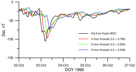
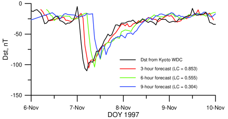
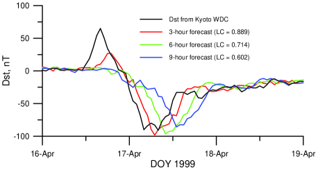
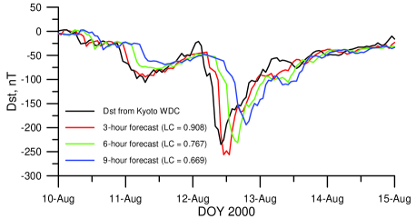
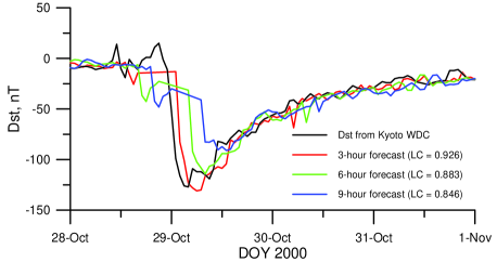
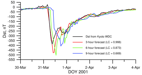
1234567890

Fig. 19 : Prediction results for some specific intervals

We also present graphical representations of prediction in comparison with results of other authors: O’Brien & McPherron (2000a) (Fig. 15, 16), Cid et al. (2005) (Fig. 17), and Pallocchia et al. (2006) (Fig. 18). Note, that the intervals for prediction were selected by authors of the original papers, and the coefficients in eq. (1) were the same all the time and for all the figures. It is clearly visible that our method provides much more precise forecast than most empirical models and typical neural network models. Ridiculously, even our $9^{h}$ model is more precise than most empirical $1^{h}$ models. The autoregression model, described by eq. (2), though, lags in the left part of the plot due to a rapid positive change of Dst at 1500 UT. The lag persists through the growth phase and the main phase, and vanishes only in the recovery phase. For this reason, the autocorrelation model holds little practical value and should be considered as a transitional result, required to construct the full model. It is, however, possible to improve it by adding terms describing temporal variations, and, for example, the number of sunspots, but then the term “autoregression” will no longer be applicable.

On Fig. 19 we present the results of prediction 3, 6 and 9 hours ahead for a number of events, kindly selected for us by V.G. Fainshtein, which are particularly hard to predict by medium-term methods, such as Eselevich et al. (2009), to verify the efficiency of our method. We can see that this method’s accuracy is higher for stronger storms, which are of greater interest. A huge advantage of this method is that the most resource-demanding operation – the calculation of the regression coefficients – should be performed only once for each model. The prediction itself is just a summation of a polynom, which usually takes no more than 4-6 seconds on an average PC (including disk I/O), which allows for creation of fully automated operational on-line space weather forecast services.

7 Conclusion

The proposed regression approach appeared to be more than adequate for space weather forecasting. For the forecasting per se, its main advantages are quite good correlation (about 90% for 6 hours forecast), adaptability to any samples, and very fast forecasting code (typically about 5 seconds on an average PC). For the identification of geoeffective parameters it is extremely convenient and easy to use. In particular, it allowed to uncover 2 new geoeffective parameters – the latitudinal and the longitudinal flow angles of the solar wind.

This is just a short summary of the regression modeling method, since its full description would take much more space. Of course, this method can be used in conjunction with other methods, first of all, with physical methods of detection of large-scale perturbations in the solar wind and with empirical models.

Acknowledgements The author would like to thank Prof. O.K. Cheremnykh, Prof. V.A. Yatsenko, and Academician V.M. Kuntsevich for fruitful discussion, Prof. V.G. Fainshtein for useful remarks and for providing a list of geomagnetic events for validation of the model, and Reviewer #1 for valuable comments which greatly improved this article.

The author is grateful to the Space Physics Data Facility (SPDF) and the National Space Science Data Center (NSSDC) for the free online OMNI2 catalogue and to the World Data Center for Geomagnetism (WDC-B) at Kyoto University for the free online catalogue of geomagnetic indices.

This work was partially supported by the National Academy of Sciences of Ukraine, state programme “GEO-UA”, and by the National Space Agency of Ukraine, state contract No. 8-09/08 “Programa-N”.

References

- Balikhin et al. (2001) Balikhin, M.A. et al. 2001, Geophys. Res. Lett., 28, 1123
- Ballatore & Gonzalez (2003) Ballatore. P. & Gonzalez, W.D. 2003, Earth Planets Space, 55, 427
- Burton et al. (1975) Burton, R.K. et al. 1975, J. Geophys. Res., 80, 4204
- Campbell (1996) Campbell, W.H. 1996, J. Atm. & Terr. Phys., 58, 1171
- Cerrato et al. (2004) Cerrato, Y. et al., 2004, in “Lecture notes and essays in Astrophysics”, pp.131-142
- Cid et al. (2005) Cid, C. et al., 2005, in Solar Wind 11 – SOHO 16 Workshop, “Connecting Sun and Heliosphere”, pp.116-119
- Cliver et al. (2000) Cliver, E.W. et al. 2000, J. Geophys. Res., 105, 2413
- Eselevich & Fainshtein (1993) Eselevich, V.G. & Fainshtein, V.G. 1993, Annales Geophysicae, 11(8), 678
- Eselevich et al. (2009) Eselevich, V.G. et al., 2009, Cosmic Research, 47(2), 95
- Fenrich & Luhmann (1998) Fenrich, R.R. & Luhmann, J.G. 1998, Geophys. Res. Lett., 25, 2999
- Fisher (1954) Fisher, R.A., 1954, “Statistical methods for research workers”, Oliver and Boyd: London
- Harrison & Drezet (2001) Harrison, R.F. & Drezet, P.M., 2001, in Les Woolliscroft memorial Conf., “Multipoint measurements versus theory”, pp.141-146
- Hudson (1964) Hudson, D.J., 1964, “Statistics Lectures on Elementary Statistics and Probability”, CERN: Geneva
-
Johnson & Wing (2004)
Johnson, J.R. & Wing, S. 2004, Report PPPL-3919rev.
http://www.pppl.gov/pub_report/2004/PPPL-3919rev.pdf -
Johnson & Wing (2005)
Johnson, J.R. & Wing, S. 2005, J. Geophys. Res.,
doi:10.1029/2004JA010638 - Joselyn (1998) Joselyn, J.A. 1995, Rev. Geophys., 33, 383
- Khabarova (2007) Khabarova, O.V. 2007, Sun and Geosphere, 2(1), 32
- Khabarova & Dimitrova (2008) Khabarova, O.V. & Dimitrova, S., 2008, in International Conference, “Fundamental Space Research”, pp.306-309
- Kugblenu et al. (1999) Kugblenu, S. et al. 1999, Earth Planets Space, 51, 307
- Li et al. (2003) Li, X. et al. 2003, EOS, 84, 37
- Liu et al. (2008) Liu, Y. et al. 2008, preprint, arXiv:0802.2423v3 [astro-ph]
- Lyatsky et al. (2001) Lyatsky, W. et al. 2001, Geophys. Res. Lett., 28, 2353
- Marubashi (1989) Marubashi, K. 1989, Space Sci. Rev., 51, 197
-
McKenna-Lawlor et al. (2008)
McKenna-Lawlor, S.M.P. et al. 2008, J. Geopys. Res.,
doi:10.1029/2007JA012577 - O’Brien & McPherron (2000a) O’Brien, T.P. & McPherron, R.L. 2000a, J. Atm. & Sol.-Terr. Phys., 62, 1295
- O’Brien & McPherron (2000b) O’Brien, T.P. & McPherron, R.L. 2000b, J. Geophys. Res., 105, 7707
-
O’Brien & McPherron (2002)
O’Brien, T.P. & McPherron, R.L. 2002, J. Geophys. Res.,
doi:10.1029/2002JA009435 - Oh & Yi (2004) Oh, S.Y. & Yi, Y. 2004, J. Korean Astron. Soc., 37, 151
-
OMNI2 (2009)
OMNI2 database. National Space Science Data Center / Space Physics Data Facility.
http://nssdc.gsfc.nasa.gov/omniweb/ Cited 04 Jan 2009 - Pallocchia et al. (2006) Pallocchia, G. et al. 2006, Mem. S.A.It. Suppl., 9, 120
- Parnowski (2008) Parnowski, A.S. 2008, Kosmichna Nauka i Technologiya (Space Science & Technology), 14(3), 48
- Parnowski (2009a) Parnowski, A.S. 2009a, J. Autom. Inform. Sci., 41(3), 128
- Parnowski (2009b) Parnowski, A.S. 2009b, Earth Planets Space, 61(5), 621
- Rangarajan & Barreto (1999) Rangarajan, G.K. & Barreto, L.M. 1999, Earth Planets Space, 51, 363
- Romanova et al. (2005) Romanova. N.V. et al. 2005, Kosmicheskie Issledovaniya (Cosmic Research), 43(3), 186
-
Siscoe et al. (2005)
Siscoe, G. et al. 2005, J. Geophys. Res.,
doi:10.1029/2004JA010465 - Srivastava (2005) Srivastava, M. 2005, Annales Geophysicae, 23, 2969
- Stoupel et al. (2006) Stoupel, E. et al. 2006, Sun and Geosphere, 1(2), 13
- Temerin & Li (2002) Temerin, M. & Li, X. 2002, J. Geophys. Res., 107, 1472
-
Temerin & Li (2006)
Temerin, M. & Li, X. 2006, J. Geophys. Res.,
doi:10.1029/2005JA011257 - Takalo & Mursula (2001) Takalo, J. & Mursula, K. 2001, J. Geophys. Res., 106, 10905
- Valdivia et al. (1996) Valdivia, J.A. et al. 1996, Geophys. Res. Lett., 23, 2899
- Watanabe et al. (2002) Watanabe, S. et al. 2002, Earth Planets Space, 54, 1263
- Wei et al. (2004) Wei, H.L. et al. 2004, Nonlinear Processes in Geophysics, 11, 303
-
Wing et al. (2005)
Wing, S. et al. 2005, J. Geophys. Res.,
doi:10.1029/2004JA010500 - Zhou & Wei (1998) Zhou, X.-Y. & Wei, F.-S. 1998, Earth Planets Space, 50, 839