Statistics and characteristics of MgII absorbers along GRB lines of sight observed with VLT-UVES

We analyse the properties of Mg ii absorption systems detected along the sightlines toward GRBs using a sample of 10 GRB afterglow spectra obtained with VLT-UVES over the past six years. The signal-to-noise ratio is sufficiently high that we can extend previous studies to smaller equivalent widths (typically $W_{\rm r}$ $>$ 0.3 Å). Over a pathlength of $\Delta z\sim 14$, we detect 9 intervening Mg ii systems with $W_{\rm r}$ $>$ 1 Å  and 9 weaker MgII systems (0.3 $<$ $W_{\rm r}$ $<$ 1.0 Å) when about 4 and 7, respectively, are expected from observations of QSO sightlines. The number of weak absorbers is similar along GRB and QSO lines of sight, while the number of strong systems is larger along GRB lines of sight with a 2$\sigma$ significance. Using intermediate and low resolution observations reported in the literature, we increase the absorption length for strong systems to $\Delta z$ = 31.5 (about twice the path length of previous studies) and find that the number density of strong Mg ii systems is a factor of 2.1$\pm$0.6 higher (about 3$\sigma$ significance) toward GRBs as compared to QSOs, about twice smaller however than previously reported. We divide the sample in three redshift bins and we find that the number density of strong Mg ii is larger in the low redshift bins. We investigate in detail the properties of strong Mg ii systems observed with UVES, deriving an estimate of both the H i column density and the associated extinction. Both the estimated dust extinction in strong GRB Mg ii systems and the equivalent width distribution are consistent with what is observed for standard QSO systems. We find also that the number density of (sub)-DLAs per unit redshift in the UVES sample is probably twice larger than what is expected from QSO sightlines which confirms the peculiarity of GRB lines of sight. These results indicate that neither a dust extinction bias nor different beam sizes of the sources are viable explanations for the excess. It is still possible that the current sample of GRB lines of sight is biased by a subtle gravitational lensing effect. More data and larger samples are needed to test this hypothesis.

1 Introduction

Thanks to their exceptional brightness, and although fading very rapidly, Gamma-Ray Burst (GRB) afterglows can be used as powerful extragalactic background sources. Since GRBs can be detected up to very high redshifts (Greiner et al. 2008; Kawai et al. 2006; Haislip et al. 2006) their afterglow spectra can be used to study the properties and evolution of galaxies and the IGM, similarly to what is traditionally done using QSO spectra.

Even if the number of available GRB lines of sight (los) is much smaller than those of QSOs, it is interesting to compare the two types of lines of sight. In particular, Prochter et al. (2006b) found that the number density of strong (rest equivalent width $W_{\rm r}>1$ Å) intervening Mg ii absorbers is more than 4 times larger along GRB los than what is expected for QSOs over the same path length. This result has been derived from a sample of 14 GRB los and a redshift path of $\Delta z=15.5$, and has been confirmed by Sudilovsky et al. (2007). Dust extinction bias for QSO los, gravitational lensing, contamination from high-velocity systems local to the GRB and difference of beam sizes are among the possible causes of this discrepancy. All these effects can contribute to the observed excess, but no convincing explanation has been found to date for the amplitude of the excess (Prochter et al. 2006b; Frank et al. 2007; Porciani et al. 2007). Similar studies (Sudilovsky et al. 2007; Tejos et al. 2007) have been performed on the number of C iv intervening systems. Their results are in agreement with QSO statistics.

Clearly, further investigation of this excess is required. Since the reports by Prochter et al. (2006b) (based on a inhomogeneous mix of spectra from the literature) and the confirmation by Sudilovsky et al. (2007) (based on a homogeneous but limited sample of UVES los), several new los have been observed. As of June 2008, the number of los with good signal-to-noise ratio observed by UVES has increased to 10. We use this sample to investigate the excess of strong Mg ii absorbers and, thanks to the high quality of the data, we also extend the search of systems to lower equivalent widths and derive physical properties of the absorbing systems. In addition, to increase the redshift path over which strong Mg ii systems are observed, we consider also a second sample that includes in addition other observations gathered from the literature.

We describe the data in Section 2, identify Mg ii systems and determine their number density in Section 3. We derive some characteristics of strong Mg ii systems in Section 4, we estimate their HI content in Section 5 and we study peculiar (sub-)DLAs systems detected along the lines of sight in Section 6. We summarize and conclude in Section 7.

2 Data

Our first sample (herafter the UVES sample) includes ten GRB afterglows with available follow-up VLT/UVES high-resolution optical spectroscopy as of June 2008: GRB 021004, GRB 050730, GRB 050820A, GRB 050922C, GRB 060418, GRB 060607A, GRB 071031, GRB 080310, GRB 080319B and GRB 080413A. All GRBs were detected by the Swift satellite (Gehrels et al. 2004), with the exception of GRB 021004, which was detected by the High-Energy Transient Explorer (HETE-2) satellite (Ricker et al. 2003).

UVES observations began on each GRB afterglow with the minimum possible time delay. Depending on whether the GRB location was immediately observable from Paranal, and whether UVES was observing at the time of the GRB explosion, the afterglows were observed in either Rapid-Response Mode (RRM) or as Target-of-Opportunity (ToO). A log of the observations is given in Table 1.

Table 1: GRB sample and log of UVES observations

GRB	UT	$\delta t$	$t_{\rm total}$	ESO Program	PI
(yymmdd)	Swift	(hh:mm)	(h)	ID
021004	12:06:13	13:31	2.0	070.A-0599	Fiore
050730	19:58:23	04:09	1.7	075.A-0603	Fiore
050820A	06:34:53	00:33	1.7	075.A-0385	Vreeswijk
050922C	19:55:50	03:33	1.7	075.A-0603	Fiore
060418	03:06:08	00:10	2.6	077.D-0661	Vreeswijk
060607A	05:12:13	00:08	3.3	077.D-0661	Vreeswijk
071031	01:06:36	00:09	2.6	080.D-0526	Vreeswijk
080310	08:37:58	00:13	1.3	080.D-0526	Vreeswijk
080319B	06:12:49	00:09	2.1	080.D-0526	Vreeswijk
080413A	02:54:19	03:42	2.3	081.A-0856	Vreeswijk

The observations were performed with a 1.0″ wide slit and 2x2 binning, providing a resolving power of $R\approx 48\,000$ (FWHM $\sim$ 7 km s^-1) for a $\approx$2 km s^-1 pixel size. The UVES data were reduced with a customized version of the MIDAS reduction pipeline (Ballester et al. 2006). The individual scientific exposures were co-added by weighting them according to the inverse of the variance as a function of wavelength and rebinned in the heliocentric rest frame.

Although the UVES sample has a smaller number of los compared to the sample used by Prochter et al. (2006b) (10 instead of 14 los), the redshift path of the two samples is similar ($\Delta z$ = 13.9 and 15.5 for the UVES and Prochter’s samples respectively) because of the larger wavelength coverage of the UVES spectra. The UVES sample has 6 new los (050922C, 060607A, 071031, 080310, 080319B and 080413A) corresponding to $\Delta z$ = 9.4 that are not in the Prochter’s sample. Therefore more than two third of the redshift path is new. In addition, the UVES sample is homogeneous (similar resolution, same instrument, similar signal-to-noise ratio) and more than doubles the sample used by Sudilovsky et al. (2007), which is included in our sample, for the Mg ii statistics.

The second sample we consider (the overall sample) is formed by adding observations from the literature (see Table 4) to the UVES sample (see Section 3.2). The sample gathers observations of 26 GRBs for $\Delta z$ = 31.55. It therefore doubles the statistics of Prochter et al. (2006b).

In the following we use solar abundances from Grevesse et al. (2007).

3 Number density of Mg ii absorbers

3.1 The UVES sample

For each line of sight we searched by eye the spectrum for Mg ii absorbers outside the Lyman-$\alpha$ forest considering all Mg ii components within 500 km s^-1 as a single system. Table 2 summarizes the results. Columns 1 to 8 give, respectively, the name of the GRB, its redshift, the redshift paths along the line of sight for $W_{\rm r,lim}$ $>$ 0.3  and 1 Å  (see Eq. 1), the redshift of the Mg ii absorber, the rest equivalent width of the Mg ii$\lambda 2796$ transition and the velocity relative to the GRB redshift. The last column gives comments on peculiar systems if need be. When a Mg ii$\lambda 2796$ line is blended either with a sky feature or an absorption from another system, we fit simultaneously Voigt profile components to the Mg ii doublet and the contaminating absorption and derive characteristics of the Mg ii$\lambda 2796$ absorption from the fit. The sky spectrum at the position of a feature is obtained from other UVES spectra in which the metal absorption is not present. The upper limits include also the contaminating absorption.

Table 2: Characteristics of the Mg ii absorbers in the UVES sample.

GRB	$z_{\rm GRB}$	$\Delta z$	$\Delta z$	$z_{\rm abs}$	$W_{\rm r}(\lambda 2796)$	vej	Remarks
		W${}_{\rm r}>$0.3Å	W${}_{\rm r}>$1Å		(Å)	(km/s)
021004	2.3295	1.754	1.756	0.5550	$0.248\pm 0.025$	$\sim 192000$	blended with AlII1670 at $z=1.6026$
				1.3800	$1.637\pm 0.020$	$\sim 97000$
				1.6026	$1.407\pm 0.024$	$\sim 72000$
050730	3.9687	1.278	1.298	1.7732	$0.927\pm 0.030$	$\sim 157000$
				2.2531	$<0.783\,(0.650)$	$\sim 120000$	sky contamination subtracted
050820A	2.6147	1.843	1.845	0.6896	$0.089\pm 0.007$	$\sim 192000$
				0.6915	$2.874\pm 0.007$	$\sim 192000$
				1.4288	$1.323\pm 0.023$	$\sim 113000$
				1.6204	$0.277\pm 0.024$	$\sim 93000$
				2.3598	$<0.424\,(0.306)$	$\sim 22000$	contribution by FeII2600 at $z=2.6147$
							subtracted
050922C	2.1996	1.679	1.682	0.6369	$0.179\pm 0.018$	$\sim 175000$
				1.1076	$0.677\pm 0.029$	$\sim 118000$
				1.5670	$<0.102\,(0.08)$	$\sim 62000$	sky contamination subtracted
060418	1.4900	1.242	1.265	0.6026	$1.293\pm 0.010$	$\sim 124000$
				0.6559	$1.033\pm 0.006$	$\sim 116000$
				1.1070	$1.844\pm 0.014$	$\sim 50000$
060607A	3.0748	1.710	1.713	1.5103	$0.204\pm 0.011$	$\sim 135000$
				1.8033	$1.854\pm 0.006$	$\sim 107000$
				2.2783	$0.343\pm 0.058$	$\sim 64000$
071031	2.6922	1.727	1.789	1.0743	$0.330\pm 0.016$	$\sim 156000$
				1.6419	$0.692\pm 0.014$	$\sim 97000$
				1.9520	$0.804\pm 0.016$	$\sim 66000$
080310	2.4272	1.841	1.841	1.1788	$0.047\pm 0.024$	$\sim 127000$
				1.6711	$0.421\pm 0.012$	$\sim 73000$
080319B	0.9378	0.790	0.790	0.5308	$0.614\pm 0.001$	$\sim 69000$
				0.5662	$0.083\pm 0.003$	$\sim 63000$
				0.7154	$1.482\pm 0.001$	$\sim 36000$
				0.7608	$0.108\pm 0.002$	$\sim 29000$
080413A	2.4346	1.583	1.650	2.1210	$0.768\pm 0.259$	$\sim 29000$

The rest equivalent width detection limit (at any given statistical level) is calculated at each redshift along the spectrum using the following equation (Tytler & Fan 1994):

$$W_{\rm r,lim}\simeq{UM_{\rm L}^{0.5}\over SNR}{\rm\Delta}\lambda\,\,\rm({\AA}),$$ (1)

where $M_{\rm L}$ is the number of pixels the line is expected to cover, $U$ is the number of rms-intervals (or $\sigma$) defining the statistical significance of the detection limit, $SNR$ is the signal-to-noise ratio at the corresponding wavelength and $\Delta\lambda$ is the FWHM of the resolution element. We will apply this detection limit to the Mg ii$\lambda$2796 transition. Using $M_{\rm L}=5$ and $U=6$ (so that each transition of the Mg ii doublet is detected at more than 3 $\sigma$), it can be seen that for a typical signal-to-noise ratio of SNR $\sim$ 10 and a typical FWHM of $\Delta\lambda$ = 0.13 Å  ($R$ = 43000 and $\lambda$ = 5600 Å), the formula gives a detection limit of $\sim$0.17 Å  which is much smaller than the equivalent width limit we will use in our statistical studies below (1 and 0.3 Å).

We then can compute the redshift path over which a line of a given equivalent width would be detected in our data. Prochter et al. (2006b) limited their analysis to the redshift range $0.359-2$ and compared their results to those of the SDSS QSO survey reported by Prochter et al. (2006a). However, the SDSS QSO MgII survey extends to $z_{\rm max}$ $\sim$ 2.3 (Nestor et al. 2005) so that there is no reason to limit our analysis to $z=2$ and we will use the same redshift limits as Nestor et al. (2005), $z_{\rm start}=0.366$ and $z_{\rm max}$ = 2.27 instead. As in all QSO surveys and following Prochter et al. (2006a), we will exclude along each line-of-sight the redshift range within an ejection velocity of 3000 km s^-1 from the GRB redshift. Table 3 lists the mean redshift, $\langle z_{\rm abs}\rangle$, the total redshift paths obtained considering these redshift limits, and the number of systems detected in our sample over these redshift paths for different $W_{\rm r}$ limits or ranges: $W_{\rm r}>0.3$ Å (’all systems’), $W_{\rm r}>1.0$ Å (’strong systems’) and $0.3\leq W_{\rm r}\leq 1.0$ Å (’weak systems’). The total redshift paths for the all and strong samples are $\Delta z=13.79$ and $13.94$, respectively, for an observed number, $N^{\rm MgII}_{\rm obs}$, of 18 and 9 systems detected, corresponding to redshift number densities of $\partial n/\partial z=1.31\pm 0.31$, 0.65$\pm$0.22 for all and strong Mg ii systems, respectively.

Table 3: Number of Mg ii systems and redshift paths

$W_{\rm r}(\lambda 2796)$	$>$0.3 Å	$>$1 Å	$>0.3$ and $<$1 Å
$\langle z_{\rm abs}\rangle$	1.34	1.11	1.57
Redshift path	13.79	13.94	13.79
$N^{\rm MgII}_{\rm obs}$ (UVES sample)	18	9	9
$N^{\rm MgII}_{\rm exp}$	$11.98\,(\pm 3.46$)	$4.83\,(\pm 2.20$)	$7.21\,(\pm 2.68$)
(Nestor et al., 2005)
$N^{\rm MgII}_{\rm exp}$		$4.00\,(\pm 2.00$)
(Prochter et al., 2006)

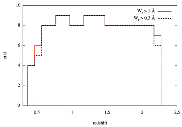
Figure 1: Redshift path density $g(z)$ of the UVES sample for $W_{\rm r}>0.3$ Å (black dashed line) and $W_{\rm r}>1.0$ Å  (red line).

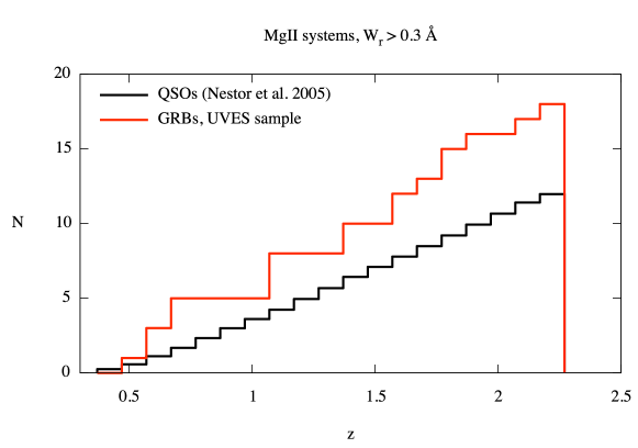
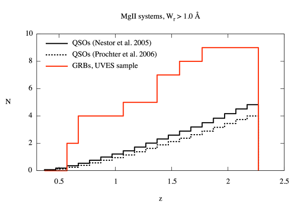
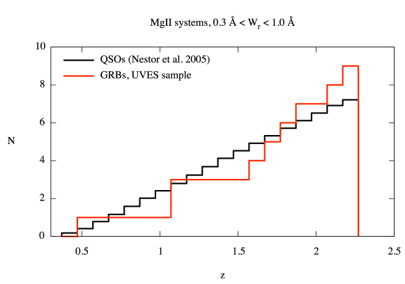
Figure 2: Comparison between the cumulative distribution of Mg ii systems detected along the UVES GRB los (red) and the one expected along QSO los following Eq. 2 (black solid) or Eq. 3 (black dashed), for: all (top panel), strong (middle panel) and weak (bottom panel) systems.

In Table 3 we also report the number of Mg ii absorbers that would be expected along lines of sight toward QSOs over the same redshift path, $N^{\rm MgII}_{\rm exp}$. To calculate these numbers, we determine the redshift path density, $g(z)$, of the UVES GRB sample (see Fig. 1) and combine it with the density of QSO absorbers per unit redshift as observed by Nestor et al. (2005) and Prochter et al. (2006a) (for the strong systems only) in the SDSS survey:

$$N^{\rm MgII}_{\rm exp}=\int_{z_{\rm start}}^{z_{\rm end}}\!g(z)\frac{\partial n}{\partial z}\,dz.$$ (2)

Both Nestor et al. (2005) and Prochter et al. (2006a) showed that the traditional parametrization of $\partial n/\partial z$ as a simple powerlaw $n_{0}(1+z)^{\gamma}$ does not provide a good fit to the SDSS data. Therefore we will use their empirical fits to the redshift number density. Nestor et al. (2005) give

$$\frac{\partial n}{\partial z}=\int\frac{dn}{dW_{\rm r}}(z)dW=\int\frac{n^{*}(z)}{W^{*}(z)}e^{-W_{r}/W^{*}}dW,$$ (3)

where both $n^{*}$ and $W^{*}$ vary with redshift as power laws: $n^{*}=1.001\pm 0.132(1+z)^{0.226\pm 0.170}$, $W^{*}=0.443\pm 0.032(1+z)^{0.634\pm 0.097}$. Prochter et al. (2006b) derive for the strong MgII systems:

$$\partial n/\partial z=-0.026+0.374z-0.145z^{2}+0.026z^{3}$$ (4)

The results of the calculations for the different $W_{\rm r}$ ranges ($W_{\rm r}>0.3$ Å , $W_{\rm r}>1.0$ Å  and $0.3\leq W_{\rm r}\leq 1.0$ Å) are shown in Fig. 2 and reported in Table 3. Errors are assumed to be poissonian and are scaled as $\sqrt{N^{\rm MgII}_{\rm exp}}$.

As a verification, we note from Fig. 13 of Nestor et al. (2005) that the number density, $\partial n/\partial z$, of $W_{\rm r}>0.3$ Å  systems is almost independent of the redshift. Multiplying the $\partial n/\partial z=0.783$ value reported there by the UVES ’all systems’ $\Delta z=13.79$ we obtain an expected total number of 9.78, in agreement with the value reported in Tab. 3 for systems along QSO los (i.e. 10.54). The same test performed using the number density values found by Steidel & Sargent (1992) give consistent results.

Fig. 2 and Table 3 show that the excess of strong Mg ii systems along GRB los compared to QSO los is significant at more than $2\sigma$ (slightly less than $2\sigma$ for the strong Mg ii systems if the Nestor et al. 2005 function is used), but it is more than a factor of $\sim 2$ lower than what is found by Prochter et al. (2006b). The number of weak systems is consistent within $\sim 1\sigma$ to that expected for QSO los.

3.2 The overall sample

Table 4: GRB los available from the literature.

GRB	$z_{\rm GRB}$	$z_{\rm start}$	$z_{\rm end}$	$z_{\rm abs}$	$W_{\rm r}(2796)$	$\Delta v_{\rm ej}$	Reference †
					(Å)	(km/s)
991216	1.022	0.366	1.002	0.770a	$4.0\pm 0.8^{b}$	$\sim 40000$	3
				0.803	$6.1\pm 0.7^{b}$	$\sim 34000$
000926	2.038	0.616	2.008				1
010222	1.477	0.430	1.452	0.927	$1.00\pm 0.14$	$\sim 74000$	2
				1.156	$2.49\pm 0.08$	$\sim 41000$
011211	2.142	0.366	1.932				3
020405	0.695	0.366	0.678	0.472	$1.1\pm 0.3$	$\sim 42000$	4
020813	1.255	0.366	1.232	1.224	$1.67\pm 0.02$	$\sim 4000$	5
030226	1.986	0.366	1.956				6
030323	3.372	0.824	1.646				7
030328	1.522	0.366	1.497				14
030429	2.66	0.620	1.861	0.8418	$3.3\pm 0.4^{b}$	$\sim 179000$	15
050505	4.275	1.414	2.27	1.695	$1.98$	$\sim 176000$	8
				2.265	$1.74$	$\sim 134000$
050908	3.35	0.814	2.27	1.548	$1.336\pm 0.107$	$\sim 147000$	9
051111	1.55	0.488	1.524	1.190	$1.599\pm 0.007$	$\sim 45000$	9,13
060206	4.048	1.210	2.27	2.26	$1.60$	$\sim 123000$	10
060526	3.221	0.836	2.27				11
071003	1.604	0.366	1.578	0.372	$2.48\pm 0.20$	$\sim 170000$	12

^† 1: Castro et al. (2003); 2: Mirabal et al. (2002); 3: Vreeswijk et al. (2006); 5: Barth et al. (2003); 4: Masetti et al. (2003);
6: Klose et al. (2004); 7: Vreeswijk et al. (2004); 8: Berger et al. (2006); 9: Prochter et al. (2006b); 10: Chen et al. (2008);
11: Thöne et al. (2008); 12: Perley et al. (2008); 13: Hao et al. (2007); 14: Maiorano et al. (2006); 15: Jakobsson et al. (2004).

^aThe very low resolution of the GRB 991216 spectrum makes the $z$=0.77 absorber identification uncertain. ^bThe $W_{\rm r}$ values refer to the total equivalent width of the MgII doublet.

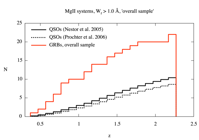
Figure 3: Comparison between the cumulative distribution of strong Mg ii systems in the overall sample of GRB los (red) and the one expected along QSO los following Eq. 2 (black solid) or Eq. 3 (black dashed).

In order to increase the statistics of strong Mg ii systems, we added to the UVES sample both high and low resolution GRB afterglow spectra published in the literature. The resulting sample is composed of 26 los (see Table 4 for details on los that are not part of the UVES sample). Since this sample includes many low resolution spectra, we study the statistics of strong ($W_{\rm r}$ $>$ 1 Å) Mg ii absorbers only, using the same redshift limits as in the previous Section. Three lines of sight of this sample (GRB 991216, GRB 000926 and GRB 030429) were not used by Prochter et al. (2006b) because the low spectral resolution of these spectra does not allow to resolve the Mg ii doublet. However, such a low resolution does not prevent the detection of strong systems, although the doublet is blended. In addition, the total equivalent width of the doublets detected along these los is larger than 3 Å so that we are confident that $W_{\rm r,2796}$ is larger than 1 Å. In any case, as detection of Mg ii systems is more difficult at lower resolution, including these lines of sight could only underestimate their number density.

The total number of strong Mg ii systems is $N=22$ and the redshift path is $\Delta z=31.55$. This leads to a number density $\partial n/\partial z=0.70\pm 0.15$. We use the $g(z)$ function of this enlarged sample to compute the total number of strong systems expected for a similar QSO sample following the same method as used in Sect. 3.1. We find $N^{\rm MgII}_{\rm exp}=10.41\pm 3.23$ and $N^{\rm MgII}_{\rm exp}=8.62\pm 2.94$, using Eq. 3 and 4, respectively, that is $2.1\pm 0.6$ and $2.6\pm 0.8$ times less than the number found along GRB los (see Fig. 3).

The excess of strong Mg ii systems along GRB lines of sight for this enlarged sample is confirmed at a $\sim 3\sigma$ statistical significance. The excess found is higher than for the UVES sample but still a factor of $\sim 2$ lower than what was previously reported by Prochter et al. (2006b) from a sample with a smaller redshift path. The number densities resulting from the two studies are different by no more than 2$\sigma$. For consistency we also performed our analysis considering only the smaller sample used by Prochter et al. (2006b). In this case, the results obtained are similar to those found by these authors. The redshift path of our overall sample is twice as large as that used by Prochter et al. (2006b), therefore the factor of 2 excess we find in this study has a higher statistical significance.

3.3 Number density evolution

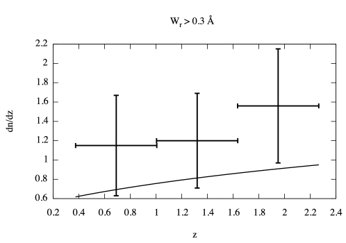
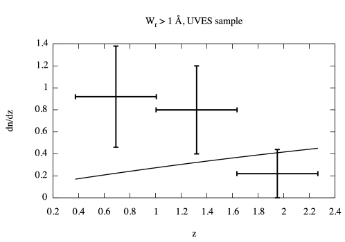
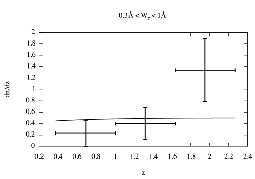
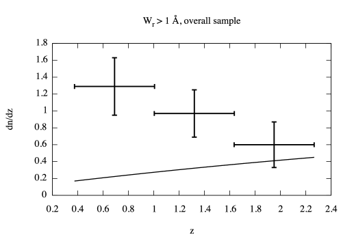
Figure 4: Number density evolution of Mg ii systems detected along GRB los for: first panel: all, second panel: strong, third panel: weak systems of the UVES sample; bottom panel: strong systems of the overall sample. The solid line represents the evolution of the MgII number density derived from the Mg ii survey in the SDSS QSO by Nestor et al. (2005) (see Eq. 3).

We divided both the UVES and the overall sample in three redshift bins and calculated $\partial n/\partial z$ for each bin. Fig. 4 shows the number of systems per redshift bin. While the total number of systems and the number of weak systems have a comparable redshift evolution in GRB and QSO lines of sight, the strong systems happen to have a different evolution in GRB los. The excess of strong systems in GRBs is particularly pronounced at low redshift, up to $z\sim 1.6$. We performed a KS test for each of the three cases to assess the similarity of the redshift distribution of Mg ii systems along GRB and QSO los. There is a $90.7\%$ and $23.5\%$ chance that the weak and all Mg ii absorber samples in QSOs and GRBs are drawn from the same population. The probability for the strong systems is $20.1\%$ for the UVES sample, but it decreases to $\sim 2\%$ when considering the overall sample.

This apparent excess of strong systems in the low-redshift bin could indicate that some amplification bias due to lensing is at work. Indeed the effect of lensing should be larger in case the deflecting mass is at smaller redshift. The lensing optical depth for GRBs at redshift $z_{\rm GRB}>>1$ and $z_{\rm GRB}\leq 1$ is maximal for a lens at respectively $z_{\rm l}\sim 0.7$ and $z_{\rm GRB}/2$. However, we find that only 47% of GRBs with strong foreground absorbers in our sample have at least one strong Mg ii system located in the range within which the optical depth decreases to about half its maximum value (Sudilovsky et al. 2007; Turner 1980; Smette et al. 1997). This indicates that if amplification by lensing is the correct explanation, the effect must be weak and subtle. Porciani et al. (2007) used the optical afterglow luminosities reported by Nardini et al. (2006) to show that GRB afterglows with more than one absorbers are brigther than others by a factor 1.7. However this correlation has not been detected by Sudilovsky et al. (2007) when using the afterglow B-band absolute magnitudes obtained by Kann et al. (2006, 2007).

More data and larger samples are obviously needed to conclude on this issue.

4 The population of strong Mg ii systems

Both the results on the UVES homogeneous sample and those obtained using the overall sample confirm, although to a smaller extent, the excess of strong Mg ii absorbers along GRB los first reported by Prochter et al. (2006b). To understand the reason of the discrepancy in the number density of “strong” systems it is therefore important to study in more details these systems and to derive their physical characteristics. This is possible using the UVES data. The main question we would like to address here is whether there is any reason to believe that GRB and QSO strong absorbers are not drawn from the same population.

4.1 Equivalent width distribution

We show in Fig. 5 the comparison between the normalized $W_{\rm r}$ distribution of all Mg ii systems with $W_{\rm r}$ $>$ 0.3 Å  detected in the UVES sample and the one reported by Nestor et al. (2005) for the Mg ii systems along the QSO los in the SDSS survey.

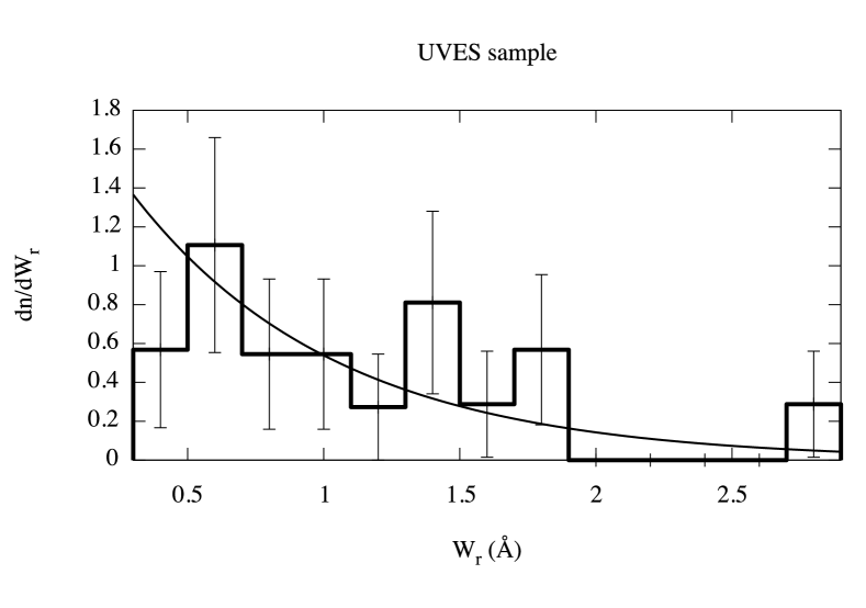
Figure 5: $W_{\rm r}$ distribution of the Mg ii systems with $W_{\rm r}$ $>$ 0.3 Å  detected in the UVES sample. The solid curve represents the corresponding distribution for QSO MgII absorbers (Nestor et al. 2005). Both distributions have been normalized such that their underlying areas are equal to 1.

The KS tests give a $27.1\%$ chance that the GRB and QSO distributions are drawn from the same population for the UVES sample. This result extends to lower $W_{\rm r}$ values the conclusion by Porciani et al. (2007) that the two distributions are similar, arguing against the idea that the excess of Mg ii systems could be related to the internal structure of the intervening clouds.

4.2 The velocity spread of strong Mg ii systems

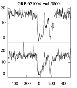
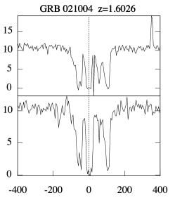
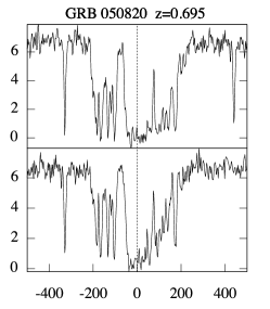
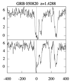
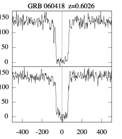
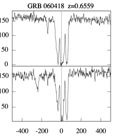
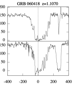
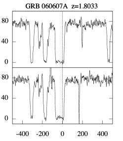
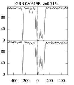
Figure 6: The $W_{\rm r}>1.0$ Å Mg ii absorption systems detected in the UVES spectra. the Mg ii $\lambda$2796 (top) and $\lambda$2803 (bottom) absorption lines are displayed for each system on a relative velocity scale with 0 km s^-1 centered at the redshift reported in Table 1.

The profiles of the two transitions of the $W_{\rm r}$ $>$ 1 Å  Mg ii systems found in the UVES spectra are plotted on a velocity scale in Fig. 6. The profiles are complex, spread over at least 200 km s^-1 and up to $\sim 600$ km s^-1 and show a highly clumpy structure.

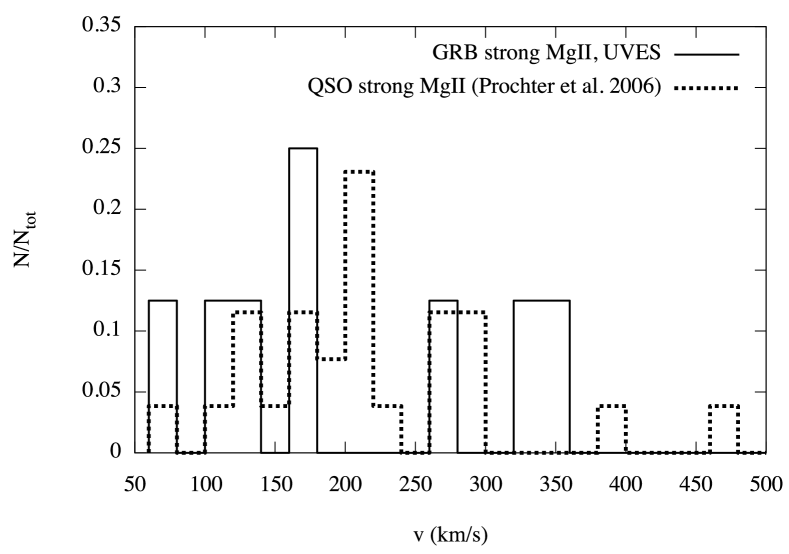
Figure 7: The solid line histogram represents the distribution of the velocities of the strong Mg ii systems in the UVES sample calculated following Ledoux et al. (2006). The thick dashed histogram refers to the 27 SDSS Mg ii systems observed at high spectral resolution (Prochter et al. 2006a).

We measure the velocity spread of the Mg ii systems with $W_{\rm r}$ $>$ 1.0 Å in the UVES sample following Ledoux et al. (2006). We therefore use a moderately saturated low ionization absorption line (e.g. FeII${\lambda 2344}$, SiII${\lambda 1526}$) and measure the velocity difference between the points of the absorption profiles at which 5% and 95% of the absorption occurs. This method is defined in order to measure the velocity width of the bulk of gas, avoiding contamination by satellite components which have negligible contribution to the total metal column density. Note that using this definition implies that the measured velocity spread is usually smaller than the spread of the Mg ii profile which is strongly saturated. In case no moderately saturated absorption line is available, we use the mean value of the velocity widths calculated both from a saturated line and an optically thin line. Results are given in column 9 of Table 6.

The velocity-spread distribution is shown for UVES systems with $W_{\rm r}$ $>$ 1 Å  in Fig. 7 together with the SDSS QSO distribution from 27 SDSS systems with $W_{\rm r}$ $>$ 1 Å  observed at high spectral resolution (Prochter et al. 2006a). Although the statistics are small, the UVES and SDSS distributions are statistically similar. A KS test gives 65% chance that the two samples are drawn from the same population (see also Cucchiara et al. 2008).

4.3 Dust extinction

It has been proposed that a dust bias could possibly affect the statistics of strong Mg ii systems. Indeed, if part of the population of strong Mg ii systems contains a substantial amount of dust, then the corresponding lines of sight could be missed in QSO surveys because of the attenuation of the quasar whereas GRBs being intrinsically brighter, the same lines of sight are not missed when observing GRBs. The existence of a dust extinction bias in DLA surveys is still a debated topic among the QSO community although observations of radio selected QSO los (Ellison et al. 2004) seem to show that, if any, this effect is probably small (see also Pontzen & Pettini 2008).

Table 5: Iron to Zinc or Silicon ratio and extinction estimate for 4 strong Mg ii systems.

	$z$	$N$(FeII)	$N$(ZnII)	$N$(SiII)	[Fe/Zn]	[Fe/Si]	$N_{\rm Fe}^{\rm dust}$	$A_{\rm V}$
		(cm-2)	(cm-2)	(cm-2)			(cm-2)
GRB021004	1.3800	$15.09\pm 0.05$		$15.19\pm 0.09$		$-0.05\pm 0.10$	$14.18\pm 0.23$	$\sim 0$
GRB021004	1.6026	$14.60\pm 0.03$	$12.78\pm 0.02$		$-1.03\pm 0.04$		$15.59\pm 0.02$	$<0.2$
GRB060418	1.1070	$14.69\pm 0.01$	$12.87\pm 0.03$		$-1.05\pm 0.03$		$15.68\pm 0.03$	$<0.2$
GRB060607A	1.8033	$14.07\pm 0.03$		$14.36\pm 0.10$		$-0.24\pm 0.10$	$13.94\pm 0.17$	$\sim 0$

We can use our UVES lines of sight to estimate the dust content of strong Mg ii systems from the depletion of iron compared to other non-depleted species as is usually done in DLAs. We have therefore searched for both Fe ii and Zn ii absorption lines (or Si ii, in case the Zn ii lines are not available) associated to the strongest Mg ii systems present in the UVES spectra. Because the spectra do not always cover the relevant wavelength range, the associated column densities could be measured only for 4 out of the 10 systems (see Table 5). We estimate the depletion factor, and therefore the presence of dust, from the metallicity ratio of iron (a species heavily depleted into dust grains in the ISM of our Galaxy) to zinc (that is little depleted), [Fe/Zn] = (Fe/Zn)$-$(Fe/Zn)_☉ (or [Fe/Si]). We also determine the iron dust phase column density ($N_{\rm Fe}^{\rm dust}$) using the formula given by Vladilo et al. (2006) and from this we infer an upper limit on the corresponding flux attenuation $A_{\rm V}$ from their Fig. 4. We used also the estimate given by (Bohlin et al. 1978; Prochaska & Wolfe 2002):

$$A_{\rm V}=0.5\frac{N({\rm HI})}{10^{21}}\kappa=0.5\frac{10^{\rm X}}{10^{21}\times 10^{\rm[X/H]_{\sun}}}(1-10^{\rm[Fe/X]})$$ (5)

with $\kappa=10^{\rm[X/H]}(1-10^{\rm[Fe/X]})$ representing the dust-to-gas ratio and X corresponding to Zn or Si if Zn is not available.

Results are reported in Table 5. It can be seen that although depletion of iron can be significant, the corresponding attenuation is modest because the column densities of metallic species are relatively small owing to low metallicities (see also Table 5). Indeed we find high dust depletion in two systems at $z_{\rm abs}$ = 1.107 toward GRB 060418 (see also Ellison et al. 2006) and at $z_{\rm abs}$ = 1.6026 toward GRB 021004. Their column densities are low however so that the inferred $A_{\rm V}$ does not exceed values typically found for QSO los (see Vladilo et al. 2006 and Prantzos & Boissier 2000). Cucchiara et al. (2008) do not detect the Zn II absorption lines for the systems at $z_{\rm abs}$ = 1.6026 toward GRB 021004. They report an upper limit of $W_{\rm r}<0.016$ Å  whereas we find $W_{\rm r}=0.07$ Å. The detection of Zn II($\lambda$$\lambda$2026,2062) for the central component seems robust, as it is shown in Fig. 8. In addition, the Cr II($\lambda$$\lambda$2056,2062) lines are also possibly detected.

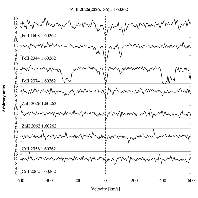
Figure 8: Fe II($\lambda$$\lambda$1608,2344,2374), Zn II($\lambda$$\lambda$2026,2062) and Cr II($\lambda$$\lambda$2056,2062) transition lines at $z_{\rm abs}$ = 1.6026 in the spectra of the afterglow of GRB 021004, shown in velocity space. The dashed line correspond to $z_{\rm abs}$ = 1.6026. The Zn II absorption lines are clearly detected for the central component of the system.

We note that for GRB 021004 and GRB 060607A we could estimate the attenuation for ALL strong Mg ii systems identified along the los. Therefore our results do not show evidences to support the idea that a bias due to the presence of dust in strong Mg ii systems could be an explanation for the overabundance of the strong Mg ii absorbers along GRB los. On the other hand, the fact that 2 out of 4 of the selected systems have a dust depletion higher than the values usually found for QSO DLAs (Meiring et al. 2006) supports the fact that these systems probably arise in the central part of massive halos where the probability to find cold gas is expected to be higher.

5 Estimating the H i column density

Table 6: Characteristics of Mg ii systems with $W_{\rm r}>1.0$ Å  in the UVES sample.

GRB	$z_{\rm abs}$	$W_{\rm r}^{MgII\lambda 2796}$	$W_{\rm r}^{MgI\lambda 2852}$	$W_{\rm r}^{FeII\lambda 2600}$	$N_{\rm ZnII}$	$N_{\rm SiII}$	$N_{\rm FeII}$	${}^{a}\Delta v$	${}^{b}\Delta v^{MgII\lambda 2796}$
		(Å)	(Å)	(Å)	cm-2	cm-2	cm-2	km s-1	km s-1
021004	1.380	1.637	0.190	0.972		$15.19\pm 0.09$	$15.09\pm 0.05$	170	89
021004	1.603	1.407	0.366	0.737	$12.78\pm 0.02$		$14.60\pm 0.03$	164	51
050820A	0.692	2.874	$N/A^{c}$	$N/A^{c}$			$N/A^{c}$		228
050820A	1.429	1.323	0.488	0.601			$14.34\pm 0.03$	271	98
060418	0.603	1.293	0.361	0.989			$16.43\pm 0.04^{d}$	76	130
060418	0.656	1.033	0.078	0.486			$13.96\pm 0.02$	136	123
060418	1.107	1.844	0.483	1.080	$12.87\pm 0.03$		$14.69\pm 0.01$	119	221
060607A	1.803	1.854	$>0.226$	0.825		$14.36\pm 0.1$	$14.07\pm 0.03$	333	90
080319B	0.715	1.482	0.303	0.697			$14.00\pm 0.01$	354	142

^a Velocities are measured following Ledoux et al. (2006); ^b Velocities are measured using the MgII$\lambda 2796$ absorption considering only the central part of the system, following the method recommended by Ellison et al. (2009); ^c Lines redshifted on top of the Ly${-\alpha}$ absorption associated to the GRB or in the Ly${-\alpha}$ forest; ^d Saturated line.

A key parameter to characterize an absorber is the corresponding H i column density. Unfortunately, the H i Lyman-$\alpha$ absorption line of most of the systems is located below the atmospheric cut-off and is unobservable from the ground. If we want to characterize the systems with their H i column density or at least an estimate of it, we have to infer it indirectly. For this we will assume that the strong systems seen in front of GRBs and QSOs are cosmological and drawn from the same population. We believe that the results discussed in the previous section justify this assumption.

We use the velocity-metallicity correlation found by Ledoux et al. (2006) to estimate the expected metallicity of the systems in the UVES sample with $W_{\rm r}$ $>$ 1.0 Å, assuming that the correlation is valid also for sub-DLA systems (Péroux et al. 2008). The relation was linearly extrapolated to the average redshift of the sample of systems with $W_{\rm r}$ $>$ 1.0 Å , $\langle z\rangle=1.11$, giving [X/H]$=1.43{\rm log}\Delta v-3.78$. We infer the hydrogen column densities dividing the zinc, silicon or iron column densities measured in the UVES spectrum by the metallicity. Note that in most of the cases only Fe ii available (see Table 5). The $N$(H i) column density derived in these cases should be considered a lower limit because iron can be depleted onto dust-grains. The results are shown in Table 7 (columns 3 and 4). The error on the procedure should be of the order of 0.5 dex (see Ledoux et al. 2006). We insist on the fact that our aim is not to derive an exact H i column density for each system but rather to estimate the overall nature of the systems. We find that at least 3 of the 9 systems with $W_{\rm r}$ $>$ 1 Å  could be DLAs. In any case, and even if we consider that we systematically overestimate the column density by 0.5 dex, a large fraction of the systems should have log $N$(H i) $>$ 19.

Another method to infer the presence of DLAs among Mg ii absorbers is to use the ‘D-index’ (Ellison et al. 2009). We calculate the D-index for the systems in our sample following the recommended D-index definition by Ellison et al. (2009) and using the formula:

$$D=\frac{W_{\rm r}({\rm MgII}\lambda 2796)({\rm\AA})}{\Delta v({\rm MgII}\lambda 2796)({\rm km/s})}\times\frac{{\rm log}N({\rm FeII})}{15}\times 1000.$$ (6)

The width of the central part of the Mg ii$\lambda 2796$ absorption system, $\Delta v$(MgII$\lambda$2796) in km/s, is reported in column 10 of Table 6 while the resulting D-index values are reported in Table 7 (column 5). Note that if we do not include the iron column density term in the D-index calculation, we obtain similar results.

We find that all the 9 systems have $D>7$. Ellison et al. (2009) find that $57^{+18.3}_{-14.0}\%$ of the systems having $D>7$ are DLAs. This results applied to our sample imply that at least 5 systems are DLAs. We can compare the number of DLAs per unit redshift ($n_{\rm DLA}$) found for the QSO los by Rao et al. (2006) to that of our GRB sample. $n_{\rm DLA}$ is defined as the product of the Mg ii systems number density and the fraction of DLAs in a Mg ii sample. Rao et al. (2006) found $n_{\rm DLA,QSO}\sim 0.1$ (with errors of the order of 0.02). If we assume that three to five systems in our sample are DLAs we find $n_{\rm DLA,GRB}\sim 0.22-0.36$ . This means that the number of DLAs is at least two times larger along GRB lines of sight as compared to QSO lines of sight.

The above estimate of log $N$(H i) can be considered as highly uncertain and the identification of a few of the systems as DLAs can be questioned.

All this seems to indicate that GRBs favor lines of sight with an excess of DLAs. Since these systems are more likely to be located in the central parts of massive halos, this may again favor the idea that there exists a bias in GRB observations towards GRBs with afterglows brighter because they are subject to some lensing amplification.

Table 7: Inferred metallicity, $N_{\rm HI}$ and $D$-index of Mg ii systems with $W_{\rm r}>1.0$ Å  in the UVES sample.

GRB	$z_{\rm abs}$	[X/H]a	$N_{\rm HI}({\rm cm}^{-2})^{b}$	$D$-indexc
021004	1.380	$-0.63$	20.3	$8.32\pm 0.22$
021004	1.603	$-0.65$	20.8	$9.99\pm 0.47$
050820A	0.692			$9.0\pm 0.03^{d}$
050820A	1.429	$-0.34$	$>19.2$	$8.13\pm 0.22$
060418	0.603	$-1.13$	$>22.0$	$10.39\pm 0.09^{e}$
060418	0.656	$-0.77$	$>19.2$	$7.51\pm 0.05$
060418	1.107	$-0.85$	21.1	$8.17\pm 0.06$
060607A	1.803	$-0.21$	19.0	$9.12\pm 0.06$
080319B	0.715	$-0.17$	$>18.7$	$8.06\pm 0.01$

^a Metallicities inferred using the velocity-metallicity relation found by Ledoux et al. (2006); ^b $N_{\rm HI}$ values inferred using the velocity-metallicity relation found by Ledoux et al. (2006). When only the iron column density is available, the $N_{\rm HI}$ value has to be considered has a lower limit due to possible dust extinction; ^c D-index calculated using Eq. 6, following the method recommended by Ellison et al. (2009); ^d D-index calculated without including the iron column density term (see Ellison et al. 2009); ^e iron lines are saturated. The D-index calculated without including the iron column density term would be $D=9.48\pm 0.08$;

6 Observed sub-DLA absorbers

The UVES spectra often cover a substantial part of the Lyman-$\alpha$ forest in front of the GRB. It is therefore possible to search directly for strong H i Lyman-$\alpha$ absorption lines corresponding to DLAs or, more generally, sub-DLAs. This can only be performed for 8 of the 10 GRBs in the sample: the redshifts of GRB 060418 and GRB 080319B are unfortunately too low to allow the detection of the Lyman-$\alpha$ absorptions in the UVES spectral range. We exclude from our search the DLA at the GRB redshift, which is believed to be associated with the close surrounding of the GRB. We find additional (sub-)DLAs (Fig. 9) along the los of GRB 050730 (see also Chen et al. 2005), GRB 050820, GRB 050922C (see also Piranomonte et al. 2008) and GRB 060607A (Fig. 10). The former three systems are simple, with a single Lyman-$\alpha$ component. The system detected at 2.9374 toward GRB 060607A is more complex and cannot be fit with a single component (sub-) DLA. The profile is made of two main clumps at $z=2.9322$ and 2.9374. The latter is a blend of the four O i components (see top panel in Fig. 9). The constraints on the H i column densities come mostly from the red wing of the Lyman-$\alpha$ line and the structures seen in the Lyman-$\gamma$ line. We find that the two main H i components at $z=2.9374$ and 2.9322 have log $N$(H i) $=\leavevmode\nobreak\ 19.4$ and $19.0\pm 0.1$, respectively. It is worth noting that the limit on the O i component at $z=2.9322$ is log $N$(O i) $<12.6$ implying that the metallicity in the cloud could be as low as [O/H] $<$ $-2.9$ which would be the lowest metallicity ever observed yet in such a system. Some ionization correction could be necessary however in case the oxygen equilibrium is displaced toward high excitation species by a hard ionizing spectrum.

Table 8 shows the column densities and abundances of the systems assuming that all elements are in their neutral or singly ionized state. The values are similar to those usually found for (sub)-DLAs along QSO los (see for example Péroux et al. 2003).

The presence of these systems allows us to extend the search for strong systems along GRB lines of sight to higher redshift. The redshift paths (see Table 8) have been calculated considering $z_{\rm start}$ as the redshift of an absorber, for which the corresponding Lyman-$\alpha$ line would be redshifted to the same wavelength as the Lyman-$\beta$ line of the GRB afterglow. We therefore avoid confusion with the Lyman-$\beta$ forest. $z_{\rm end}$ is fixed at 3000 km/s from the GRB redshift. The only exception to this rule is GRB 050730 for which there is a gap in the spectrum located at about 3000 km/s from the GRB redshift and starting at $\lambda=5096$ Å. We use this wavelength to fix $z_{\rm max}$. The corresponding total redshift path is $\Delta z=4.17$. The sub-DLAs systems at $z=2.9322$ and 2.9374 along GRB 060607A are separated by $\sim$400 km s^-1, therefore for the statistical study we consider them as a single system. The resulting number density for systems with log $N$(H i)$>$19.0 is $0.96\pm 0.48$ for an average redshift of $\langle z\rangle=2.08$. At this redshift a value of about $0.5\pm 0.2$ is expected from QSO los (Péroux et al. 2005). There could be therefore an excess of such systems but the statistics is obviously poor.

It is intriguing however that the four systems we detect are all in the half of the Lyman-$\alpha$ forest closest to the GRB, with ejection velocities of about 25000, 22000, 12000 and 11000 km s^-1 for GRB 050730, 050820A, 050922C and 060607A respectively. The corresponding ejection velocities found for the strong Mg ii systems (see column 7 of Table 2) are larger than 35000 km/s, making an origin local to the GRB unlikely for the strong Mg ii systems. This fact therefore does not favor the possibility that the excess of strong Mg ii absorbers along GRB los is due to some ejected material present in the GRB environment. The much lower ejection velocities found for the sub-DLA absorbers may indicate that for these systems the excess is not of the same origin as the excess of Mg ii systems and that part of the gas in these systems could have been ejected by the GRB.

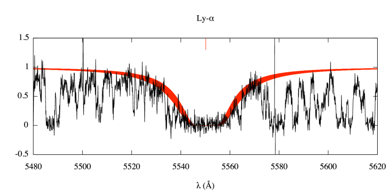
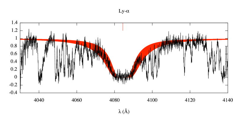
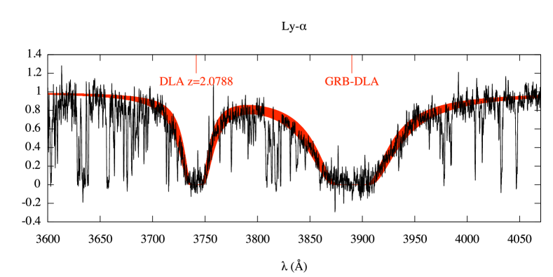
Figure 9: Foreground (sub)-DLAs. Top panel: Sub-damped Lyman-$\alpha$ absorption at $z=3.5655$ toward GRB 050730. Middle panel: Damped Lyman-$\alpha$ absorption at $z=2.3598$ toward GRB 050820. Bottom panel: Sub-damped Lyman-$\alpha$ absorption at $z=2.0778$ toward GRB 050922C (this system has been fitted together with the DLA associated to the GRB at $z=2.1999$). The red area correspond to the fit result covering the column density error range.

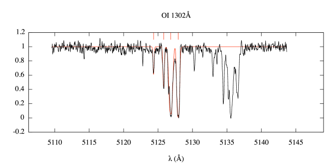
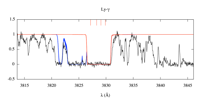
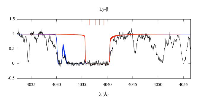
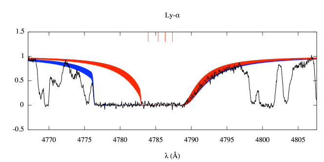
Figure 10: The sub-DLA system at $z=2.9374$ along the los toward GRB 060607A. The top panel shows the fit of the O i$\lambda$1302 absorption profile, while the following panels report the fit results of the Lyman-$\gamma$, Lyman-$\beta$ and Lyman-$\alpha$ absorption lines (from top to bottom, respectively). The red lines show the main $z=2.9374$ component (different lines include errors) mostly constrained by the red wing of the Lyman-$\alpha$ absorption. In blue is shown the total fit including the sub-DLA component at $z=2.9322$.

7 Conclusion

We have taken advantage of UVES observations of GRB afterglows obtained over the past six years to build an homogeneous sample of lines of sight observed at high spectral resolution and good signal-to-noise ratio (SNR$>$10). We used these observations to re-investigate the claimed excess of Mg ii systems along GRB lines of sight extending the study to smaller equivalent widths. We also used these data to derive intrinsic physical properties of these systems.

Considering the redshift ranges $0.37<z<2.27$ of the SDSS survey used for the QSO statistics, we find an excess of strong intervening MgII systems along the 10 GRB lines of sight observed by UVES of a factor of $\sim 2$ compared to QSO lines of sigth. This excess is significant at $\sim 2\sigma$. Thanks to the quality of the UVES data it has been possible also to consider the statistics of the weak absorbers (0.3 $<$ $W_{\rm r}$ $<$ 1.0 Å). We find that the number of weak absorbers is similar along GRBs and QSOs lines of sight.

Table 8: Properties of the foreground damped Ly-$\alpha$ systems detected along the UVES GRB spectra.

	$\Delta z$a	z	log $N_{\rm{}_{HI}}$	log $N_{\rm OI}$	log $N_{\rm SiII}$	log $N_{\rm FeII}$	[Fe/Si]	[O/H]	[Si/H]	[Fe/H]
		(Sub-)DLA	($N$ in cm-2)	($N$ in cm-2)	($N$ in cm-2)	($N$ in cm-2)
GRB021004	0.487	There are no intervening (Sub-)DLA along this los
GRB050730	0.542	3.5655	$20.2\pm 0.1$	$N/A^{b}$	$<14.7$	$<13.6$			$<-1.0$	$<-2.3$
GRB050820A	0.529	2.3598	$20.1\pm 0.2$	$N/A^{b}$	$13.84\pm 0.02$	$14.11\pm 0.02$	$-0.22\pm 0.02$		$-1.5\pm 0.2$	$-1.7\pm 0.2$
GRB050922C	0.468	2.0778	$20.65\pm 0.15$	$>15.30$	$14.38\pm 0.10$	$14.44\pm 0.03$	$0.11\pm 0.10$	$>-2.1$	$-1.83\pm 0.18$	$-1.72\pm 0.15$
GRB060607A	0.596	$2.9374^{c}$	$19.4\pm 0.1$	$>15.07$	$>14.74^{d}$	$14.16\pm 0.03$	$<-0.53$	$>-1.1$	$>-0.2$	$-0.7\pm 0.1$
		$2.9322^{c}$	$19.0\pm 0.1$	$<12.8$	$<12.6$	$<12.6$		$<-2.9$	$<-1.9$	$<-1.9$
GRB071031	0.540	There are no intervening (Sub-)DLA along this los
GRB080310	0.501	There are no intervening (Sub-)DLA along this los
GRB080413A	0.503	There are no intervening (Sub-)DLA along this los

^a Redshift path calculated from the Ly-$\beta$ GRB absorption line to 3000 km/s from the GRB Ly-$\alpha$, except for GRB 050730 where the $z$ range ends at the beginning of the spectral gap at $\lambda=5096$Å. ^b The line is blended with other lines in the Ly-$\alpha$ forest. ^c To calculate the DLA number density we counted the $z=2.9374$ and $z=2.9322$ systems as a single system.
^d Blended with the Si iv$\lambda$1402 absorption line associated to the GRB.

We increase the absorption length for strong systems to $\Delta z$ = 31.5 using intermediate and low resolution observations reported in the literature. The excess of strong MgII intervening systems of a factor of $\sim 2$ is confirmed at $3\sigma$ significance. We therefore strenghten the evidence that the number of strong sytems is larger along GRB lines of sight, even if this excess is less than what has been claimed in previous studies based on a smaller path length (see Prochter et al. 2006b). Our result and that of Prochter et al. (2006b) are different at less than $2\sigma$. The present result is statistically more significant.

Possible explanations of this excess include: dust obscuration that could yield such lines of sight to be missed in quasar studies; difference of the beam sizes of the two types of background sources; gravitational lensing. In order to retrieve more information to test these hypotheses we investigate in detail the properties of the strong Mg ii systems observed with UVES. We find that the equivalent width distribution of Mg ii systems is similar in GRBs and QSOs. This suggests that the absorbers are more extended than the beam size of the sources which should not be the case for the different beam sizes to play a role in explaining the excess (Porciani et al. 2007). In addition, we divide our sample in three redshift bins and we find that the number density of strong Mg ii systems is larger in the low redshift bins, favoring the idea that current sample of GRB lines of sight can be biased by gravitational lensing effect. We also estimate the dust extinction associated to the strong GRB Mg ii systems and we find that it is consistent with what is observed in standard (sub)-DLAs. It therefore seems that the dust-bias explanation has little grounds.

We tentatively infer the H i column densities of the strong systems and we note that the number density of DLAs per unit redshift in the UVES sample is probably twice larger than what is expected from QSO sightlines. As these sytems are expected to arise from the central part of massive haloes, this further supports the idea of a gravitational lensing amplification bias. This hypothesis could be also supported by the results recently obtained by (Chen et al. 2008). These authors analyzed 7 GRB fields and found the presence of at least one addition object at angular separation from the GRB afterglow position in all the four fields of GRBs with known intervening strong MgII galaxies. In contrast, none is seen at this small angular separation in fields without known Mg II absorbers.

We searched the Lyman-$\alpha$ forest probed by the UVES spectra for the presence of damped Lyman-$\alpha$ absorption lines. We found four sub-DLAs with log $N$(H i) $>$ 19.3 over a redshift range of $z=4.3$. This is again twice larger than what is expected in QSOs. However the statistics is poor. It is intriguing that these systems are all located in the half redshift range of the Lyman-$\alpha$ forest closest to the GRB. It is therefore not excluded that part of this gas is somehow associated with the GRBs. In that case, ejection velocities of the order of 10 to 25 000 km/s are required.