Geometric integrators for multiplicative viscoplasticity: analysis of error accumulation

Abstract

The inelastic incompressibility is a typical feature of metal plasticity/viscoplasticity. Over the last decade, there has been a great amount of research related to construction of numerical integration algorithms which exactly preserve this geometric property. In this paper we examine, both numerically and mathematically, the excellent accuracy and convergence characteristics of such geometric integrators.

In terms of a classical model of finite viscoplasticity, we illustrate the notion of exponential stability of the exact solution. We show that this property enables the construction of effective and stable numerical algorithms, if incompressibility is exactly satisfied. On the other hand, if the incompressibility constraint is violated, spurious degrees of freedom are introduced. This results in the loss of the exponential stability and a dramatic deterioration of convergence behavior.

,

AMS Subject Classification: 74C20; 65L20.

Nomenclature

$\mathbf{C}_{\text{i}}$	inelastic right Cauchy-Green tensor (see (25))
$\tilde{\mathbf{T}}$	2nd Piola-Kirchhoff tensor (see (27))
$\mathbf{1}$	second-rank identity tensor
$\mathbf{A}\cdot\mathbf{B}=\mathbf{A}\mathbf{B}$	product (composition) of two second-rank tensors
$\mathbf{A}:\mathbf{B}$	scalar product of two second-rank tensors
$\mathbf{A}\otimes\mathbf{B}$	tensor product of two second-rank tensors
$\|\mathbf{A}\|$	$l_{2}$ norm of a second-rank tensor (Frobenius norm)
$\|\mathbf{A}\|^{*}$	induced norm of a second-rank tensor (spectral norm) (see (1))
$(\cdot)^{\text{D}}$	deviatoric part of a tensor
$(\cdot)^{\text{T}}$	transposition of a tensor
$(\cdot)^{-\text{T}}$	inverse of transposed
$\text{tr}(\cdot)$	trace of a second-rank tensor
$\overline{(\cdot)}$	unimodular part of a tensor (see (2))
$\text{sym}(\cdot)$	symmetric part of a tensor
$\langle x\rangle$	MacCauley bracket (see $(\ref{examp3})_{3}$)
$\psi_{\text{el}}$	specific free energy density
$\text{Dist}(\cdot,\cdot)$	”distance” between two solutions (see (39))
$K$	yield stress
$\lambda_{\text{i}}$	proportionality factor (inelastic multiplier) (see $(\ref{prob3})_{1}$)
$f$	overstress (see $(\ref{prob3})_{2}$)
$\mathfrak{F}$	norm of the driving force (see $(\ref{prob3})_{3}$)
$Sym$	space of symmetric second-rank tensors
$M$	invariant manifold (cf. (5), (30))
$\rho_{\scriptscriptstyle\text{R}}$	mass density in the reference configuration
$k$	bulk modulus (see (33))
$\mu$	shear modulus (see (33))

1 Introduction

The mechanical processing of materials may involve very large inelastic deformations. For instance, for equal channel angular extrusion of aluminum alloys, the introduced accumulated inelastic strain usually varies between 100 and 900 Percent (depending on the number of extrusions [34]). Even larger deformations can be introduced by some incremental forming procedures like spin extrusion [21] (the accumulated inelastic strain ranges up to 1000 Percent). Due to the highly nonlinear character of the underlying mechanical problem, a correct numerical simulation of such ”long” processes is by no means a trivial task. It is desirable to have numerical algorithms which would be stable with respect to numerical errors, even if working with big time intervals and big time steps.

The assumption of exact inelastic incompressibility is widely implemented for construction of material models of metal plasticity and creep (see, for instance, [11]). Extensive studies were carried out concerning the construction of numerical integration algorithms which exactly preserve the incompressibility of the inelastic flow [4, 10, 13, 20, 23, 27, 30, 31].

In this paper, we asses those factors that result in a more accurate computations, especially when integrating with big time steps and for long times. To this end, we analyze the structural properties of the inelastic flow governed by a classical material model of finite viscoplasticity. The material model is based on the multiplicative decomposition of the deformation gradient into inelastic and elastic parts. For simplicity, no hardening behavior is considered in this paper. However, the proposed methodology can be generalized to cover more complicated material behavior as well.

We pay especial attention to the exponential stability of the inelastic flow, which is the key notion of the current study. We say that the solution to a Cauchy problem is exponentially stable, if for small perturbations of initial data, an exponential decay estimate holds (see Section 2.1). From mechanical standpoint, the exponential stability implies fading memory behavior. Moreover, the exponential stability is deeply connected to contractivity (B-stability) of the system of equations, which can be used for stability analysis of numerical algorithms (see the monograph by Simo and Hughes [29]).

The main conclusions of this paper regarding the problem of finite viscoplasticity are as follows.

• The exact solution is exponentially stable with respect to small perturbations of initial data, if the incompressibility constraint is not violated.

• In the case of exponential stability, the numerical error is uniformly bounded. In particular, there is no error accumulation even within large time periods.

• If the incompressibility constraint is violated by some numerical algorithm, then, in general, the numerical error tends to accumulate over time.

There exists a rich mathematical literature dealing with existence, uniqueness, regularity, and asymptotic behavior of solutions for certain plascticity/viscoplasticity problems in the context of infinitesimal strains (see [1, 8, 14] and references therein). A class of material models of monotone type which includes the class of generalized standard materials was defined and analyzed in [1]. In the context of finite viscoplasticity, however, only few theoretical works exist. Some preliminary investigations have been made by Neff in [24].

In this paper, we analyze the well-known material model of finite viscoplasticity. The stability is proved analogously to the classical Lyapunov approach, based on the use of Lyapunov-candidate-functions. In fact, the hyperelastic potential is used to construct a suitable Lyapunov candidate (cf. [29]).

The paper is organized as follows. In Section 2, we define the notion of exponential stability and prove the main theorem, which states that the numerical error is uniformly bounded if the exact solution is exponentially stable. A simple one-dimensional example is presented. In the next section, a classical material model of finite viscoplasticity is formulated in the reference configuration. The change of the reference configuration is likewise discussed. Section 4 contains the definition and analysis of the distance between two solutions in terms of energy (Lyapunov candidate). Next, the time-evolution of the distance is evaluated and the exponential stability of the exact solution is proved. Finally, the results of numerical tests are presented, which illustrate the excellent accuracy and convergence characteristics of geometric integrators.

We conclude this introduction with a few words regarding notation. Expression $a:=b$ means $a$ is defined to be another name for $b$. Throughout this article, bold-faced symbols denote first- and second-rank tensors in $\mathbb{R}^{3}$. A coordinate-free tensor setting is used in this paper (cf. [15, 28]). The scalar product of two second rank tensors is defined by $\mathbf{A}:\mathbf{B}=\text{tr}(\mathbf{A}\mathbf{B}^{\text{T}})$. This scalar product gives rise to the norm by $\|\mathbf{A}\|:=\sqrt{\mathbf{A}:\mathbf{A}}$. Moreover, we denote by $\|\cdot\|^{*}$ the induced norm of a tensor

$$\|\mathbf{A}\|^{*}:=\max_{\|\mathbf{x}\|_{2}=1}\|\mathbf{A}\mathbf{x}\|_{2},\quad\|\mathbf{x}\|_{2}:=\sqrt{\mathbf{x}\cdot\mathbf{x}}.$$ (1)

The overline $\overline{(\cdot)}$ stands for the unimodular part of a tensor

$$\overline{\mathbf{A}}:=(\det\mathbf{A})^{-1/3}\mathbf{A}.$$ (2)

The deviatoric part of a tensor is defined as $\mathbf{A}^{\text{D}}:=\mathbf{A}-\frac{1}{3}\text{tr}(\mathbf{A})\mathbf{1}$. The notation $O$ stands for ”Big-O” Landau symbol: $f(x)=O(g(x))\ \text{as}\ x\ \rightarrow x_{0}$ iff there exists $C<\infty\ \text{such that}\ \|f(x)\|\leq C\|g(x)\|\ \text{as}\ x\ \rightarrow x_{0}$. The inequality $f(x)\leq O(g(x))$ is understood as follows: there exists $\acute{f}(x)=O(g(x))$ such that $f(x)\leq\acute{f}(x)$.

2 Differential equations on manifolds and exponential stability

2.1 General definitions

Let us consider the Cauchy problem for a smooth function $y(t)\in\mathbb{R}^{n}$

$${}\dot{y}(t)=f(y(t),d(t)),\quad y(t_{0})=y_{0}.$$ (3)

Here, the initial value $y_{0}$ and the function $d(t)$ are supposed to be given. Denote the exact solution to (3) by $\tilde{y}(t,y_{0},t_{0})$. In particular, we have

$${}\tilde{y}(t_{0},y_{0},t_{0})=y_{0}.$$ (4)

Suppose that all solutions lie on some manifold $M\subset\mathbb{R}^{n}$

$${}\tilde{y}(t,y_{0},t_{0})\in M,\quad\text{for all}\ t\geq t_{0},\ y_{0}\in M.$$ (5)

Then we say that (3) is a differential equation on the manifold $M$ (cf. [6, 7]).

Next, we say that the solution $y(t)$ to the problem (3) is locally exponentially stable on $M$, if there exist $\delta>0,\ \gamma>0,\ C_{1}<\infty$, such that the following decay estimate holds

$${}\|\tilde{y}(t,y^{(1)}_{0},t_{0})-\tilde{y}(t,y^{(2)}_{0},t_{0})\|\leq C_{1}\ \e^{\displaystyle-\gamma(t-t_{0})}\ \|y^{(1)}_{0}-y^{(2)}_{0}\|,$$ (6)

for all $t_{0}\geq 0$, $y^{(1)}_{0},y^{(2)}_{0}\in M$ such that $\|y^{(1)}_{0}-y(t_{0})\|\leq\delta$, $\|y^{(2)}_{0}-y(t_{0})\|\leq\delta$.

We note that somewhat different interpretation of the exponential stability can be met in the literature as well (cf., for example, Section 2.5 of [16]).

Next, let us consider a numerical algorithm which solves (3) on the time interval $[0,T]$. Denote by ${}^{n}y$ the numerical solutions at time instances ${}^{n}t$, where $0={}^{0}t<{}^{1}t<{}^{2}t<...<{}^{N}t=T$, and ${}^{0}y=y_{0}$. Suppose that the error on the step is bounded by the second power of the step size. More precisely

$${}\|\tilde{y}({}^{n+1}t,{}^{n}y,{}^{n}t)-{}^{n+1}y\|\leq C_{2}({}^{n+1}t-{}^{n}t)^{2},$$ (7)

where $C_{2}<\infty$ (cf. figure 1). For simplicity, we will consider constant time-steps only: $\Delta t={}^{n+1}t-{}^{n}t=const$.

2.2 Main theorem

With definitions from previous section we formulate the following theorem.

Theorem 1.

Let $y(t)=\tilde{y}(t,y_{0},0)$ be the exact solution. Suppose that conditions (6) and (7) hold. Moreover, suppose that the numerical solution of problem (3) lies exactly on $M$. Then there exist a constant $C<\infty$ such that

$${}\|{}^{n}y-y({}^{n}t)\|\leq C\Delta t,\quad\text{as}\ \Delta t\rightarrow 0.$$ (8)

Here, the constant $C$ does not depend on the size of the time interval $[0,T]$.

Proof. The proof is a modification of the standard error analysis (cf. [2]). In this paper we prove the theorem under assumption that $\delta=\infty$. The proof can be easily generalized to cover arbitrary values of $\delta>0$ by using mathematical induction and by assuming $\Delta t\leq\gamma\delta/(2\max({C_{1},1})\ C_{2})$.

First, note that $\tilde{y}({}^{n}t,{}^{0}y,{}^{0}t)=y({}^{n}t)$. Thus, (cf. figure 1)

$${}\|{}^{n}y-y({}^{n}t)\|\leq\|{}^{n}y-\tilde{y}({}^{n}t,{}^{n-1}y,{}^{n-1}t)\|+\|\tilde{y}({}^{n}t,{}^{n-1}y,{}^{n-1}t)-\tilde{y}({}^{n}t,{}^{n-2}y,{}^{n-2}t)\|+...\\ +\|\tilde{y}({}^{n}t,{}^{1}y,{}^{1}t)-\tilde{y}({}^{n}t,{}^{0}y,{}^{0}t)\|.$$ (9)

\psfrag{A0}[m][1][0]{${}^{0}t$}\psfrag{A1}[m][1][0]{${}^{1}t$}\psfrag{A2}[m][1][0]{${}^{2}t$}\psfrag{A3}[m][1][0]{${}^{3}t$}\psfrag{A4}[m][1][0]{${}^{4}t$}\psfrag{B}[m][1][0]{${}^{4}y$}\psfrag{C}[m][1][0]{$\tilde{y}({}^{4}t,{}^{3}y,{}^{3}t)$}\psfrag{D}[m][1][0]{$\tilde{y}({}^{4}t,{}^{2}y,{}^{2}t)$}\psfrag{E}[m][1][0]{$\tilde{y}({}^{4}t,{}^{1}y,{}^{1}t)$}\psfrag{F}[m][1][0]{$y({}^{4}t)$}\psfrag{G}[m][1][0]{Exact solution}\psfrag{H}[m][1][0]{Numerical solution}\includegraphics{fig1.eps}

Figure 1: Analysis of error accumulation.

Next, from (6) we obtain for all $k=1,2,...,n-1$

$${}\|\tilde{y}({}^{n}t,{}^{k}y,{}^{k}t)-\tilde{y}({}^{n}t,{}^{k-1}y,{}^{k-1}t)\|\leq C_{1}\ \e^{\displaystyle-\gamma({}^{n}t-{}^{k}t)}\ \|\tilde{y}({}^{k}t,{}^{k}y,{}^{k}t)-\tilde{y}({}^{k}t,{}^{k-1}y,{}^{k-1}t)\|.$$ (10)

Substituting (10) in (9), we get

$${}\|{}^{n}y-y({}^{n}t)\|\leq\\ \|{}^{n}y-\tilde{y}({}^{n}t,{}^{n-1}y,{}^{n-1}t)\|+C_{1}\sum_{k=1}^{n-1}\e^{\displaystyle-\gamma({}^{n}t-{}^{k}t)}\ \|\tilde{y}({}^{k}t,{}^{k}y,{}^{k}t)-\tilde{y}({}^{k}t,{}^{k-1}y,{}^{k-1}t)\|.$$ (11)

Obviously, $\tilde{y}({}^{k}t,{}^{k}y,{}^{k}t)={}^{k}y$. Without loss of generality, we can assume that $C_{1}\geq 1$. Next, substituting error estimation (7) into (11), we get

$${}\|{}^{n}y-y({}^{n}t)\|\leq C_{1}\ C_{2}\ (\Delta t)^{2}\sum_{k=1}^{n}\e^{\displaystyle-\gamma({}^{n}t-{}^{k}t)}.$$ (12)

But, ${}^{n}t-{}^{k}t=(n-k)\Delta t$. Thus, taking into account the well-known expression for an infinite geometric series ($\sum_{i=0}^{\infty}r^{i}=1/(1-r)$ for $|r|<1$ ), we get for small $\Delta t$

$${}\sum_{k=1}^{n}\e^{\displaystyle-\gamma({}^{n}t-{}^{k}t)}\leq\sum_{i=0}^{\infty}\e^{\displaystyle-i\gamma\Delta t}=\frac{\displaystyle 1}{\displaystyle 1-\e^{-\gamma\Delta t}}=\frac{\displaystyle 1}{\displaystyle\gamma\Delta t+O((\Delta t)^{2})}\leq 2\frac{\displaystyle 1}{\displaystyle\gamma\Delta t}.$$ (13)

Finally, it follows from (12), (13)

$${}\|{}^{n}y-y({}^{n}t)\|\leq\frac{\displaystyle 2C_{1}\ C_{2}}{\displaystyle\gamma}\ \Delta t,\quad\text{as}\ \Delta t\rightarrow 0\quad\quad\quad\quad\quad\quad\blacksquare$$ (14)

Remark 1. The proof is essentially based on the assumption that ${}^{k}y\in M$. In general, if the numerical solution ${}^{k}y$ leaves the manifold $M$, the decay estimation (6) is not valid.

Remark 2. The theorem states that the error is uniformly bounded in the case of exponential stability. Thus, there is no error accumulation in the sense that the constant $C$ in (8) does not depend on the overall time $T$. Moreover, let $\epsilon>0$ be some small value. By choosing $\Delta t\leq\gamma\epsilon/(2C_{1}C_{2})$ the numerical error $\|{}^{n}y-y({}^{n}t)\|$ is guaranteed to be less than $\epsilon$.

Remark 3. If the exponential stability is replaced by the assumption that the right-hand side of (3) is a smooth function of $y$, a weaker error estimation is valid (cf. [2])

$${}\|{}^{n}y-y({}^{n}t)\|\leq C\e^{LT}T\ \Delta t,\quad\text{as}\ \Delta t\rightarrow 0,$$ (15)

where $L=\sup\|f_{y}\|$. The effect of growing multiplier on the right hand side of (15) is referenced to as an effect of error accumulation. In that case, in order to guaranty a sufficient accuracy, the upper bound for $\Delta t$ must depend on $T$. That makes the practical solution of some problems extremely expensive for large values of $T$.

2.3 One-dimensional example

Let us consider a simple example which illustrates the notion of exponential stability. We examine the response of a one-dimensional viscoplastic device shown in Figure 2 (a).

\psfrag{A}[m][1][0]{$\varepsilon_{\text{i}}$}\psfrag{B}[m][1][0]{$\varepsilon_{\text{e}}$}\psfrag{C}[m][1][0]{$\varepsilon$}\psfrag{B1}[m][1][0]{$\varepsilon_{\text{i}}$}\psfrag{A1}[m][1][0]{$t$}\psfrag{E}[m][1][0]{(a)}\psfrag{F}[m][1][0]{(b)}\includegraphics{fig2.eps}

Figure 2: Rheological model (a), and inelastic flow under monotonic loading (b).

The closed system of (constitutive) equations is as follows:

The total strain is decomposed into elastic part $\varepsilon_{\text{e}}$, and inelastic part $\varepsilon_{\text{i}}$

$${}\varepsilon=\varepsilon_{\text{e}}+\varepsilon_{\text{i}}.$$ (16)

The stress $\sigma$ on the elastic spring is governed by elasticity law ($E>0$).

$${}\sigma=E\varepsilon_{\text{e}}.$$ (17)

The time derivative of the inelastic strain is given by

$${}\dot{\varepsilon}_{\text{i}}=\frac{1}{\eta}\langle f\rangle\frac{\sigma}{|\sigma|},\quad f:=|\sigma|-K,\quad\langle x\rangle:=\max(x,0),$$ (18)

where material constants $K>0$ and $\eta>0$ are referred to as yield stress and viscosity, respectively.

In order to use the results of previous subsections, we rewrite the problem in the form

$${}\dot{\varepsilon}_{\text{i}}=\dot{\varepsilon}_{\text{i}}(\varepsilon_{\text{i}},\varepsilon(t))=\frac{1}{\eta}\langle E|\varepsilon(t)-\varepsilon_{\text{i}}|-K\rangle\ \text{sign}(\varepsilon(t)-\varepsilon_{\text{i}}).$$ (19)

Let $\varepsilon^{(1)}_{\text{i}}(t)$ and $\varepsilon^{(2)}_{\text{i}}(t)$ be to two solutions to (19). Following [29], we recall that
$\sqrt{\frac{1}{2}E(\varepsilon^{(1)}_{\text{i}}-\varepsilon^{(2)}_{\text{i}})^{2}}$ defines an energy norm which is the natural norm for the problem under consideration. Next, we consider a monotonic loading

$${}\varepsilon(t)=\dot{\varepsilon}t,\quad\dot{\varepsilon}=const>0.$$ (20)

Let us show that the exact solution satisfying the initial condition $\varepsilon_{\text{i}}=0$ is exponentially stable. Without loss of generality, we can assume that $t_{0}=0$ in estimation (6). If $|\varepsilon^{(k)}_{\text{i}}(0)-0|\leq\delta$ for $\text{k}\in\{1,2\}$, then there exists time instance $t^{\prime}=t^{\prime}(\delta)$ such that the condition $f\geq f_{0}>0$ holds for both solutions ($\varepsilon^{(1)}_{\text{i}}(t)$ and $\varepsilon^{(2)}_{\text{i}}(t)$), if $t\geq t^{\prime}$ (see Figure 2 (b)). Then, under that assumption

$${}\frac{\partial\dot{\varepsilon}_{\text{i}}(\varepsilon_{\text{i}},\varepsilon(t))}{\partial\varepsilon_{\text{i}}}=-\frac{E}{\eta},\quad\dot{\varepsilon}_{\text{i}}(\varepsilon^{(1)}_{\text{i}},\varepsilon(t))-\dot{\varepsilon}_{\text{i}}(\varepsilon^{(2)}_{\text{i}},\varepsilon(t))=-\frac{E}{\eta}(\varepsilon^{(1)}_{\text{i}}-\varepsilon^{(2)}_{\text{i}}).$$ (21)

Therefore, we get from (21)

$${}\Big{(}\frac{1}{2}E(\varepsilon^{(1)}_{\text{i}}-\varepsilon^{(2)}_{\text{i}})^{2}\Big{)}^{\cdot}=E(\varepsilon^{(1)}_{\text{i}}-\varepsilon^{(2)}_{\text{i}})(\dot{\varepsilon}^{(1)}_{\text{i}}-\dot{\varepsilon}^{(2)}_{\text{i}})=-\frac{E^{2}}{\eta}(\varepsilon^{(1)}_{\text{i}}-\varepsilon^{(2)}_{\text{i}})^{2},\ \text{for}\ t\geq t^{\prime}.$$ (22)

Due to the contractivity (for details see [29]), $\frac{1}{2}E(\varepsilon^{(1)}_{\text{i}}(t^{\prime})-\varepsilon^{(2)}_{\text{i}}(t^{\prime}))^{2}\leq\frac{1}{2}E(\varepsilon^{(1)}_{\text{i}}(0)-\varepsilon^{(2)}_{\text{i}}(0))^{2}$. Moreover, integrating (22) over $[t^{\prime},t]$ and taking the contractivity into account, we get

$${}\frac{1}{2}E(\varepsilon^{(1)}_{\text{i}}(t)-\varepsilon^{(2)}_{\text{i}}(t))^{2}\leq\frac{1}{2}E(\varepsilon^{(1)}_{\text{i}}(0)-\varepsilon^{(2)}_{\text{i}}(0))^{2}\e^{-\frac{2E}{\eta}(t-t^{\prime})}.$$ (23)

Taking the square root of both sides we obtain the required exponential decay estimation (6) with $C_{1}=\e^{\frac{\displaystyle Et^{\prime}}{\displaystyle\eta}}<\infty$ and $\gamma=\frac{\displaystyle E}{\displaystyle\eta}>0$.

3 Material model of multiplicative viscoplasticity

Let us consider a classical material model of finite viscoplasticity (see, for example, [11]).

3.1 Constitutive equations

The model is based on the multiplicative split of the deformation gradient $\mathbf{F}$

$$\mathbf{F}=\hat{\mathbf{F}}_{\text{e}}\mathbf{F}_{\text{i}}.$$ (24)

Here, $\hat{\mathbf{F}}_{\text{e}}$ and $\mathbf{F}_{\text{i}}$ stand for elastic and inelastic parts, respectively (see [17, 18]). The multiplicative split can be motivated by the idea of a local elastic unloading. A somewhat more consistent motivation can be derived from the concept of material isomorphism [3].

Along with the well-known right Cauchy-Green tensor ${\mathbf{C}}=\mathbf{F}^{\text{T}}\mathbf{F}$, we introduce a strain-like internal variable (inelastic right Cauchy-Green tensor) as

$${\mathbf{C}}_{\text{i}}=\mathbf{F}^{\text{T}}_{\text{i}}\mathbf{F}_{\text{i}}.$$ (25)

In this paper we consider strain-driven processes. More precisely, we assume the deformation history ${\mathbf{C}}(t)$ to be given. The material response in the time interval $t\in[0,T]$ is governed by the following ordinary differential equation with initial condition

$$\dot{\mathbf{C}}_{\text{i}}=2\frac{\displaystyle\lambda_{\text{i}}}{\displaystyle\mathfrak{F}}\big{(}\mathbf{C}\tilde{\mathbf{T}}\big{)}^{\text{D}}\mathbf{C}_{\text{i}},\quad\mathbf{C}_{\text{i}}|_{t=0}=\mathbf{C}_{\text{i}}^{0},\ \det\mathbf{C}_{\text{i}}^{0}=1,\ \mathbf{C}_{\text{i}}^{0}\in Sym.$$ (26)

Here, the 2nd Piola-Kirchhoff tensor $\tilde{\mathbf{T}}$, the norm of the driving force $\mathfrak{F}$, and the inelastic multiplier $\lambda_{\text{i}}$ are functions of $(\mathbf{C},\mathbf{C}_{\text{i}})$, given by

$$\tilde{\mathbf{T}}=2\rho_{\scriptscriptstyle\text{R}}\frac{\displaystyle\partial\psi_{\text{el}}(\mathbf{C}{\mathbf{C}_{\text{i}}}^{-1})}{\displaystyle\partial\mathbf{C}}\big{|}_{\mathbf{C}_{\text{i}}=\text{const}},$$ (27)

$$\lambda_{\text{i}}=\frac{\displaystyle 1}{\displaystyle\eta}\Big{\langle}\frac{\displaystyle 1}{\displaystyle k_{0}}f\Big{\rangle}^{m},\quad f:=\mathfrak{F}-\sqrt{\frac{2}{3}}K,\quad\mathfrak{F}:=\sqrt{\text{tr}\big{[}\big{(}\mathbf{C}\tilde{\mathbf{T}}\big{)}^{\text{D}}\big{]}^{2}}.$$ (28)

The material parameters $\rho_{\scriptscriptstyle\text{R}}>0$, $\eta\geq 0$, $m\geq 1$, $K>0$, and the isotropic real-valued function $\psi_{\text{el}}$ are assumed to be known; $k_{0}>0$ is used to get a dimensionless term in the bracket.

Remark. The right Cauchy strain tensor $\mathbf{C}$ is symmetric. Since the function $\psi_{\text{el}}$ is isotropic, it makes no difference whether the derivative in (27) is understood as a general derivative or as a derivatives with respect to a symmetric tensor (cf. [28]).

Next, we remark that the right-hand side in $\eqref{prob1}_{1}$ is symmetric (cf. [28]). Moreover, taking into account the property $\text{tr}(\mathbf{A}\mathbf{B})=\text{tr}(\mathbf{B}\mathbf{A})$ and combining the Jacobi formulae $\frac{\displaystyle\partial\text{det}(\mathbf{A})}{\displaystyle\partial\mathbf{A}}=\text{det}(\mathbf{A})\ \mathbf{A}^{-\text{T}}$ with the evolution equation $\eqref{prob1}_{1}$, we get

$$\big{(}\det\mathbf{C}_{\text{i}}\big{)}^{\cdot}=\frac{\displaystyle\partial\text{det}(\mathbf{\mathbf{C}_{\text{i}}})}{\displaystyle\partial\mathbf{\mathbf{C}_{\text{i}}}}:\dot{\mathbf{C}}_{\text{i}}=2\frac{\displaystyle\lambda_{\text{i}}}{\displaystyle\mathfrak{F}}\text{det}(\mathbf{\mathbf{C}_{\text{i}}})\ \mathbf{C}_{\text{i}}^{-1}:\big{(}\mathbf{C}\tilde{\mathbf{T}}\big{)}^{\text{D}}\mathbf{C}_{\text{i}}=2\frac{\displaystyle\lambda_{\text{i}}}{\displaystyle\mathfrak{F}}\text{tr}\big{[}\big{(}\mathbf{C}\tilde{\mathbf{T}}\big{)}^{\text{D}}\big{]}=0.$$ (29)

Therefore, the exact solution of (26) – (28) has the following geometric property

$$\mathbf{C}_{\text{i}}\in M,\quad M:=\big{\{}\mathbf{B}\in Sym\ |\ \text{det}\mathbf{B}=1\big{\}}.$$ (30)

We note that the current material model is thermodynamically consistent. That means that the Clausius-Duhem inequality holds for arbitrary mechanical loadings

$$\delta_{\text{i}}:=\frac{1}{2\rho_{\scriptscriptstyle\text{R}}}\tilde{\mathbf{T}}:\dot{\mathbf{C}}-\big{(}\psi_{\text{el}}(\mathbf{C}{\mathbf{C}_{\text{i}}}^{-1})\big{)}^{\cdot}\geq 0.$$ (31)

In particular, we get a reduced inequality for relaxation processes ($\mathbf{C}=\text{const}$)

$$\big{(}\psi_{\text{el}}(\mathbf{C}{\mathbf{C}_{\text{i}}}^{-1})\big{)}^{\cdot}\ \leq 0.$$ (32)

One mathematical interpretation of this inequality will be discussed in Section 4.1.

To be definite, we use the following expression for the free energy density $\psi_{\text{el}}$ (generalized Neo-Hooke model [11])

$$\rho_{\scriptscriptstyle\text{R}}\psi_{\text{el}}(\mathbf{A}):=\frac{k}{2}\big{(}\text{ln}\sqrt{\text{det}\mathbf{A}}\big{)}^{2}+\frac{\mu}{2}\big{(}\text{tr}\overline{\mathbf{A}}-3\big{)},$$ (33)

where $k>0$, $\mu>0$ are known material constants (bulk modulus and shear modulus, respectively).

Substituting (33) in (27) we get the 2nd Piola-Kirchhoff stress tensor in the form

$$\tilde{\mathbf{T}}=k\ \text{ln}\sqrt{\text{det}(\mathbf{C})}\ \mathbf{C}^{-1}+\mu\ \mathbf{C}^{-1}(\overline{\mathbf{C}}\mathbf{C}_{\text{i}}^{-1})^{\text{D}}.$$ (34)

In what follows we analyze the exponential stability of the exact solution $\mathbf{C}_{\text{i}}(t)$.

3.2 Change of reference configuration

In order to simplify the analysis of the material model, we may need to rewrite the constitutive equation with respect to some ”new” local reference configuration $\mathbf{F}_{0}$. In what follows, we suppose that this configuration is isochoric, i.e. $\det(\mathbf{F}_{0})=1$. The ”new” deformation gradient, right Cauchy tensor, and inelastic right Caushy tensor are given by

$$\mathbf{F}^{\text{new}}:=\mathbf{F}\mathbf{F}^{-1}_{0},\quad\mathbf{C}^{\text{new}}:=\mathbf{F}^{-\text{T}}_{0}\mathbf{C}\mathbf{F}^{-1}_{0},\quad\mathbf{C}^{\text{new}}_{\text{i}}:=\mathbf{F}^{-\text{T}}_{0}\mathbf{C}_{\text{i}}\mathbf{F}^{-1}_{0}.$$ (35)

The 2nd Piola-Kirchhoff tensor $\tilde{\mathbf{T}}$, the norm of the driving force $\mathfrak{F}$, the inelastic multiplier $\lambda_{\text{i}}$, and the overstress $f$ are transformed as follows

$$\tilde{\mathbf{T}}^{\text{new}}:=\mathbf{F}_{0}\tilde{\mathbf{T}}\mathbf{F}^{\text{T}}_{0},\quad\mathfrak{F}^{\text{new}}:=\mathfrak{F},\quad\lambda_{\text{i}}^{\text{new}}:=\lambda_{\text{i}}\quad f^{\text{new}}:=f.$$ (36)

Since $\psi_{\text{el}}$ is isotropic, $\psi_{\text{el}}(\mathbf{A}\mathbf{B})=\psi_{\text{el}}(\mathbf{B}\mathbf{A})$. Using that property, it can be checked that $\psi_{\text{el}}(\mathbf{C}{\mathbf{C}_{\text{i}}}^{-1})$ is invariant under the change of reference configuration

$$\psi_{\text{el}}(\mathbf{C}^{\text{new}}(\mathbf{C}^{\text{new}}_{\text{i}})^{-1})=\psi_{\text{el}}(\mathbf{C}{\mathbf{C}_{\text{i}}}^{-1}).$$ (37)

The closed system of equations with respect to the new reference configuration is obtained from (26) — (28) by replacing all quantities by their ”new” counterparts.

4 Analysis of exponential stability for multiplicative viscoplasticity

4.1 Measuring the distance between solutions in terms of energy

Suppose that $\mathbf{C}^{(1)}_{\text{i}}(t)$ and $\mathbf{C}^{(2)}_{\text{i}}(t)$ are two solutions to the problem (26) — (28) (with the same forcing function $\mathbf{C}(t)$). Next, suppose that there exists a constant $L<\infty$ such that

$$\|(\mathbf{C}^{(k)}_{\text{i}})^{1/2}(t)\|<L,\quad\|(\mathbf{C}^{(k)}_{\text{i}})^{-1/2}(t)\|<L\quad\text{for all}\ t>0,\ k\in\{1,2\}.$$ (38)

We introduce the following measure of distance between two solutions in terms of energy

$$\text{Dist}(\mathbf{C}^{(1)}_{\text{i}},\mathbf{C}^{(2)}_{\text{i}}):=\sqrt{\rho_{\scriptscriptstyle\text{R}}\psi_{\text{el}}\big{(}\mathbf{C}^{(1)}_{\text{i}}(\mathbf{C}^{(2)}_{\text{i}})^{-1}\big{)}}.$$ (39)

This measure has the following properties:

(i) Invariance under the change of reference configuration

$$\text{Dist}\big{(}(\mathbf{C}^{(1)}_{\text{i}})^{\text{new}},(\mathbf{C}^{(2)}_{\text{i}})^{\text{new}}\big{)}=\text{Dist}\big{(}\mathbf{C}^{(1)}_{\text{i}},\mathbf{C}^{(2)}_{\text{i}}\big{)}.$$ (40)

(ii) For small $\mathbf{C}^{(1)}_{\text{i}}-\mathbf{C}^{(2)}_{\text{i}}$, there exist constants $C_{3}>0$ and $C_{4}<\infty$ such that

$$C_{3}\ \|\mathbf{C}^{(1)}_{\text{i}}-\mathbf{C}^{(2)}_{\text{i}}\|\leq\text{Dist}(\mathbf{C}^{(1)}_{\text{i}},\mathbf{C}^{(2)}_{\text{i}})\leq C_{4}\|\mathbf{C}^{(1)}_{\text{i}}-\mathbf{C}^{(2)}_{\text{i}}\|.$$ (41)

(iii) For all $\mathbf{C}^{(1)}_{\text{i}}(t),\mathbf{C}^{(2)}_{\text{i}}(t)\in M$ we have $\text{Dist}(\mathbf{C}^{(1)}_{\text{i}},\mathbf{C}^{(2)}_{\text{i}})\geq 0$ and

$$\text{Dist}(\mathbf{C}^{(1)}_{\text{i}},\mathbf{C}^{(2)}_{\text{i}})=0,\ \text{if and only if}\ \ \mathbf{C}^{(1)}_{\text{i}}=\mathbf{C}^{(2)}_{\text{i}}.$$ (42)

Proof.

(i): Identity (40) can be proved similarly to the invariance property (37).

(ii): First, it follows from (33) that for small $\mathbf{\Delta}$ we have (see Appendix A)

$$\rho_{\scriptscriptstyle\text{R}}\psi_{\text{el}}(\mathbf{1}+\mathbf{\Delta})=\frac{k}{8}(\text{tr}\mathbf{\Delta})^{2}+\frac{\mu}{4}\text{tr}\big{(}(\mathbf{\Delta}^{\text{D}})^{2}\big{)}+O(\Delta^{3}),$$ (43)

where $\Delta=\|\mathbf{\Delta}\|$. Note that $\text{tr}\big{(}(\mathbf{\Delta}^{\text{D}})^{2}\big{)}=\|\mathbf{\Delta}^{\text{D}}\|^{2}$ for $\mathbf{\Delta}\in Sym$. Thus, $\frac{k}{8}(\text{tr}\mathbf{\Delta})^{2}+\frac{\mu}{4}\text{tr}\big{(}(\mathbf{\Delta}^{\text{D}})^{2}\big{)}$ is a norm on $Sym$. Since all norms on $Sym$ are equivalent, there exist constants $C^{\prime}_{3}>0$, $C^{\prime}_{4}<\infty$ such that for small $\mathbf{\Delta}\in Sym$ we have

$$C^{\prime}_{3}\|\mathbf{\Delta}\|^{2}\leq\rho_{\scriptscriptstyle\text{R}}\psi_{\text{el}}(\mathbf{1}+\mathbf{\Delta})\leq C^{\prime}_{4}\|\mathbf{\Delta}\|^{2}.$$ (44)

Next, due to the property

$$\psi_{\text{el}}(\mathbf{A}\mathbf{B})=\psi_{\text{el}}(\mathbf{B}\mathbf{A}),$$ (45)

we have

$$\text{Dist}(\mathbf{C}^{(1)}_{\text{i}},\mathbf{C}^{(2)}_{\text{i}})=\sqrt{\rho_{\scriptscriptstyle\text{R}}\psi_{\text{el}}\big{(}(\mathbf{C}^{(2)}_{\text{i}})^{-1/2}\ \mathbf{C}^{(1)}_{\text{i}}\ (\mathbf{C}^{(2)}_{\text{i}})^{-1/2}\big{)}}.$$ (46)

Moreover, taking into account that $\|\mathbf{A}\mathbf{B}\|_{*}\leq\|\mathbf{A}\|_{*}\ \|\mathbf{B}\|_{*}$, and that the norms $\|\cdot\|_{*}$ and $\|\cdot\|$ are equivalent, we get

$$\|\mathbf{A}\mathbf{B}\mathbf{C}\|\leq\acute{C}\|\mathbf{A}\|\ \|\mathbf{B}\|\ \|\mathbf{C}\|,$$ (47)

with some constant $\acute{C}<\infty$. Thus,

$$\big{\|}(\mathbf{C}^{(2)}_{\text{i}})^{-1/2}\ \mathbf{C}^{(1)}_{\text{i}}\ (\mathbf{C}^{(2)}_{\text{i}})^{-1/2}-\mathbf{1}\big{\|}=\big{\|}(\mathbf{C}^{(2)}_{\text{i}})^{-1/2}\ \big{(}\mathbf{C}^{(1)}_{\text{i}}-\mathbf{C}^{(2)}_{\text{i}}\big{)}\ (\mathbf{C}^{(2)}_{\text{i}})^{-1/2}\big{\|}\\ \stackrel{{\scriptstyle\eqref{EnerDist8}}}{{\leq}}\acute{C}\big{\|}(\mathbf{C}^{(2)}_{\text{i}})^{-1/2}\big{\|}^{2}\ \big{\|}\mathbf{C}^{(1)}_{\text{i}}-\mathbf{C}^{(2)}_{\text{i}}\big{\|},$$ (48)

$$\big{\|}\mathbf{C}^{(1)}_{\text{i}}-\mathbf{C}^{(2)}_{\text{i}}\big{\|}=\big{\|}(\mathbf{C}^{(2)}_{\text{i}})^{1/2}\big{(}(\mathbf{C}^{(2)}_{\text{i}})^{-1/2}\ \mathbf{C}^{(1)}_{\text{i}}\ (\mathbf{C}^{(2)}_{\text{i}})^{-1/2}-\mathbf{1}\big{)}(\mathbf{C}^{(2)}_{\text{i}})^{1/2}\big{\|}\\ \stackrel{{\scriptstyle\eqref{EnerDist8}}}{{\leq}}\acute{C}\big{\|}(\mathbf{C}^{(2)}_{\text{i}})^{1/2}\big{\|}^{2}\ \big{\|}(\mathbf{C}^{(2)}_{\text{i}})^{-1/2}\ \mathbf{C}^{(1)}_{\text{i}}\ (\mathbf{C}^{(2)}_{\text{i}})^{-1/2}-\mathbf{1}\big{\|}.$$ (49)

Further, substituting $\mathbf{\Delta}=(\mathbf{C}^{(2)}_{\text{i}})^{-1/2}\ \mathbf{C}^{(1)}_{\text{i}}\ (\mathbf{C}^{(2)}_{\text{i}})^{-1/2}-\mathbf{1}$ in (44), and combining it with (46), (48), and (49) we get

$$\tilde{C}_{3}\|(\mathbf{C}^{(2)}_{\text{i}})^{1/2}\|^{-2}\ \|\mathbf{C}^{(1)}_{\text{i}}-\mathbf{C}^{(2)}_{\text{i}}\|\leq\text{Dist}(\mathbf{C}^{(1)}_{\text{i}},\mathbf{C}^{(2)}_{\text{i}})\leq\tilde{C}_{4}\|(\mathbf{C}^{(2)}_{\text{i}})^{-1/2}\|^{2}\ \|\mathbf{C}^{(1)}_{\text{i}}-\mathbf{C}^{(2)}_{\text{i}}\|.$$ (50)

Finally, combining (50) with (38) we obtain (41).

(iii): We note that $\psi_{\text{el}}(\mathbf{A})\geq 0$. Moreover, $\psi_{\text{el}}(\mathbf{A})=0$ if and only if $\mathbf{A}=\mathbf{1}$ $\blacksquare$

In view of properties (i) — (iii), the function Dist is a natural measure of distance for the problem under consideration.

Moreover, the dissipation inequality (32), which holds for all relaxation processes, can be interpreted as follows: during relaxation, the distance (measured in terms of energy) between any solution $\mathbf{C}^{(2)}_{\text{i}}$ and a constant solution $\mathbf{C}^{(1)}_{\text{i}}\equiv\mathbf{1}$ is not increasing.

4.2 Sufficient condition for exponential stability

Let us consider a loading program (strain-driven process) $\{\mathbf{C}\}_{t\in[0,T]}$ on the time interval $[0,T]$. Let $\mathbf{C}^{(1)}_{\text{i}}$, $\mathbf{C}^{(2)}_{\text{i}}\in M$ be two solutions. In order to prove the exponential stability, it is sufficient to prove that there exists $t^{\prime}\geq 0$ and $\gamma>0$ such that for all $t\geq t^{\prime}$ (cf. (22))

$$\big{(}\text{Dist}(\mathbf{C}^{(1)}_{\text{i}},\mathbf{C}^{(2)}_{\text{i}})^{2}\big{)}^{\cdot}\leq-\gamma\ \text{Dist}(\mathbf{C}^{(1)}_{\text{i}},\mathbf{C}^{(2)}_{\text{i}})^{2}.$$ (51)

Indeed, in that case, using the Gronwall’s inequality we get from (51) the following decay estimation

$$\text{Dist}(\mathbf{C}^{(1)}_{\text{i}}(t),\mathbf{C}^{(2)}_{\text{i}}(t))^{2}\leq\text{Dist}(\mathbf{C}^{(1)}_{\text{i}}(t^{\prime}),\mathbf{C}^{(2)}_{\text{i}}(t^{\prime}))^{2}\ \e^{-\gamma(t-t^{\prime})}.$$ (52)

Combining this result with (41), we get the required estimation of type (6). Thus, the uniform error estimation of Theorem 1 follows immediately from (52).

4.3 Reduction of the stability analysis to a simplified problem with $\mathbf{C}=\mathbf{1}$

Let $t^{0}$ be an arbitrary time instance. In this section we discuss a procedure, which helps to simplify the examination of the inequality (51) at time $t^{0}$.

The first simplification of the problem is as follows. We note that quantities
$\text{Dist}(\mathbf{C}^{(1)}_{\text{i}}(t^{0}),\mathbf{C}^{(2)}_{\text{i}}(t^{0}))^{2}$, and $\big{(}\text{Dist}(\mathbf{C}^{(1)}_{\text{i}}(t^{0}),\mathbf{C}^{(2)}_{\text{i}}(t^{0}))^{2}\big{)}^{\cdot}$ depend solely on $\overline{\mathbf{C}}(t^{0})$, $\mathbf{C}^{(1)}_{\text{i}}(t^{0})$, and $\mathbf{C}^{(2)}_{\text{i}}(t^{0})$ but not on $\dot{\mathbf{C}}(t^{0})$. Therefore, at the examination of (51) at $t=t^{0}$ we can replace the actual loading programm $\{\mathbf{C}\}_{t\in[0,T]}$ by a constant loading (relaxation process): we take a constant $\overline{\mathbf{C}}(t^{0})$ instead of loading $\mathbf{C}(t)$, where $\overline{(\cdot)}$ stands for a unimodular part of a tensor.

The second simplification is as follows. Let $\mathbf{F}_{0}$ be some ”new” reference configuration and $\det(\mathbf{F}_{0})=1$. There is a one to one correspondence between the solutions $\mathbf{C}^{(1)}_{\text{i}}(t)$, $\mathbf{C}^{(2)}_{\text{i}}(t)$ of the problem with the forcing function $\mathbf{C}(t)$ to the solutions $(\mathbf{C}^{(1)}_{\text{i}})^{\text{new}}(t)$, $(\mathbf{C}^{(2)}_{\text{i}})^{\text{new}}(t)$ with the forcing function $\mathbf{C}^{\text{new}}(t)$ (cf. Section 3.2)

$$\mathbf{C}^{\text{new}}(t)=\mathbf{F}^{-\text{T}}_{0}\mathbf{C}\mathbf{F}^{-1}_{0},\quad(\mathbf{C}^{(\text{k})}_{\text{i}})^{\text{new}}(t)=\mathbf{F}^{-\text{T}}_{0}\mathbf{C}^{(\text{k})}_{\text{i}}(t)\mathbf{F}^{-1}_{0},\quad\text{k}\in\{1,2\}.$$ (53)

It follows from (40) that

$$\text{Dist}\big{(}(\mathbf{C}^{(1)}_{\text{i}})^{\text{new}}(t^{0}),(\mathbf{C}^{(2)}_{\text{i}})^{\text{new}}(t^{0})\big{)}=\text{Dist}\big{(}\mathbf{C}^{(1)}_{\text{i}}(t^{0}),\mathbf{C}^{(2)}_{\text{i}}(t^{0})\big{)},$$ (54)

$$\big{[}\text{Dist}\big{(}(\mathbf{C}^{(1)}_{\text{i}})^{\text{new}}(t),(\mathbf{C}^{(2)}_{\text{i}})^{\text{new}}(t)\big{)}^{2}\big{]}^{\cdot}|_{t=t^{0}}=\big{[}\text{Dist}\big{(}\mathbf{C}^{(1)}_{\text{i}}(t),\mathbf{C}^{(2)}_{\text{i}}(t)\big{)}^{2}\big{]}^{\cdot}|_{t=t^{0}},$$ (55)

Therefore, estimation (51) is equivalent to

$$\big{[}\text{Dist}\big{(}(\mathbf{C}^{(1)}_{\text{i}})^{\text{new}}(t),(\mathbf{C}^{(2)}_{\text{i}})^{\text{new}}(t)\big{)}^{2}\big{]}^{\cdot}|_{t=t^{0}}\leq-\gamma\ \text{Dist}\big{(}(\mathbf{C}^{(1)}_{\text{i}})^{\text{new}}(t^{0}),(\mathbf{C}^{(2)}_{\text{i}})^{\text{new}}(t^{0})\big{)}^{2}.$$ (56)

Without loss of generality we assume $\det(\mathbf{C}(t^{0}))=1$. By choosing $\mathbf{F}_{0}=\big{(}\mathbf{C}(t^{0})\big{)}^{1/2}$ the problem can be reduced to the simplified problem with $\mathbf{C}(t^{0})=\mathbf{1}$.

4.4 Evaluation of $\big{(}\text{Dist}(\mathbf{C}^{(1)}_{\text{i}},\mathbf{C}^{(2)}_{\text{i}})^{2}\big{)}^{\cdot}$

In this section we evaluate $\big{(}\text{Dist}(\mathbf{C}^{(1)}_{\text{i}},\mathbf{C}^{(2)}_{\text{i}})^{2}\big{)}^{\cdot}$ at some fixed time instance $t^{0}$. Without loss of generality (cf. the previous section) it can be assumed that $\mathbf{C}(t^{0})=\mathbf{1}$. In that reduced case, the evolution equation (26) takes the form

$$\dot{\mathbf{C}}_{\text{i}}=\alpha(\|(\mathbf{C}^{-1}_{\text{i}})^{\text{D}}\|)(\mathbf{C}^{-1}_{\text{i}})^{\text{D}}\ \mathbf{C}_{\text{i}},\quad\alpha(x):=\frac{\displaystyle 1}{\displaystyle\eta\mu x}\Big{\langle}\frac{\displaystyle\mu x-\sqrt{2/3}K}{\displaystyle k_{0}}\Big{\rangle}^{m}.$$ (57)

Next, using the product rule we get from $(\ref{evaluat0})_{1}$

$$\big{(}\mathbf{C}^{(1)}_{\text{i}}\mathbf{C}^{(2)-1}_{\text{i}}\big{)}^{\cdot}=\dot{\mathbf{C}}^{(1)}_{\text{i}}\mathbf{C}^{(2)-1}_{\text{i}}+\mathbf{C}^{(1)}_{\text{i}}(\mathbf{C}^{(2)-1}_{\text{i}})^{\cdot}\\ =\mathbf{C}^{(1)}_{\text{i}}\mathbf{C}^{(1)-1}_{\text{i}}\dot{\mathbf{C}}^{(1)}_{\text{i}}\mathbf{C}^{(2)-1}_{\text{i}}+\mathbf{C}^{(1)}_{\text{i}}(\mathbf{C}^{(2)-1}_{\text{i}})^{\cdot}\mathbf{C}^{(2)}_{\text{i}}\mathbf{C}^{(2)-1}_{\text{i}}\\ \stackrel{{\scriptstyle(\ref{evaluat0})_{1}}}{{=}}\mathbf{C}^{(1)}_{\text{i}}\big{[}\alpha^{(1)}(\mathbf{C}^{(1)-1}_{\text{i}})^{\text{D}}-\alpha^{(2)}(\mathbf{C}^{(2)-1}_{\text{i}})^{\text{D}}\big{]}\mathbf{C}^{(2)-1}_{\text{i}},$$ (58)

where $\alpha^{(k)}:=\alpha(\|(\mathbf{C}^{(k)-1}_{\text{i}})^{\text{D}}\|)$ for $k\in\{1,2\}$.

Further, we compute the derivative of $\psi_{\text{el}}(\mathbf{A})$ using a coordinate-free tensor setting (see, for example, [15, 28]).

$$\rho_{\scriptscriptstyle\text{R}}\frac{\displaystyle\partial\psi_{\text{el}}(\mathbf{A})}{\displaystyle\partial\mathbf{A}}=\frac{k}{2}\ln\sqrt{\det\mathbf{A}}\ \mathbf{A}^{-\text{T}}+\frac{\mu}{2}\mathbf{A}^{-\text{T}}\ (\overline{\mathbf{A}}^{\text{T}})^{\text{D}}.$$ (59)

We abbreviate $\Delta:=\|\mathbf{C}^{(2)}_{\text{i}}-\mathbf{C}^{(1)}_{\text{i}}\|$. Note that (see Appendix B), since $\mathbf{C}^{(1)}_{\text{i}},\mathbf{C}^{(2)}_{\text{i}}\in M$

$$\text{tr}\big{(}(\mathbf{C}^{(2)-1}_{\text{i}}-\mathbf{C}^{(1)-1}_{\text{i}})\mathbf{C}^{(1)}_{\text{i}}\big{)}=O(\Delta^{2}),\quad\text{tr}\big{(}\mathbf{C}^{(1)}_{\text{i}}(\mathbf{C}^{(1)-1}_{\text{i}}-\mathbf{C}^{(2)-1}_{\text{i}})\big{)}=O(\Delta^{2}),\text{as}\ \Delta\rightarrow 0.$$ (60)

Thus, using $(\ref{evaluat30})_{1}$ we get

$$\big{(}\mathbf{C}^{(2)-1}_{\text{i}}\mathbf{C}^{(1)}_{\text{i}}\big{)}^{\text{D}}=\big{(}(\mathbf{C}^{(2)-1}_{\text{i}}-\mathbf{C}^{(1)-1}_{\text{i}})\mathbf{C}^{(1)}_{\text{i}}+\mathbf{1}\big{)}^{\text{D}}=(\mathbf{C}^{(2)-1}_{\text{i}}-\mathbf{C}^{(1)-1}_{\text{i}})\mathbf{C}^{(1)}_{\text{i}}+O(\Delta^{2}).$$ (61)

Combining (59) with (61) we get

$$\rho_{\scriptscriptstyle\text{R}}\frac{\displaystyle\partial\psi_{\text{el}}(\mathbf{C}^{(1)}_{\text{i}}\mathbf{C}^{(2)-1}_{\text{i}})}{\displaystyle\partial(\mathbf{C}^{(1)}_{\text{i}}\mathbf{C}^{(2)-1}_{\text{i}})}=\frac{\mu}{2}\big{(}\mathbf{C}^{(1)}_{\text{i}}\mathbf{C}^{(2)-1}_{\text{i}}\big{)}^{-\text{T}}\ \big{[}\overline{\big{(}\mathbf{C}^{(1)}_{\text{i}}\mathbf{C}^{(2)-1}_{\text{i}}\big{)}}^{\text{T}}\big{]}^{\text{D}}\\ =\frac{\mu}{2}\mathbf{C}^{(1)-1}_{\text{i}}\mathbf{C}^{(2)}_{\text{i}}(\mathbf{C}^{(2)-1}_{\text{i}}-\mathbf{C}^{(1)-1}_{\text{i}})\mathbf{C}^{(1)}_{\text{i}}+O(\Delta^{2})=\frac{\mu}{2}(\mathbf{C}^{(2)-1}_{\text{i}}-\mathbf{C}^{(1)-1}_{\text{i}})\mathbf{C}^{(1)}_{\text{i}}+O(\Delta^{2}).$$ (62)

Next, denote by $\acute{\alpha}$ the derivative of $\alpha(x)$ at $x=\|(\mathbf{C}^{(1)-1}_{\text{i}})^{\text{D}}\|$. Therefore,

$$\alpha^{(1)}-\alpha^{(2)}=\acute{\alpha}\ (\|(\mathbf{C}^{(1)-1}_{\text{i}})^{\text{D}}\|-\|(\mathbf{C}^{(2)-1}_{\text{i}})^{\text{D}}\|)+O(\Delta^{2})\\ =\frac{\acute{\alpha}}{\|(\mathbf{C}^{(1)-1}_{\text{i}})^{\text{D}}\|}(\mathbf{C}^{(1)-1}_{\text{i}})^{\text{D}}:(\mathbf{C}^{(1)-1}_{\text{i}}-\mathbf{C}^{(2)-1}_{\text{i}})+O(\Delta^{2}).$$ (63)

It can be assumed that the overstress $f=\mu\|(\mathbf{C}^{(1)-1}_{\text{i}})^{\text{D}}\|-\sqrt{\frac{2}{3}}K$ is bounded by $\sqrt{\frac{2}{3}}K$. Thus, we suppose $\sqrt{\frac{2}{3}}K/\mu<\|(\mathbf{C}^{(1)-1}_{\text{i}})^{\text{D}}\|\leq 2\sqrt{\frac{2}{3}}K/\mu$. Here, the first inequality is needed to ensure the overstress is larger than zero.

Using the property $\mathbf{A}:(\mathbf{B}\mathbf{C}\mathbf{D})=(\mathbf{B}^{\text{T}}\mathbf{A}\mathbf{D}^{\text{T}}):\mathbf{C}$ it follows from (58) and (62) that

$$\big{(}\text{Dist}(\mathbf{C}^{(1)}_{\text{i}},\mathbf{C}^{(2)}_{\text{i}})^{2}\big{)}^{\cdot}\stackrel{{\scriptstyle\eqref{EnerDist1}}}{{=}}\big{(}\rho_{\scriptscriptstyle\text{R}}\psi_{\text{el}}(\mathbf{C}^{(1)}_{\text{i}}\mathbf{C}^{(2)-1}_{\text{i}})\big{)}^{\cdot}=\rho_{\scriptscriptstyle\text{R}}\frac{\displaystyle\partial\psi_{\text{el}}(\mathbf{C}^{(1)}_{\text{i}}\mathbf{C}^{(2)-1}_{\text{i}})}{\displaystyle\partial(\mathbf{C}^{(1)}_{\text{i}}\mathbf{C}^{(2)-1}_{\text{i}})}:\big{(}\mathbf{C}^{(1)}_{\text{i}}\mathbf{C}^{(2)-1}_{\text{i}}\big{)}^{\cdot}\\ \stackrel{{\scriptstyle\eqref{evaluat01},\eqref{evaluat4}}}{{=}}-\frac{\mu}{2}\big{(}\mathbf{C}^{(1)}_{\text{i}}(\mathbf{C}^{(1)-1}_{\text{i}}-\mathbf{C}^{(2)-1}_{\text{i}})\big{)}:\big{(}\alpha^{(1)}(\mathbf{C}^{(1)-1}_{\text{i}})^{\text{D}}-\alpha^{(2)}(\mathbf{C}^{(2)-1}_{\text{i}})^{\text{D}}\big{)}+O(\Delta^{3})\\ \stackrel{{\scriptstyle(\ref{evaluat30})_{2}}}{{=}}-\frac{\mu}{2}\big{(}\mathbf{C}^{(1)}_{\text{i}}(\mathbf{C}^{(1)-1}_{\text{i}}-\mathbf{C}^{(2)-1}_{\text{i}})\big{)}:\big{(}\alpha^{(1)}\mathbf{C}^{(1)-1}_{\text{i}}-\alpha^{(2)}\mathbf{C}^{(2)-1}_{\text{i}}\big{)}+O(\Delta^{3})\\ =-\frac{\mu}{2}\alpha^{(1)}\big{(}\mathbf{C}^{(1)}_{\text{i}}(\mathbf{C}^{(1)-1}_{\text{i}}-\mathbf{C}^{(2)-1}_{\text{i}})\big{)}:\big{(}\mathbf{C}^{(1)-1}_{\text{i}}-\mathbf{C}^{(2)-1}_{\text{i}}\big{)}\\ -\frac{\mu}{2}(\alpha^{(1)}-\alpha^{(2)})\big{(}\mathbf{C}^{(1)}_{\text{i}}(\mathbf{C}^{(1)-1}_{\text{i}}-\mathbf{C}^{(2)-1}_{\text{i}})\big{)}:\mathbf{C}^{(2)-1}_{\text{i}}+O(\Delta^{3})\stackrel{{\scriptstyle\eqref{alphaDeriv}}}{{=}}F_{I}+F_{II}+O(\Delta^{3}),$$ (64)

where $F_{I}$ and $F_{II}$ are given by

$$F_{I}:=-\frac{\mu}{2}\alpha^{(1)}\text{tr}\Big{(}\big{(}\mathbf{C}^{(1)-1}_{\text{i}}-\mathbf{C}^{(2)-1}_{\text{i}}\big{)}\mathbf{C}^{(1)}_{\text{i}}\big{(}\mathbf{C}^{(1)-1}_{\text{i}}-\mathbf{C}^{(2)-1}_{\text{i}}\big{)}\Big{)},$$ (65)

$$F_{II}:=-\frac{\mu}{2}\frac{\acute{\alpha}}{\|(\mathbf{C}^{(1)-1}_{\text{i}})^{\text{D}}\|}\big{(}(\mathbf{C}^{(1)-1}_{\text{i}})^{\text{D}}:(\mathbf{C}^{(1)-1}_{\text{i}}-\mathbf{C}^{(2)-1}_{\text{i}})\big{)}\big{(}\mathbf{1}:(\mathbf{C}^{(1)-1}_{\text{i}}-\mathbf{C}^{(2)-1}_{\text{i}})\big{)}.$$ (66)

Now, for any pair of real positive numbers $(\theta,\Delta)$ let us define a subset of $M\times M$ by

$$S(\theta,\Delta):=\{(\mathbf{C}^{(1)}_{\text{i}},\mathbf{C}^{(2)}_{\text{i}})\in M\times M\ |\ \|(\mathbf{C}^{(1)-1}_{\text{i}})^{\text{D}}\|\leq\theta,\ \|\mathbf{C}^{(1)}_{\text{i}}-\mathbf{C}^{(2)}_{\text{i}}\|\leq\Delta\}.$$ (67)

By definition, put

$$\Phi(\mathbf{C}^{(1)}_{\text{i}},\mathbf{C}^{(2)}_{\text{i}}):=-\frac{2\alpha^{(1)}F_{II}}{\acute{\alpha}F_{I}}=\frac{-2\big{(}\frac{(\mathbf{C}^{(1)-1}_{\text{i}})^{\text{D}}}{\|(\mathbf{C}^{(1)-1}_{\text{i}})^{\text{D}}\|}:(\mathbf{C}^{(1)-1}_{\text{i}}-\mathbf{C}^{(2)-1}_{\text{i}})\big{)}\big{(}\mathbf{1}:(\mathbf{C}^{(1)-1}_{\text{i}}-\mathbf{C}^{(2)-1}_{\text{i}})\big{)}}{\text{tr}\Big{(}\big{(}\mathbf{C}^{(1)-1}_{\text{i}}-\mathbf{C}^{(2)-1}_{\text{i}}\big{)}\mathbf{C}^{(1)}_{\text{i}}\big{(}\mathbf{C}^{(1)-1}_{\text{i}}-\mathbf{C}^{(2)-1}_{\text{i}}\big{)}\Big{)}}.$$ (68)

There exists a function $q(\theta)>0$ such that

$$q(\theta)\geq\Phi(\mathbf{C}^{(1)}_{\text{i}},\mathbf{C}^{(2)}_{\text{i}})+O(\Delta)\quad\text{for all}\ (\mathbf{C}^{(1)}_{\text{i}},\mathbf{C}^{(2)}_{\text{i}})\in S(\theta,\Delta).$$ (69)

The numerical evaluation of the function $q(\theta)$ is discussed in the Appendix C. Moreover, suppose that

$$\alpha^{(1)}\geq q\Big{(}2\sqrt{\frac{2}{3}}K/\mu\Big{)}\acute{\alpha}.$$ (70)

This condition will be discussed in the next section. Multiplying both sides of (70) by $F_{I}\frac{\displaystyle 1}{\displaystyle\alpha^{(1)}}<0$ and noting that $\frac{\displaystyle\acute{\alpha}}{\displaystyle\alpha^{(1)}}F_{I}O(\Delta)=O(\Delta^{3})$ we get for all $(\mathbf{C}^{(1)}_{\text{i}},\mathbf{C}^{(2)}_{\text{i}})\in S(2\sqrt{\frac{2}{3}}K/\mu,\Delta)$

$$F_{I}\stackrel{{\scriptstyle\eqref{evaluat11}}}{{\leq}}q\Big{(}2\sqrt{\frac{2}{3}}K/\mu\Big{)}\frac{\displaystyle\acute{\alpha}}{\displaystyle\alpha^{(1)}}F_{I}\stackrel{{\scriptstyle\eqref{evaluat10}}}{{\leq}}\big{(}\Phi(\mathbf{C}^{(1)}_{\text{i}},\mathbf{C}^{(2)}_{\text{i}})+O(\Delta)\big{)}\frac{\displaystyle\acute{\alpha}}{\displaystyle\alpha^{(1)}}F_{I}\stackrel{{\scriptstyle\eqref{evaluat9}}}{{=}}-2F_{II}+O(\Delta^{3}).$$ (71)

Multiplying both sides of (71) by $1/2$ and adding $1/2F_{I}+F_{II}$, we get

$$F_{I}+F_{II}\leq 1/2F_{I}+O(\Delta^{3}).$$ (72)

Combining this result with (64) we obtain

$$\big{(}\text{Dist}(\mathbf{C}^{(1)}_{\text{i}},\mathbf{C}^{(2)}_{\text{i}})^{2}\big{)}^{\cdot}\leq 1/2F_{I}+O(\Delta^{3}).$$ (73)

Next, if $f\geq f_{0}$ for some $f_{0}>0$, then there exists $C_{5}>0$ such that

$$F_{I}=-\frac{\mu}{2}\alpha^{(1)}\big{\|}(\mathbf{C}^{(1)-1}_{\text{i}}-\mathbf{C}^{(2)-1}_{\text{i}})(\mathbf{C}^{(1)}_{\text{i}})^{1/2}\big{\|}^{2}\leq-C_{5}\Delta^{2}.$$ (74)

Therefore, for small $\Delta$, inequality (73) yields

$$\big{(}\text{Dist}(\mathbf{C}^{(1)}_{\text{i}},\mathbf{C}^{(2)}_{\text{i}})^{2}\big{)}^{\cdot}\leq 1/4F_{I}.$$ (75)

Similarly to the proof of (41) we obtain with some $C_{6}>0$

$$F_{I}=-\frac{\mu}{2}\alpha^{(1)}\big{\|}(\mathbf{C}^{(1)-1}_{\text{i}}-\mathbf{C}^{(2)-1}_{\text{i}})(\mathbf{C}^{(1)}_{\text{i}})^{1/2}\big{\|}^{2}\\ \leq-\frac{\mu}{2}\alpha^{(1)}C_{6}\big{\|}(\mathbf{C}^{(1)}_{\text{i}})^{1/2}\big{\|}^{-2}\ \big{\|}(\mathbf{C}^{(1)}_{\text{i}})^{1/2}(\mathbf{C}^{(1)-1}_{\text{i}}-\mathbf{C}^{(2)-1}_{\text{i}})(\mathbf{C}^{(1)}_{\text{i}})^{1/2}\big{\|}^{2}\\ =-\frac{\mu}{2}\alpha^{(1)}C_{6}\big{\|}(\mathbf{C}^{(1)}_{\text{i}})^{1/2}\big{\|}^{-2}\ \big{\|}(\mathbf{C}^{(1)}_{\text{i}})^{1/2}\mathbf{C}^{(2)-1}_{\text{i}}(\mathbf{C}^{(1)}_{\text{i}})^{1/2}-\mathbf{1}\big{\|}^{2}\\ \leq-\frac{\mu}{2}\alpha^{(1)}(C_{6}/C^{\prime}_{4})\big{\|}(\mathbf{C}^{(1)}_{\text{i}})^{1/2}\big{\|}^{-2}\rho_{\scriptscriptstyle\text{R}}\psi_{\text{el}}((\mathbf{C}^{(1)}_{\text{i}})^{1/2}\mathbf{C}^{(2)-1}_{\text{i}}(\mathbf{C}^{(1)}_{\text{i}})^{1/2})\\ =-\frac{\mu}{2}\alpha^{(1)}(C_{6}/C^{\prime}_{4})\big{\|}(\mathbf{C}^{(1)}_{\text{i}})^{1/2}\big{\|}^{-2}\rho_{\scriptscriptstyle\text{R}}\psi_{\text{el}}(\mathbf{C}^{(1)}_{\text{i}}\mathbf{C}^{(2)-1}_{\text{i}}).$$ (76)

Finally, combining (75) with (76) we get the required estimation (51) if the following assumptions hold: $0<f_{0}\leq f\leq\sqrt{\frac{2}{3}}K$, $\alpha^{(1)}\geq q\Big{(}2\sqrt{\frac{2}{3}}K/\mu\Big{)}\acute{\alpha}$.

4.5 Analysis of the sufficient stability condition

In this section we analyze the condition (70) which was used in the previous section to prove the inequality (51). First, we suppose $\|(\mathbf{C}^{-1}_{\text{i}})^{\text{D}}\|>\sqrt{\frac{2}{3}}K/\mu$ to ensure the overstress is larger than zero. Using $(\ref{evaluat0})_{2}$ it can be easily shown that (70) is equivalent to

$$\|(\mathbf{C}^{-1}_{\text{i}})^{\text{D}}\|\geq x_{cr},$$ (77)

where the critical value $x_{cr}$ is given by

$$x_{cr}:=\Big{(}\sqrt{\frac{2}{3}}K+(m-1)\mu q(\theta)+\sqrt{(\sqrt{\frac{2}{3}}K+(m-1)\mu q(\theta))^{2}+4\mu q(\theta)\sqrt{\frac{2}{3}}K}\Big{)}/\big{(}2\mu\big{)},$$ (78)

with $\theta=2\sqrt{\frac{2}{3}}K/\mu$. For small values of $q(2\sqrt{\frac{2}{3}}K/\mu)$, a simple estimation for $x_{cr}$ is valid

$$x_{cr}=\sqrt{\frac{2}{3}}K/\mu+mq(2\sqrt{\frac{2}{3}}K/\mu)+O\big{(}(q(2\sqrt{\frac{2}{3}}K/\mu))^{2}\big{)}.$$ (79)

Alternatively, in terms of the overstress $f$, the condition (70) is equivalent to

$$f\geq f_{cr},$$ (80)

where the critical overstress $f_{cr}$ is estimated by

$$f_{cr}=m\mu q(2\sqrt{\frac{2}{3}}K/\mu)+O\big{(}(q(2\sqrt{\frac{2}{3}}K/\mu))^{2}\big{)}.$$ (81)

The situation is summarized in figure 3.

For instance, for aluminium alloy we put $K=300$ MPa, $\mu=25000$ MPa. Thus $2\sqrt{\frac{2}{3}}K/\mu\approx 0.014$. Next, $q(0.014)\approx 0.00000023$ (See Appendix C). Therefore, the critical overstress is given by $f_{cr}\approx m\ 0.0057$ MPa. For physically reasonable values of $m$ ($m\leq 100$) this critical value is negligible compared to the size of the elastic domain $\sqrt{\frac{2}{3}}K\approx 245$ MPa.

\psfrag{A}[m][1][0]{$-\sqrt{\frac{2}{3}}K$}\psfrag{B}[m][1][0]{$0$}\psfrag{C}[m][1][0]{$f_{cr}$}\psfrag{D}[m][1][0]{$\sqrt{\frac{2}{3}}K$}\psfrag{E}[m][1][0]{$f$}\psfrag{F}[m][1][0]{No flow}\psfrag{G}[m][1][0]{Exponential stability}\includegraphics{fig3.eps}

Figure 3: Domain of exponential stability.

Remark. Since the overstress $f$ is isolated from zero due to the sufficient stability condition (80), the current theory can not be applied to exactly quasistatic processes. On the other hand, the theory is directly applicable for nearly quasistatic processes with the oversress $f$ larger that $f_{cr}$.

5 Accuracy testing of implicit integrators

The numerical implementation of the material model (26) — (28) within a displacement based Finite Element Method (FEM) with implicit time stepping is based on the implicit integration of the evolution equation (26) (see, for example, [29]). This procedure should provide the stresses as a function of the strain history.

More precisely, suppose that the right Cauchy-Green tensor ${}^{n+1}\mathbf{C}$ at the time $t_{n+1}=t_{n}+\Delta t$ is known and assume that the internal variable $\mathbf{C}_{\text{i}}$ at the time $t_{n}$ is given by ${}^{n}\mathbf{C}_{\text{i}}$. We need to compute the internal variable $\mathbf{C}_{\text{i}}$ at the time $t_{n+1}$ in order to evaluate the stress tensor ${}^{n+1}\tilde{\mathbf{T}}=\tilde{\mathbf{T}}({}^{n+1}\mathbf{C},{}^{n+1}\mathbf{C}_{\text{i}})$.

Note that the norm of the driving force $\mathfrak{F}$ and the overstress $f$ can be represented as functions of ${}^{n+1}{\mathbf{C}}$ and ${}^{n+1}\mathbf{C}_{\text{i}}$:

$$\mathfrak{F}({}^{n+1}{\mathbf{C}},{}^{n+1}\mathbf{C}_{\text{i}})=\sqrt{\text{tr}\big{[}\big{(}{}^{n+1}\mathbf{C}\ \tilde{\mathbf{T}}({}^{n+1}{\mathbf{C}},{}^{n+1}\mathbf{C}_{\text{i}})\big{)}^{\text{D}}\big{]}^{2}},$$ (82)

$$f({}^{n+1}{\mathbf{C}},{}^{n+1}\mathbf{C}_{\text{i}})=\mathfrak{F}({}^{n+1}{\mathbf{C}},{}^{n+1}\mathbf{C}_{\text{i}})-\sqrt{\frac{2}{3}}K.$$ (83)

For what follows it is useful to introduce the incremental inelastic parameter

$$\xi:=\Delta t\ {}^{n+1}\lambda_{\text{i}}.$$ (84)

Thus, according to the Perzyna rule, we get the following equation with respect to ${}^{n+1}{\mathbf{C}}$, ${}^{n+1}\mathbf{C}_{\text{i}}$ and $\xi$

$$\xi=\frac{\displaystyle\Delta t}{\displaystyle\eta}\Big{\langle}\frac{\displaystyle f({}^{n+1}{\mathbf{C}},{}^{n+1}\mathbf{C}_{\text{i}})}{\displaystyle k_{0}}\Big{\rangle}^{m}.$$ (85)

The remaining equation for finding unknown ${}^{n+1}\mathbf{C}_{\text{i}}$ and $\xi$ is obtained through the time discretization of (26), which will be discussed in the next section.

5.1 Euler Backward Method and geometric implicit integrators

We introduce a nonlinear operator $\mathbf{B}({}^{n+1}{\mathbf{C}},{}^{n+1}\mathbf{C}_{\text{i}},\xi)$ as

$$\mathbf{B}({}^{n+1}{\mathbf{C}},{}^{n+1}{\mathbf{C}}_{\text{i}},\xi):=2\frac{\xi}{\mathfrak{F}({}^{n+1}{\mathbf{C}},{}^{n+1}\mathbf{C}_{\text{i}})}\big{(}{}^{n+1}\mathbf{C}\ \tilde{\mathbf{T}}({}^{n+1}{\mathbf{C}},{}^{n+1}\mathbf{C}_{\text{i}})\big{)}^{\text{D}}.$$ (86)

Let us consider the classical Euler-Backward method (EBM) (see, for example, [4, 9, 29]) being applied to the evolution problem (26)

$${}^{n+1}{\mathbf{C}}_{\text{i}}=\big{[}\mathbf{1}-\mathbf{B}({}^{n+1}{\mathbf{C}},{}^{n+1}{\mathbf{C}}_{\text{i}},\xi)\big{]}^{-1}\ {}^{n}{\mathbf{C}}_{\text{i}}.$$ (87)

Since the symmetry of the internal variable ${}^{n+1}{\mathbf{C}}_{\text{i}}$ is exactly preserved by the EBM, this equation is equivalent to

$${}^{n+1}{\mathbf{C}}_{\text{i}}=\text{sym}\big{(}\big{[}\mathbf{1}-\mathbf{B}({}^{n+1}{\mathbf{C}},{}^{n+1}{\mathbf{C}}_{\text{i}},\xi)\big{]}^{-1}\ {}^{n}{\mathbf{C}}_{\text{i}}\big{)}.$$ (88)

The modified Euler-Backward method (MEBM) (see [13, 27]) uses the following equation

$${}^{n+1}{\mathbf{C}}_{\text{i}}=\overline{\text{sym}\big{(}\big{[}\mathbf{1}-\mathbf{B}({}^{n+1}{\mathbf{C}},{}^{n+1}{\mathbf{C}}_{\text{i}},\xi)\big{]}^{-1}\ {}^{n}{\mathbf{C}}_{\text{i}}\big{)}}.$$ (89)

Finally, the Exponential Method (EM) (see, for instance, [4, 22, 23, 35] ) is based on the use of the tensor exponential $\exp(\cdot)$. As it was shown in [27], the Exponential Method can be written in the following form:

$${}^{n+1}{\mathbf{C}}_{\text{i}}=\overline{\text{sym}\big{(}\exp\big{[}\mathbf{B}({}^{n+1}{\mathbf{C}},{}^{n+1}{\mathbf{C}}_{\text{i}},\xi)\big{]}\ {}^{n}{\mathbf{C}}_{\text{i}}\big{)}}.$$ (90)

Combining (85) with one of the discretization methods (equations (88), (89) or (90)) a closed system of equations is obtained. One possible solution strategy for the resulting problem was discussed in [27], and the application of a coordinate-free tensor formalism to the numerical solution was analyzed in [28].

We note that the geometric property of the exact flow ($\mathbf{C}_{\text{i}}\in M$) is exactly satisfied by MEBM and EM. Therefore we refer to these two methods as to geometric integrators. On the other hand, the incompressibility constraint is violated by the classical EBM.

For all the three methods, the error on the step is bounded by the second power of the step size (cf. estimation (7)), if the right-hand side is a smooth function. Strong local nonlinearities due to the distinction into elastic and inelastic material behavior or due to the non-smoothness of the loading function $\mathbf{C}(t)$ may increase the error on the step.

5.2 Testing results

The theoretical results obtained in this study are validated via a series of numerical tests. Let us simulate the material behavior under strain controlled, nonproportional and non-monotonic loading in the time interval $t\in[0,300]$. Suppose that the deformation gradient is defined by

$$\mathbf{F}(t)=\overline{\mathbf{F}^{\prime}(t)},$$ (91)

where $\mathbf{F}^{\prime}(t)$ is a piecewise linear function of time $t$ such that $\mathbf{F}^{\prime}(0)=\mathbf{F}_{1}$, $\mathbf{F}^{\prime}(100)=\mathbf{F}_{2}$, $\mathbf{F}^{\prime}(200)=\mathbf{F}_{3}$, and $\mathbf{F}^{\prime}(300)=\mathbf{F}_{4}$ with

$$\mathbf{F}_{1}:=\mathbf{1},\ \mathbf{F}_{2}:=\left(\begin{array}[]{ccc}2&&0\\ 0&\displaystyle\frac{1}{\sqrt{2}}&0\\ 0&0&\displaystyle\frac{1}{\sqrt{2}}\end{array}\right),\ \mathbf{F}_{3}:=\left(\begin{array}[]{ccc}1&1&0\\ 0&1&0\\ 0&0&1\end{array}\right),\ \mathbf{F}_{4}:=\left(\begin{array}[]{ccc}\displaystyle\frac{1}{\sqrt{2}}&&0\\ 0&2&0\\ 0&0&\displaystyle\frac{1}{\sqrt{2}}\end{array}\right).$$

Thus, we put

$$\mathbf{F}^{\prime}(t):=\begin{cases}(1-t/100)\mathbf{F}_{1}+(t/100)\mathbf{F}_{2}\quad\text{if}\ t\in[0,100]\\ (2-t/100)\mathbf{F}_{2}+(t/100-1)\mathbf{F}_{3}\quad\text{if}\ t\in(100,200]\\ (3-t/100)\mathbf{F}_{3}+(t/100-2)\mathbf{F}_{4}\quad\text{if}\ t\in(200,300]\end{cases}.$$

The material parameters used in simulations are summarized in table 1.

Table 1: Material parameters

$k$ [MPa]	$\mu$ [MPa]	$K$ [MPa]	$m$ [-]	$\eta$ [$\text{s}^{-1}$]	$k_{0}$ [Mpa]
73500	28200	270	3.6	$2\cdot 10^{6}$	1

Next, we suppose that the reference configuration is stress free. Therefore we put

$$\mathbf{C}_{\text{i}}|_{t=0}=\mathbf{1}.$$ (92)

The numerical solution obtained with extremely small time step ($\Delta t=0.01\text{s}$) will be named the exact solution and denoted by ${\mathbf{C}}^{exact}_{\text{i}}$. Next, the numerical solutions with $\Delta t=1\text{s}$ and $\Delta t=0.5\text{s}$ are denoted by ${\mathbf{C}}^{numer}_{\text{i}}$. The error $\|{\mathbf{C}}^{numer}_{\text{i}}-{\mathbf{C}}^{exact}_{\text{i}}\|$ is plotted on figure 4.

\psfrag{A}[m][1][0]{$t[s]$}\psfrag{B}[m][1][0]{$\|{\mathbf{C}}^{numer}_{\text{i}}-{\mathbf{C}}^{exact}_{\text{i}}\|$}\psfrag{C}[m][1][0]{MEBM and EM}\psfrag{D}[m][1][0]{EBM}\psfrag{E}[m][1][0]{$\Delta t=1$ s}\psfrag{F}[m][1][0]{$\Delta t=0.5$ s}\includegraphics{fig4.eps}

Figure 4: Accuracy analysis concerning Euler Backward Method (EBM), Modified Euler Backward Method (MEBM), and Exponential Method (EM).

For all three methods the error is proportional to $\Delta t$. Moreover, in accordance with Theorem 1 (cf. Section 2.2), the error is uniformly bounded for geometric integrators (MEBM and EM). More precisely, the error is bounded by $C\Delta t$, where the constant $C$ does not depend on the size of the entire time interval. Next, since the incompressibility condition is violated by EBM, the geometric property (30) is lost and some spurious degrees of freedom are introduced. In that case, only a weaker error estimation is valid: $\|{\mathbf{C}}^{numer}_{\text{i}}-{\mathbf{C}}^{exact}_{\text{i}}\|\leq\widetilde{C}(T)\Delta t$, where $\widetilde{C}(T)$ depends on the size $T$ of the entire time interval.

6 Discussion and conclusion

In the last decade, intensive research has been carried out concerning the development of so-called geometric integrators for the evolution equations of finite plasticity/viscoplasticity, which exactly preserve the inelastic incompressibility condition. The excellent accuracy and convergence properties of such algorithms were analyzed by numerical computations. Particularly, the long term accuracy of geometric integrators was analyzed in the paper [27], and the absence of error accumulation was numerically verified. In the current study, a rigorous mathematical formulation of this phenomena is proposed. The main result of the current paper is as follows: the numerical error is uniformly bounded by $C\Delta t$ if the incompressibility condition is satisfied. In terms of a classical model of finite viscoplasticity we prove that all first order accurate geometric integrators are equivalent in that sense. This theoretical result corresponds with the numerical tests. Indeed, MEBM and EM are equivalent concerning the accuracy and convergence (cf. figure 4). The main results are summarized diagrammatically on figure 5.

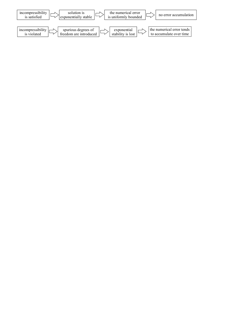
Figure 5: Summary of the main results.

The property of the exponential stability of the exact plastic flow was mathematically analyzed in this paper. Obviously, that property must be utilized during the development of new material models and corresponding algorithms in order to improve the accuracy and convergence of numerical computations.

Appendix A

Suppose $\Delta=\|\mathbf{\Delta}\|\rightarrow 0$. Let us show that

$$\rho_{\scriptscriptstyle\text{R}}\psi_{\text{el}}(\mathbf{1}+\mathbf{\Delta})=\frac{k}{8}(\text{tr}\mathbf{\Delta})^{2}+\frac{\mu}{4}\text{tr}\big{(}(\mathbf{\Delta}^{\text{D}})^{2}\big{)}+O(\Delta^{3}).$$ (93)

First, recall the Taylor expansion of $\det(\mathbf{1}+\mathbf{\Delta})$ up to second order

$$\det(\mathbf{1}+\mathbf{\Delta})=1+\text{tr}(\mathbf{\Delta})+1/2(\text{tr}(\mathbf{\Delta}))^{2}-1/2\text{tr}(\mathbf{\Delta}^{2})+O(\Delta^{3}).$$ (94)

Therefore,

$$\sqrt{\det(\mathbf{1}+\mathbf{\Delta})}=1+1/2\text{tr}(\mathbf{\Delta})+O(\Delta^{2}),$$ (95)

$$\frac{k}{2}\big{(}\text{ln}\sqrt{\det(\mathbf{1}+\mathbf{\Delta})}\big{)}^{2}=\frac{k}{8}(\text{tr}\mathbf{\Delta})^{2}+O(\Delta^{3}).$$ (96)

Next, note that for small $\varepsilon$ we have

$$(1+\varepsilon)^{-1/3}=1-1/3\varepsilon+2/9\varepsilon^{2}+O(\varepsilon^{3}).$$ (97)

Combining this with (94), we get

$$\frac{\mu}{2}\big{(}\text{tr}(\overline{\mathbf{1}+\mathbf{\Delta}})-3\big{)}=\frac{\mu}{2}\big{(}(\det(\mathbf{1}+\mathbf{\Delta}))^{-1/3}\text{tr}(\mathbf{1}+\mathbf{\Delta})-3\big{)}\\ =\frac{\mu}{2}\big{(}(1-1/3\text{tr}\mathbf{\Delta}+1/18(\text{tr}\mathbf{\Delta})^{2}+1/6\text{tr}(\mathbf{\Delta}^{2})+O({\Delta}^{3}))(3+\text{tr}\mathbf{\Delta})-3\big{)}\\ =\frac{\mu}{4}\big{(}\text{tr}(\mathbf{\Delta}^{2})-1/3(\text{tr}\mathbf{\Delta})^{2}\big{)}+O({\Delta}^{3})=\frac{\mu}{4}\text{tr}\big{(}(\mathbf{\Delta}^{\text{D}})^{2}\big{)}+O({\Delta}^{3}).$$ (98)

Finally, (93) follows from (33), using (96) and (98).

Appendix B

Let $\mathbf{A},\mathbf{B}\in M$ and $\|\mathbf{A}-\mathbf{B}\|\rightarrow 0$. Let us prove, for instance, that

$$\mathbf{B}^{-1}:(\mathbf{A}-\mathbf{B})=O(\|\mathbf{A}-\mathbf{B}\|^{2}).$$ (99)

Indeed, since $\det(\cdot)$ is a smooth function, we have

$$\det(\mathbf{A})=\det(\mathbf{B})+\frac{\displaystyle\partial\det(\mathbf{B})}{\displaystyle\partial\mathbf{B}}:(\mathbf{A}-\mathbf{B})+O(\|\mathbf{A}-\mathbf{B}\|^{2}).$$ (100)

Next, using the Jacobi formula, we get

$$\det(\mathbf{A})=\det(\mathbf{B})+\det(\mathbf{B})\mathbf{B}^{-\text{T}}:(\mathbf{A}-\mathbf{B})+O(\|\mathbf{A}-\mathbf{B}\|^{2}).$$ (101)

Finally, taking into account that $\det(\mathbf{A})=\det(\mathbf{B})=1$ and $\mathbf{B}^{-\text{T}}=\mathbf{B}^{-1}$, we obtain (99).

Remark. Note that for the tangential space $T_{\mathbf{B}}M$ to the manifold $M$ in $Sym$ we have

$$T_{\mathbf{B}}M=\{\mathbf{X}\in Sym\ |\ \mathbf{B}^{-1}:\mathbf{X}=0\}.$$ (102)

Thus, relation (99) implies that $\lim\limits_{\mathbf{A}\rightarrow\mathbf{B}}\big{(}(\mathbf{A}-\mathbf{B})/\|\mathbf{A}-\mathbf{B}\|\big{)}\in T_{\mathbf{B}}M$ (if the limit exists).

Appendix C

We need to construct a function $q(\theta)$ such that for small $\Delta$

$$q(\theta)\geq\Phi(\mathbf{C}^{(1)}_{\text{i}},\mathbf{C}^{(2)}_{\text{i}})+O(\Delta)\quad\text{for all}\ (\mathbf{C}^{(1)}_{\text{i}},\mathbf{C}^{(2)}_{\text{i}})\in S(\theta,\Delta).$$ (103)

Let $(\mathbf{C}^{(1)}_{\text{i}},\mathbf{C}^{(2)}_{\text{i}})\in S(\theta,\Delta)$. It follows from Appendix B, that

$$\big{(}\mathbf{C}^{(1)-1}_{\text{i}}-\mathbf{C}^{(2)-1}_{\text{i}}\big{)}:\mathbf{C}^{(1)}_{\text{i}}=O(\Delta^{2}).$$ (104)

By $\mathbf{X}$ denote the orthogonal projection of $\mathbf{C}^{(1)-1}_{\text{i}}-\mathbf{C}^{(2)-1}_{\text{i}}$ on the tangential space $T_{\mathbf{C}^{(1)-1}_{\text{i}}}M$. Using $\eqref{AppC2}$, we get for $\mathbf{X}$

$$\mathbf{X}=\mathbf{C}^{(1)-1}_{\text{i}}-\mathbf{C}^{(2)-1}_{\text{i}}-\Big{[}\big{(}\mathbf{C}^{(1)-1}_{\text{i}}-\mathbf{C}^{(2)-1}_{\text{i}}\big{)}:\mathbf{C}^{(1)}_{\text{i}}\frac{1}{\|\mathbf{C}^{(1)}_{\text{i}}\|^{2}}\Big{]}\mathbf{C}^{(1)}_{\text{i}}=\mathbf{C}^{(1)-1}_{\text{i}}-\mathbf{C}^{(2)-1}_{\text{i}}+O(\Delta^{2}).$$ (105)

Moreover, since $\text{tr}\big{(}\mathbf{X}\mathbf{C}^{(1)}_{\text{i}}\mathbf{X}\big{)}=\|\mathbf{X}(\mathbf{C}^{(1)}_{\text{i}})^{1/2}\|^{2}$, we have

$$\frac{O(\Delta^{3})}{\text{tr}\big{(}\mathbf{X}\mathbf{C}^{(1)}_{\text{i}}\mathbf{X}\big{)}}=O(\Delta).$$ (106)

Substituting (105) in (68) and taking (106) into account, we obtain

$$\Phi(\mathbf{C}^{(1)}_{\text{i}},\mathbf{C}^{(2)}_{\text{i}})=\frac{-2\big{(}\frac{(\mathbf{C}^{(1)-1}_{\text{i}})^{\text{D}}}{\|(\mathbf{C}^{(1)-1}_{\text{i}})^{\text{D}}\|}:\mathbf{X}\big{)}\big{(}\mathbf{1}:\mathbf{X}\big{)}}{\text{tr}\big{(}\mathbf{X}\mathbf{C}^{(1)}_{\text{i}}\mathbf{X}\big{)}}+O(\Delta).$$ (107)

Thus, we define $q(\theta)$ as

$$q(\theta):=\max_{\|(\mathbf{C}^{(1)-1}_{\text{i}})^{\text{D}}\|\leq\theta}\hat{q}(\mathbf{C}^{(1)}),\quad\hat{q}(\mathbf{C}^{(1)}):=\max_{\mathbf{X}\in T_{\mathbf{C}^{(1)-1}_{\text{i}}}M}\frac{-2\big{(}\frac{(\mathbf{C}^{(1)-1}_{\text{i}})^{\text{D}}}{\|(\mathbf{C}^{(1)-1}_{\text{i}})^{\text{D}}\|}:\mathbf{X}\big{)}\big{(}\mathbf{1}:\mathbf{X}\big{)}}{\text{tr}\big{(}\mathbf{X}\mathbf{C}^{(1)}_{\text{i}}\mathbf{X}\big{)}}.$$ (108)

The function $\hat{q}(\mathbf{C}^{(1)}_{\text{i}})$ can be evaluated as follows. First, for each $\mathbf{X}$ introduce $\mathbf{Y}=\mathbf{X}(\mathbf{C}^{(1)}_{\text{i}})^{1/2}$. Next, define a vector space $T:=\{\mathbf{Y}\in Sym\ |\ (\mathbf{C}^{(1)}_{\text{i}})^{1/2}:\mathbf{Y}=0\}$. Thus,

$$\mathbf{X}\in T_{\mathbf{C}^{(1)-1}_{\text{i}}}M\quad\iff\mathbf{Y}\in T,$$ (109)

$$\text{tr}\big{(}\mathbf{X}\mathbf{C}^{(1)}_{\text{i}}\mathbf{X}\big{)}=\|\mathbf{Y}\|,\quad-2\frac{(\mathbf{C}^{(1)-1}_{\text{i}})^{\text{D}}}{\|(\mathbf{C}^{(1)-1}_{\text{i}})^{\text{D}}\|}:\mathbf{X}=\mathbf{B}_{1}:\mathbf{Y},\quad\mathbf{1}:\mathbf{X}=\mathbf{B}_{2}:\mathbf{Y},$$ (110)

where

$$\mathbf{B}_{1}:=-2(\mathbf{C}^{(1)}_{\text{i}})^{-1/2}\frac{(\mathbf{C}^{(1)-1}_{\text{i}})^{\text{D}}}{\|(\mathbf{C}^{(1)-1}_{\text{i}})^{\text{D}}\|},\quad\mathbf{B}_{2}:=(\mathbf{C}^{(1)}_{\text{i}})^{-1/2}.$$ (111)

Therefore,

$$\hat{q}(\mathbf{C}^{(1)}_{\text{i}})=\max_{\mathbf{Y}\in T,\|\mathbf{Y}\|=1}\Big{[}\big{(}\mathbf{B}_{1}:\mathbf{Y}\big{)}\big{(}\mathbf{B}_{2}:\mathbf{Y}\big{)}\Big{]}.$$ (112)

Next, we compute the orthogonal projections of $\mathbf{B}_{1}$ and $\mathbf{B}_{2}$ on $T$:

$$\mathbf{B}^{0}_{\text{k}}:=\mathbf{B}_{\text{k}}-\big{(}\mathbf{B}_{\text{k}}:(\mathbf{C}^{(1)}_{\text{i}})^{1/2}\big{)}(\mathbf{C}^{(1)}_{\text{i}})^{1/2}\frac{1}{\|(\mathbf{C}^{(1)}_{\text{i}})^{1/2}\|^{2}},\quad\text{k}\in\{1,2\}.$$ (113)

Thus,

$$\hat{q}(\mathbf{C}^{(1)}_{\text{i}})=\max_{\mathbf{Y}\in T,\|\mathbf{Y}\|=1}\Big{[}\mathbf{Y}:\text{sym}\big{(}\mathbf{B}^{0}_{1}\otimes\mathbf{B}^{0}_{2}\big{)}:\mathbf{Y}\Big{]}=\lambda_{\max}\big{(}\text{sym}\big{(}\mathbf{B}^{0}_{1}\otimes\mathbf{B}^{0}_{2}\big{)}\big{)},$$ (114)

where $\lambda_{\max}\big{(}\text{sym}\big{(}\mathbf{B}^{0}_{1}\otimes\mathbf{B}^{0}_{2}\big{)}\big{)}$ is the maximal eigenvalue of the symmetric operator
$\text{sym}\big{(}\mathbf{B}^{0}_{1}\otimes\mathbf{B}^{0}_{2}\big{)}:Sym\rightarrow Sym$. Obviously, the same maximal eigenvalue has its restriction on $T^{0}=\text{Span}\{\mathbf{B}^{0}_{1},\mathbf{B}^{0}_{2}\}$. It can be easily seen that

$$\text{sym}\big{(}\mathbf{B}^{0}_{1}\otimes\mathbf{B}^{0}_{2}\big{)}(\mathbf{B}^{0}_{1})=1/2(\mathbf{B}^{0}_{1}:\mathbf{B}^{0}_{2})\mathbf{B}^{0}_{1}+1/2(\mathbf{B}^{0}_{1}:\mathbf{B}^{0}_{1})\mathbf{B}^{0}_{2},$$ (115)

$$\text{sym}\big{(}\mathbf{B}^{0}_{1}\otimes\mathbf{B}^{0}_{2}\big{)}(\mathbf{B}^{0}_{2})=1/2(\mathbf{B}^{0}_{2}:\mathbf{B}^{0}_{2})\mathbf{B}^{0}_{1}+1/2(\mathbf{B}^{0}_{1}:\mathbf{B}^{0}_{2})\mathbf{B}^{0}_{2}.$$ (116)

Therefore, the matrix of the restricted operator with respect to the basis $\{\mathbf{B}^{0}_{1},\mathbf{B}^{0}_{2}\}$ has the following form

$$A:=\frac{1}{2}\left(\begin{array}[]{cc}\mathbf{B}^{0}_{1}:\mathbf{B}^{0}_{2}&\ \mathbf{B}^{0}_{2}:\mathbf{B}^{0}_{2}\\ \mathbf{B}^{0}_{1}:\mathbf{B}^{0}_{1}&\ \mathbf{B}^{0}_{1}:\mathbf{B}^{0}_{2}\end{array}\right).$$ (117)

Both eigenvalues of $A$ are real, since $A$ represents a symmetric tensor. Finally,

$$\hat{q}(\mathbf{C}^{(1)}_{\text{i}})=\lambda_{\max}\big{(}\text{sym}\big{(}\mathbf{B}^{0}_{1}\otimes\mathbf{B}^{0}_{2}\big{)}\big{)}=\lambda_{\max}(A).$$ (118)

Note that $\hat{q}(\mathbf{C}^{(1)}_{\text{i}})$ is a continuous function of $\mathbf{C}^{(1)}_{\text{i}}$. Therefore, the maximum $q(\theta)=\max\limits_{\|(\mathbf{C}^{(1)-1}_{\text{i}})^{\text{D}}\|\leq\theta}\hat{q}(\mathbf{C}^{(1)})$ is well defined. We compute it by the brutal force method. Moreover, the following parametrization can be used to simplify the computations. For any tensor $\mathbf{C}^{(1)}_{\text{i}}$ there exists a cartesian coordinate system and real numbers $\lambda^{1},\lambda^{2}>0$ such that the matrix of $\mathbf{C}^{(1)}_{\text{i}}$ takes the diagonal form $\text{diag}(\lambda^{1},\lambda^{2},1/(\lambda^{1}\lambda^{1}))$. The function $q(\theta)$ is plotted on the figure 6 for $0\leq\theta\leq 0.03$.

\psfrag{A}[m][1][0]{$\theta$}\psfrag{B}[m][1][0]{$q$}\includegraphics{fig5.eps}

Figure 6: Function $q(\theta)$.

References

• [1] H. D. Alber, Materials With Memory. Initial-Boundary Value Problems for Constitutive Equations with Internal Variables (Springer, 1997).
• [2] N. S. Bahvalov, N. P. Jidkov, G. M. Kobelkov. Numerical methods. [in Russian] (Lab of base knowledge, 2001).
• [3] A. Bertram, Elasticity and Plasticity of Large Deformations (Springer, 2005).
• [4] W. Dettmer, S. Reese, On the theoretical and numerical modelling of Armstrong -Frederick kinematic hardening in the finite strain regime, Computer Methods in Applied Mechanics and Engineering, 193 (2004) 87 -116.
• [5] U. J. Görke, A. Bucher, R. Kreißig, A study on kinematic hardening models for the simulation of cyclic loading in finite elasto-plasticity based on a substructure approach, In: Owen, D.R.J., Onate, E. and Suarez, B. (Eds.): Computational Plasticity: Fundamentals and Applications. Proceedings of COMPLAS VIII, CIMNE Barcelona, (2005) 723–726.
• [6] E. Hairer, Geometric Integration of Ordinary Differential Equations on Manifolds, BIT Numerical Mathematics, 41, 5 (2001) 996–1007.
• [7] E. Hairer, C. Lubich, G. Wanner, Geometric Numerical Integration. Structure Preserving Algorithms for Ordinatry Differential Equations (Springer, 2006).
• [8] W. Han, B. D. Reddy, Plasticity. Mathematical Theory and Numerical Analysis. (Springer, 1999).
• [9] S. Hartmann, G. Lührs, P. Haupt, An efficient stress algorithm with applications in viscoplasticity and plasticity, International Journal for Numerical Methods in Engineering, 40 (1997) 991–1013.
• [10] S. Hartmann, K. J. Quint, M. Arnold, On plastic incompressibility within time-adaptive finite elements combined with projection techniques, Computer Methods in Applied Mechanics and Engineering, 198 (2008) 178–173.
• [11] P. Haupt, Continuum Mechanics and Theory of Materials, 2nd edition, Springer, 2002.
• [12] D. Helm, Formgedächtnislegierungen, experimentelle Untersuchung, phänomenologische Modellierung und numerische Simulation der thermomechanischen Materialeigenschaften, Universitätsbibliothek Kassel, 2001.
• [13] D. Helm, Stress computation in finite thermoviscoplasticity. International Journal of Plasticity, 22 (2006) 1699–1721.
• [14] I. R. Ionescu, M. Sofonea, Functional and Numerical Methods in Viscoplasticity, 1. ed. Oxford Mathematical Monographs (Oxford University Press, 1993.)
• [15] M. Itskov, Tensor Algebra and Tensor Analysis for Engineers: With Applications to Continuum Mechanics (Springer, 2007).
• [16] J. Kato, A. A. Martynyuk, A. A. Shestakov, Stability of Motion of Nonautonomous Systems (Method of Limiting Equations), Stability and Control: Theory Methods and Applications, Volume 3, (Gordon and Breach Publishers, 1996).
• [17] E. Kröner, Allgemeine Kontinuumstheorie der Versetzungen und Eigenspannungen, Arch. Rational Mech. Anal., 4 (1959) 273-334.
• [18] E. H. Lee, Elastic -plastic deformation at finite strains, J. Appl. Mech., 36 (1969) 1-6.
• [19] A. Lion, Constitutive modelling in finite thermoviscoplasticity: a physical approach based on nonlinear rheological elements, International Journal of Plasticity, 16 (2000) 469–494.
• [20] G. Lührs, S. Hartmann, P. Haupt, On the numerical treatment of finite deformations in elastoviscoplasticity, Computer Methods in Applied Mechanics and Engineering, 144 (1997) 1- 21.
• [21] R. Michel, R. Kreißig, H. Ansorge, Thermomechanical finite element analysis (FEA) of spin extrusion, Forschung im Ingenieurwesen, 68 (2003) 19–24
• [22] C. Miehe, E. Stein, A canonical model of multiplicative elasto-plasticity: formulation and aspects of the numerical implementation, European Journal of Mechanics A/Solids, 11 (1992) 25–43
• [23] C. Miehe, Exponential map algorithm for stress updates in anisotropic multiplicative elastoplasticity for single crystals, International Journal for Numerical Methods in Engineering, 39 (1996) 3367–3390.
• [24] P. Neff, Mathematische Analyse multiplikativer Viskoplastizität. Ph.D. Thesis TU Darmstadt. (Shaker Verlag, 2000).
• [25] P. Perzyna. The constitutive equations for rate sensitive plastic materials, Quarterly of Applied Mathematics, 20 (1963) 321–331.
• [26] P. Perzyna, Fundamental problems in visco-plasticity, G. Kuerti (Ed.), Advances in Applied Mechanics, vol. 9, Academic Press, New York, (1966) 243–377.
• [27] A.  V. Shutov, R. Kreißig, Finite strain viscoplasticity with nonlinear kinematic hardening: Phenomenological modeling and time integration, Computer Methods in Applied Mechanics and Engineering, 197, 2015–2029 (2008).
• [28] A.  V. Shutov, R. Kreißig, Application of a coordinate-free tensor formalism to the numerical implementation of a material model, ZAMM, 88, 11, 888-909 (2008).
• [29] J. Simo, T. Hughes, Computational inelasticity, Springer, 1998.
• [30] J. C. Simo, C. Miehe, Associative coupled thermoplasticity at finite strains: formulation, numerical analysis and implementation, Computer Methods in Applied Mechanics and Engineering, 98 (1992) 41 -104.
• [31] B. Svendsen, A logarithmic- exponential backward-Euler-based split of the flow rule for anisotropic inelastic behaviour at small elastic strain, International Journal for Numerical Methods in Engineering, 70, 496-504 (2007).
• [32] C. Truesdell, W. Noll, The Non-Linear Field Theories of Mechanics, 2nd ed. (Springer, 1992).
• [33] G. Vadillo, R. Zaera, J. Fernandez-Saez, Consistent integration of the constitutive equations of Gurson materials under adiabatic conditions, Computer Methods in Applied Mechanics and Engineering, 197, 1280-1295 (2008).
• [34] R. Z. Valiev, R. K. Islamgaliev, I. V. Alexandrov, Bulk nanostructured materials from severe plastic deformation, Progress in Materials Science, 45, 103-189 (2000).
• [35] G. Weber, L. Annand, Finite deformation constitutive equations and a time integration procedure for isotropic, hyperelastic-viscoelastic solids, Computer Methods in Applied Mechanics and Engineering, 79 (1990) 173-202.