Correlated electron physics in multilevel quantum dots:
phase transitions, transport, and experiment.

Abstract

We study correlated two-level quantum dots, coupled in effective 1-channel fashion to metallic leads; with electron interactions including on-level and inter-level Coulomb repulsions, as well as the inter-orbital Hund’s rule exchange favoring the spin-1 state in the relevant sector of the free dot. For arbitrary dot occupancy, the underlying phases, quantum phase transitions (QPTs), thermodynamics, single-particle dynamics and electronic transport properties are considered; and direct comparison is made to conductance experiments on lateral quantum dots. Two distinct phases arise generically, one characterised by a normal Fermi liquid fixed point (FP), the other by an underscreened (USC) spin-1 FP. Associated QPTs, which occur in general in a mixed valent regime of non-integral dot charge, are found to consist of continuous lines of Kosterlitz-Thouless transitions, separated by first order level-crossing transitions at high symmetry points. A ‘Friedel-Luttinger sum rule’ is derived and, together with a deduced generalization of Luttinger’s theorem to the USC phase (a singular Fermi liquid), is used to obtain a general result for the $T=0$ zero-bias conductance, expressed solely in terms of the dot occupancy and applicable to both phases. Relatedly, dynamical signatures of the QPT show two broad classes of behavior, corresponding to the collapse of either a Kondo resonance, or antiresonance, as the transition is approached from the Fermi liquid phase; the latter behavior being apparent in experimental differential conductance maps. The problem is studied using the numerical renormalization group method, combined with analytical arguments.

I Introduction

The Kondo effect is one of the enduring paradigms of quantum many-body theory Hewson (1993). For most of its history it has been associated with bulk condensed matter, notably transition metal impurites dissolved in clean metals, and certain heavy fermion rare earth compounds Hewson (1993). In recent years, however, the advent of quantum dot systems – with the impressive control and tunability possible for ‘artificial atoms’ – has generated a strong resurgence of interest in Kondo and related physics in nanoscale devices (for reviews see e.g. [Kouwenhoven et al., 1997; Pustilnik and Glazman, 2004]).

In odd-electron quantum dots the spin-$1/2$ Kondo effect arises. Manifest experimentally Goldhaber-Gordon et al. (1998); Cronenwett et al. (1998) as a strong low-temperature enhancement of the zero bias conductance, indicating the formation of the local Kondo singlet below a characteristic Kondo temperature, the basic theoretical model here is of course the Anderson impurity model Anderson (1961): a single dot level, with a single on-level Coulomb interaction, tunnel coupled to non-interacting metallic leads. Moreover the Anderson model captures not only the Kondo regime – arising towards the center of the associated Coulomb blockade valley where the dot level is singly occupied – but also the mixed valent regimes of non-integral occupancy occurring towards the edges of the valley. As such, it encompasses essentially all the physics associated with a single ‘active’ dot level.

The situation is naturally more complex, and richer, if two active dot levels are integral to electronic transport. For example, higher dot spin states now become possible, in this case a 2-electron triplet stabilised by the inter-orbital Hund’s rule exchange Brouwer et al. (1999); Baranger et al. (2000). This state has been observed experimentally in even-electron dots, for both lateral Schmid et al. (2000); van der Wiel et al. (2002); Kogan et al. (2003); Quay et al. (2007) and vertical Sasaki et al. (2000) devices (as well as in a single-molecule dot Roch et al. (2008)). It too is manifest in a strong enhancement of the zero-bias conductance, indicative Pustilnik and Glazman (2001); Posazhennikova et al. (2007) of proximity to an underscreened spin-1 fixed point Nozières and Blandin (1980) in which the spin-$1$ is quenched to an effective spin-$\tfrac{1}{2}$ on coupling to the leads.

Much important theoretical work on the problem has ensued; including both the 1-channel case (see e.g. [Kikoin and Avishai, 2001; Hofstetter and Schoeller, 2001; Vojta et al., 2002; Koller et al., 2005; Pustilnik and Borda, 2006; Posazhennikova and Coleman, 2005; Posazhennikova et al., 2007; Bas and Aligia, 2009]) where the single screening channel yields underscreened (USC) spin-$1$ as the stable low-temperature fixed point, and the 2-channel case Pustilnik and Glazman (2000, 2001); Pustilnik et al. (2003); Hofstetter and Zarand (2004); Posazhennikova and Coleman (2005); Posazhennikova et al. (2007) where the spin-$1$ local moment is fully screened at the lowest temperatures. Further, since the USC spin-1 fixed point is clearly distinct from that characteristic of a normal Fermi liquid – the USC phase being a ‘singular Fermi liquid’ Mehta et al. (2005) – quantum phase transitions from a normal Fermi liquid to the USC phase are expected, and found, to arise in the 1-channel case (with pristine transitions broadened into crossovers for 2-channel screening). This too has been studied quite extensively Kikoin and Avishai (2001); Hofstetter and Schoeller (2001); Vojta et al. (2002); Pustilnik and Borda (2006); Bas and Aligia (2009); Pustilnik and Glazman (2000); Pustilnik et al. (2003); Hofstetter and Zarand (2004). However the large majority of previous work on these ‘singlet-triplet’ transitions has focussed on a somewhat particular case – the middle of the 2-electron Coulomb blockade valley where, throughout both phases, the dot occupancy/charge remains close to 2; a situation we regard as unlikely to be applicable to a transition driven by tuning a gate voltage in the absence of a magnetic field (as in the experiments e.g. of [Kogan et al., 2003]), where one instead expects the dot charge to vary continuously with gate voltage. A notable exception is the work of [Pustilnik and Borda, 2006], in which low-temperature transport is considered in a region separating two adjacent Coulomb blockade valleys with spins $S=\tfrac{1}{2}$ and $S=1$ on the dot, and where the resultant quantum phase transition, driven by gate voltage and arising in the limit $B\rightarrow 0+$ of vanishing magnetic field, occurs in a mixed valent regime of non-integral dot charge.

In view of the above our aim here is to consider a rather general model of a two-level quantum dot, coupled in a 1-channel fashion to metallic leads; to consider its underlying phases, thermodynamics, single-particle dynamics and associated low-temperature ($T$) electronic transport, for arbitrary dot charge – spanning as such the full range of possible behavior; and ultimately to make tangible comparison to experiment Kogan et al. (2003). The model itself is specified in sec. II and reflects the natural complexity of a two-level dot, where in addition to the one-electron dot levels electron interactions include both on-level and inter-level Coulomb repulsions, together with inter-orbital spin-exchange. We study it using Wilson’s numerical renormalization group (NRG) technique Wilson (1975); Krishnamurthy et al. (1980a, b) as the method of choice, employing the full density matrix formulation of the method Peters et al. (2006); Weichselbaum and von Delft (2007) (for a recent review see [Bulla et al., 2008]); together where possible with analytical arguments.

The intrinsic phases and associated thermodynamics are considered in sec. III. With $\epsilon_{1}$, $\epsilon_{2}$ denoting the one-electron level energies, the general structure of the phase diagrams in the ($\epsilon_{1},\epsilon_{2}$)-plane is found to consist of a closed, continuous line of quantum phase transitions (QPTs) separating an USC spin-1 phase from a continuously connected normal Fermi liquid phase; although more complex topologies arise as the exchange coupling is driven weakly antiferromagnetic (sec. III.2), leading ultimately to destruction of the USC phase. The transitions are found in general to be of Kosterlitz-Thouless type, except for particular lines of symmetry where first order, level-crossing transitions arise (sec. III.1).

Sec. IV focusses on the $T=0$ zero-bias conductance $G_{c}$, and associated static phase shift $\delta$. A ‘Friedel-Luttinger sum rule’ for $\delta$ is derived, applicable to both the normal Fermi liquid and the USC spin-1 phases, and reducing to the usual Friedel sum rule Langreth (1966); Hewson (1993) in the Fermi liquid phase. Since the USC phase is a singular Fermi liquid Mehta et al. (2005), and as such not perturbatively connected to the non-interacting limit of the model, one does not expect Luttinger’s (integral) theorem Luttinger (1960) to apply. A generalization of it for the USC phase is however deduced, and its important consequences for the zero-bias conductance considered; leading to a simple result which, for both the normal Fermi liquid and USC phases, gives $G_{c}$ in terms of the dot occupancy/charge (or, strictly, the ‘excess impurity charge’ Hewson (1993)).

Single-particle dynamics for both phases are detailed in sec. V. In particular, dynamical signatures of the QPT on approaching it from the normal Fermi liquid are found to fall into two broad classes, corresponding respectively to an ‘on the spot’ vanishing of either a Kondo resonance, or a Kondo antiresonance, in the single-particle spectrum; the spectral collapse in either case being associated with a vanishing Kondo scale $T_{K}$ as the transition is approached, and in terms of which universal scaling of dynamics is found to occur.

Finally, in sec. VI we make explicit comparison to the experiments of [Kogan et al., 2003] on a lateral dot; in which, on continuous tuning of a gate voltage at zero magnetic field, both the normal spin-$1/2$ Fermi liquid and the USC spin-1 phase are observed in adjacent Coulomb blockade valleys. Both the zero-bias conductance as a function of gate voltage, and (in this case inevitably approximate) differential conductance maps as a function of both gate and bias voltages, are compared to experiment; and the features observed related to the dynamics considered in secs. (IV,V). We believe it fair to say that the underlying theory accounts rather well for experiment.

II Model

Interacting quantum dots and other nanodevices are described generally by the dot $\hat{H}_{\mathrm{D}}$, a pair of non-interacting leads $\hat{H}_{\mathrm{L}}$, and a tunnel coupling between the subsystems: $\hat{H}=\hat{H}_{\mathrm{D}}+\hat{H}_{\mathrm{L}}+\hat{H}_{\mathrm{T}}$. We consider in this work a two-level interacting quantum dot of form:

$$\hat{H}_{\mathrm{D}}~{}=~{}\sum_{i,\sigma}\left(\epsilon_{i}+\tfrac{1}{2}U\hat{n}_{i-\sigma}^{\phantom{\dagger}}\right)\hat{n}_{i\sigma}^{\phantom{\dagger}}+U^{\prime}\hat{n}_{1}^{\phantom{\dagger}}\hat{n}_{2}^{\phantom{\dagger}}-J_{\mathrm{H}}~{}\hat{\mathbf{s}}_{1}\cdot\hat{\mathbf{s}}_{2}$$ (1)

Here $\hat{n}_{i\sigma}^{\phantom{\dagger}}=d^{\dagger}_{i\sigma}d^{\phantom{\dagger}}_{i\sigma}$ where $d^{\dagger}_{i\sigma}$ creates a $\sigma$ ($=\uparrow,\downarrow$) spin electron in level $i$ ($=1,2$), $\hat{n}_{i}^{\phantom{\dagger}}=\sum_{\sigma}\hat{n}_{i\sigma}^{\phantom{\dagger}}$ is the total number operator for level $i$, and $\hat{\mathbf{s}}_{i}$ is the local spin-operator with components $\hat{\mathbf{s}}_{i}^{\alpha}=\sum_{\sigma,\sigma^{\prime}}d^{\dagger}_{i\sigma}\sigma^{(\alpha)}_{\sigma\sigma^{\prime}}d_{i\sigma^{\prime}}^{\phantom{\dagger}}$ and $\bm{\sigma}^{(\alpha)}$ the Pauli matrices. The single-particle levels have energies $\epsilon_{i}$, the on-level Coulomb interaction (taken to be the same for both levels) is denoted by $U$, and the inter-level interaction by $U^{\prime}$. Finally $J_{\mathrm{H}}$ is the exchange coupling, taken in accordance with Hund’s rule to be ferromagnetic ($J_{\mathrm{H}}>0$, although we also comment in sec. III.2 on the weakly antiferromagnetic case). The states arising from $\hat{H}_{\mathrm{D}}$ itself will be discussed in sec. II.2 below.

The Hamiltonian for the two equivalent non-interacting leads ($\nu=L,R$) is given by $\hat{H}_{\mathrm{L}}=\sum_{\nu}\sum_{\mathbf{k},\sigma}\epsilon_{\mathbf{k}}^{\phantom{\dagger}}a^{\dagger}_{\mathbf{k}\nu\sigma}a^{\phantom{\dagger}}_{\mathbf{k}\nu\sigma}$. Tunnel coupling to the leads is described generally by $\hat{H}_{\mathrm{T}}=\sum_{\nu}\sum_{i,\mathbf{k},\sigma}\mathrm{V}_{i\nu}^{\phantom{\dagger}}(d^{\dagger}_{i\sigma}a^{\phantom{\dagger}}_{\mathbf{k}\nu\sigma}+\mathrm{h.c.})$ where $\mathrm{V}_{i\nu}^{\phantom{\dagger}}$ is the tunnel coupling matrix element between dot level $i$ and lead $\nu$. We consider explicitly in this paper the case of an effective 1-channel setup, in which the ratio $V_{2\nu}^{\phantom{\dagger}}/V_{1\nu}^{\phantom{\dagger}}\equiv\mathrm{V}_{2}^{\phantom{\dagger}}/\mathrm{V}_{1}^{\phantom{\dagger}}$ is independent of the lead index $\nu$; i.e. the tunnel couplings are of form $\mathrm{V}_{iL}^{\phantom{\dagger}}=\alpha\mathrm{V}_{i}^{\phantom{\dagger}}$, $\mathrm{V}_{iR}^{\phantom{\dagger}}=\beta\mathrm{V}_{i}^{\phantom{\dagger}}$ (with $\alpha^{2}+\beta^{2}=1$), as illustrated schematically in fig. 1. A simple canonical transformation to new lead orbitals may then be performed, $c^{\phantom{\dagger}}_{\mathbf{k}\sigma}=\alpha a^{\phantom{\dagger}}_{\mathbf{k}L\sigma}+\beta a^{\phantom{\dagger}}_{\mathbf{k}R\sigma}$ and $\tilde{c}_{\mathbf{k}\sigma}^{\phantom{\dagger}}=-\beta a^{\phantom{\dagger}}_{\mathbf{k}L\sigma}+\alpha a^{\phantom{\dagger}}_{\mathbf{k}R\sigma}$, such that solely the bonding combination of lead states ($c^{\phantom{\dagger}}_{\mathbf{k}\sigma}$) couples to the dot:

$$\hat{H}_{\mathrm{T}}~{}=~{}\sum_{i,\mathbf{k},\sigma}\mathrm{V}_{i}^{\phantom{\dagger}}(d^{\dagger}_{i\sigma}c^{\phantom{\dagger}}_{\mathbf{k}\sigma}+\mathrm{h.c.})$$ (2)

We can thus drop the lead index $\nu$ and consider one effective lead

$$\hat{H}_{\mathrm{L}}~{}=~{}\sum_{\mathbf{k},\sigma}\epsilon_{\mathbf{k}}^{\phantom{\dagger}}c^{\dagger}_{\mathbf{k}\sigma}c^{\phantom{\dagger}}_{\mathbf{k}\sigma}~{},$$ (3)

hence the effective 1-channel description illustrated in fig. 1. In practice we consider the standard case Hewson (1993) of a symmetric, flat-band conduction band with half bandwidth $D$, i.e. the lead density of states (per conduction orbital) is $1/(2D)$.

It need hardly be added that the tunnel coupling pattern considered (fig. 1) is not the most general case, which would by contrast involve an irreducibly 2-channel description Pustilnik and Glazman (2001), in general with strong channel anisotropy Pustilnik and Glazman (2001); Posazhennikova et al. (2007). The richness of the physics arising in the case considered, with its associated pristine QPTs, is nonetheless more than ample to justify its study (indeed for NRG calculations in practice, we focus largely on the case $\mathrm{V}_{2}^{\phantom{\dagger}}=\mathrm{V}_{1}^{\phantom{\dagger}}$). It has moreover been argued (see e.g. [Hofstetter and Schoeller, 2001; Vojta et al., 2002]) that the 1-channel case is generally appropriate to lateral quantum dots, while a 2-channel model is appropriate for vertical dots.

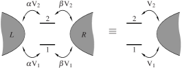
Figure 1: Schematic of the two-level dot (levels 1,2) coupled to the $\nu=L,R$ leads with the tunnel couplings $V_{2\nu}/V_{1\nu}\equiv V_{2}/V_{1}$ independent of $\nu$; leading to the equivalent one-lead description indicated.

In considering equilibrium electronic transport per se, the central quantity is of course the zero-bias conductance, $G_{c}(T)$, across the $L/R$ leads (fig. 1). An expression for it is readily obtained following Meir and Wingreen Meir and Wingreen (1992), and is:

$$G_{\mathrm{c}}(T)~{}=~{}\frac{2e^{2}}{h}G_{0}\int^{\infty}_{-\infty}d\omega~{}\frac{-\partial f(\omega)}{\partial\omega}~{}\pi(\Gamma_{11}+\Gamma_{22})~{}D_{ee}(\omega)$$ (4)

Here $f(\omega)=[e^{\omega/T}+1]^{-1}$ ($k_{B}\equiv 1$) is the Fermi function and

$$\Gamma_{ii}~{}=~{}\pi\rho\mathrm{V}_{i}^{\phantom{\dagger}2}$$ (5)

is the hybridization strength for level $i$ ($\rho$ is the lead density of states). The dimensionless conductance prefactor $G_{0}=(2\alpha\beta)^{2}$ – or equivalently $G_{0}=4\Gamma_{L}\Gamma_{R}/(\Gamma_{L}+\Gamma_{R})^{2}$ with $\Gamma_{\nu}=\pi\rho\sum_{i}\mathrm{V}_{i\nu}^{\phantom{\dagger}2}$ – reflects the relative asymmetry in tunnel coupling to the $L/R$ leads. It is naturally maximal, $G_{0}=1$, for symmetric coupling where (fig. 1) $\alpha=1/\sqrt{2}=\beta$ (i.e. $\Gamma_{R}=\Gamma_{L}$). The key quantity determining the conductance eqn. (4), which we analyse in detail in later sections, is the ‘even-even’ single-particle spectrum: $D_{ee}(\omega)=-\tfrac{1}{\pi}\mathrm{Im}G_{ee}(\omega)$ in terms of the (retarded) Green function $G_{ee}(\omega)$ ($\leftrightarrow G_{ee}(t)=-\mathrm{i}\theta(t)\langle\{d_{e\sigma}^{\phantom{\dagger}}(t),d_{e\sigma}^{\dagger}\}\rangle$). The $e$-orbital creation operator is given generally by

$$d_{e\sigma}^{\dagger}~{}=~{}\frac{1}{\sqrt{\Gamma_{11}+\Gamma_{22}}}\left(\sqrt{\Gamma_{11}}~{}d_{1\sigma}^{\dagger}~{}+~{}\sqrt{\Gamma_{22}}~{}d_{2\sigma}^{\dagger}\right)$$ (6)

in terms of the level creation operators, such that

$$G_{ee}(\omega)~{}=~{}\frac{1}{\Gamma_{11}+\Gamma_{22}}~{}\sum_{i,j}~{}\Gamma_{ij}~{}G_{ij}(\omega)$$ (7)

in terms of the corresponding propagators for the dot levels, $G_{ij}(\omega)$ ($i,j\in{\{1,2\}}$); and where

$$\Gamma_{12}~{}=~{}\pi\rho\mathrm{V}_{1}^{\phantom{\dagger}}\mathrm{V}_{2}^{\phantom{\dagger}}~{}~{}~{}\equiv\sqrt{\Gamma_{11}\Gamma_{22}}$$ (8)

is the inter-level hybridization strength.

For the case $\mathrm{V}_{2}^{\phantom{\dagger}}=\mathrm{V}_{1}^{\phantom{\dagger}}$ all hybridization strengths coincide,

$$\Gamma_{ij}~{}\equiv~{}\Gamma~{}~{}~{}~{}~{}~{}~{}~{}:\mathrm{V}_{2}^{\phantom{\dagger}}=\mathrm{V}_{1}^{\phantom{\dagger}}$$ (9)

(and the $e$-$e$ propagator then reduces simply to $G_{ee}(\omega)=\tfrac{1}{2}[G_{11}(\omega)+G_{22}(\omega)+2G_{12}(\omega)]$). It is convenient in this case to specify the ‘bare’ parameters of $\hat{H}_{\mathrm{D}}$ in terms of $\Gamma$, defining

$$\tilde{\epsilon_{i}}=\frac{\epsilon_{i}}{\Gamma},~{}~{}~{}~{}~{}\tilde{U}=\frac{U}{\Gamma},~{}~{}~{}~{}~{}\tilde{U^{\prime}}=\frac{U^{\prime}}{\Gamma},~{}~{}~{}~{}~{}\tilde{J}_{\mathrm{H}}=\frac{J_{\mathrm{H}}}{\Gamma}~{}.$$ (10)

II.1 Symmetries

We will subsequently consider different phases of the dot-lead coupled system in the ($\epsilon_{1},\epsilon_{2}$)-plane, for given values of the interaction parameters $U,U^{\prime}$ and $J_{\mathrm{H}}$ entering $\hat{H}_{\mathrm{D}}$ (eqn. (1)). To this end it is economical to exploit symmetry. Rather than the bare levels $\epsilon_{1},\epsilon_{2}$ it is often helpful to employ

$$x~{}=~{}\epsilon_{1}~{}+~{}\tfrac{1}{2}U~{}+~{}U^{\prime}$$ (11a)

$$y~{}=~{}\epsilon_{2}~{}+~{}\tfrac{1}{2}U~{}+~{}U^{\prime}~{}.$$ (11b)

Their significance arises from a particle-hole transformation ($p$-$ht$) of $\hat{H}=\hat{H}_{\mathrm{D}}+\hat{H}_{\mathrm{L}}+\hat{H}_{\mathrm{T}}$ (eqns. (1 - 3)), namely Krishnamurthy et al. (1980a)

$$d^{\phantom{\dagger}}_{i\sigma}~{}\rightarrow~{}d^{\dagger}_{i\sigma}~{}~{}~{}~{}~{}~{}~{}c^{\phantom{\dagger}}_{\mathbf{k}\sigma}\rightarrow-c^{\dagger}_{-\mathbf{k}\sigma}~{}.$$ (12)

$\hat{H}\equiv\hat{H}(x,y)$ transforms under the $p$-$ht$ as $\hat{H}(x,y)\rightarrow 2(x+y)+\hat{H}(-x,-y)$, and is hence invariant at the $p$-$h$ symmetric point $x=0=y$. Use of $x,y$ thus specifies the level energies relative to this point. All physical properties, thermodynamic and dynamic, have characteristic symmetries under the $p$-$ht$, which we exploit many times in the paper. For example the free energy $F(x,y)=-T\ln\{\mathrm{Tr}~{}e^{-\beta\hat{H}(x,y)}\}$ is, modulo an irrelevant constant, equivalent to its $p$-$ht$ counterpart ($F(x,y)=2(x+y)+F(-x,-y)$), whence e.g. phase boundaries (secs. (II.2,III)) are invariant under inversion $(x,y)\rightarrow(-x,-y)$; and thus only $y\geq x$ need in practice be considered.

The second symmetry exploited is a ‘$1$-$2$’ transformation, viz. the trivial canonical transformation

$$(d_{1\sigma}^{\phantom{\dagger}},d_{2\sigma}^{\phantom{\dagger}})~{}\rightarrow~{}(d_{2\sigma}^{\phantom{\dagger}},d_{1\sigma}^{\phantom{\dagger}})~{}$$ (13)

under which the dot Hamiltonian $\hat{H}_{\mathrm{D}}(x,y)\rightarrow\hat{H}_{\mathrm{D}}(y,x)$. The same symmetry applies to the full $\hat{H}$ for $\mathrm{V}_{2}^{\phantom{\dagger}}=\mathrm{V}_{1}^{\phantom{\dagger}}$; whence e.g. $F(x,y)=F(y,x)$ is invariant to reflection about the line $y=x$, and in consequence phase boundaries need overall be considered only for $y\geq|x|$.

Figure 2: (a)-(c) show ground states of the isolated dot in the ($x,y$)-plane, for $U=20$ and $J_{\mathrm{H}}=5$ (in units of $\Gamma\equiv 1$); with (a) $U^{\prime}=7.5$, (b) $U^{\prime}=0$ and (c) $U^{\prime}=U$. States are labelled as $(n_{1},n_{2})$, with $n_{i}=\langle\hat{n}_{i}\rangle$ the charge on level $i$. Phase boundaries surrounding the 2-electron triplet state $(n_{1},n_{2})=(1,1)$) are indicated by solid lines, and all others by dotted lines. The dashed arrowed line in (a) shows the form of an experimental ‘trajectory’ on application of a gate voltage, see text. For the same bare parameters as (a), Fig. 2(d) shows the phase diagram obtained via NRG for the lead-coupled dot system (with $V_{2}=V_{1}$), as detailed in sec. III ff. It consists of a line of continuous quantum phase transitions (thick solid line) and two first order level-crossing transitions on the line $y=x$ (shown as dots), separating a singular Fermi liquid phase Mehta et al. (2005) characterised by an underscreened spin-1 fixed point Nozières and Blandin (1980) (interior, ‘USC’) from a normal Fermi liquid (‘FL’) characterised in general by a frozen impurity FP Krishnamurthy et al. (1980b). The hexagonal boundary of the $(1,1)$ triplet state for the isolated dot (fig. 2(a)) is also shown for comparison.

II.2 Ground state phases: overview

It is first instructive to consider briefly the states of the isolated dot in the ($x,y$)-plane, as determined by the ground states of $\hat{H}_{\mathrm{D}}$ (eqn. (1)). We label the dot states as ($n_{1},n_{2}$) (with $n_{i}=\langle\hat{n}_{i}^{\phantom{\dagger}}\rangle$ the ground state charge for level $i$), with energies $E_{D}(n_{1},n_{2})$. For all $J_{\mathrm{H}}>0$, the 2-electron dot ground state is the ($1,1$) spin triplet with energy $E_{T}$ ($\equiv E_{D}(1,1)=\epsilon_{1}+\epsilon_{2}+U^{\prime}-\tfrac{1}{4}J_{\mathrm{H}}$), centred on the $p$-$h$ symmetric point $(x,y)=(0,0)$; as illustrated in fig. 2(a) for the representative case $U=20$, $U^{\prime}=7.5$ and $J_{\mathrm{H}}=5$. All other ground states, indicated in the figure, are either spin singlets or doublets.

Considering in particular $y\geq|x|$ – phase boundaries being invariant to inversion and reflection as above – the ($1,1$) triplet is bordered both by another 2-electron state, viz. the spin singlet ($2,0$), and by a 1-electron spin doublet ($1,0$) (the bounding lines for which are given by $y=x+U-U^{\prime}+\tfrac{1}{4}J_{\mathrm{H}}$ and $y=\tfrac{1}{2}U+\tfrac{1}{4}J_{\mathrm{H}}$ respectively). The dashed line in fig. 2(a) shows a typical ‘trajectory’, $y=x+\Delta\epsilon$ (i.e. $\epsilon_{2}=\epsilon_{1}+\Delta\epsilon$), expected from experiment on application of a gate voltage $V_{\mathrm{g}}$ to the dot, with $\epsilon_{1}\propto V_{\mathrm{g}}$ and fixed level spacing $\Delta\epsilon=\epsilon_{2}-\epsilon_{1}$. Note that the 2-electron $(1,1)$ triplet is thereby accessed from the 1-electron state $(1,0)$ Pustilnik and Borda (2006) (as relevant to comparison with experiment, sec. VI).

Fig. 2(b,c) show the isolated dot ground states arising for inter-level Coulomb repulsion $U^{\prime}=0$ and $U^{\prime}=U$, respectively. For $y>|x|$ in the former case, the $(1,1)$ triplet state is bordered almost exclusively by the 1-electron state $(1,0)$, while in the latter case it is bordered almost exclusively by the 2-electron singlet $(2,0)$. These two cases are of course extremes; and although aspects of the model have been considered previously for the case $U^{\prime}=U$ Kikoin and Avishai (2001); Hofstetter and Schoeller (2001); Pustilnik and Borda (2006), we know of no compelling reason why the intra- and inter-level Coulomb repulsions should in general be near coincident for reasonably small dots (indeed we argue in sec. VI that comparison to the experiment of [Kogan et al., 2003] is consistent with the contrary).

The states of the dot per se are of course quite trivial. We now consider the full lead-coupled system, our aim here being to give simple qualitative arguments for the general form of the phase diagram in the ($x,y$)-plane.

On coupling to the leads, the effective low-energy model deep in the spin-1 regime centred on $(x,y)=(0,0)$, is naturally a 1-channel spin-1 Kondo model Pustilnik and Glazman (2001); Posazhennikova et al. (2007) (obtained formally by a Schrieffer-Wolff transformation Schrieffer and Wolff (1966); Hewson (1993) retaining only the triplet ($1,1$)-state of the dot itself, see also Appendix A). Its low-energy physics is well known Nozières and Blandin (1980): half the spin-1 is screened by the conduction electrons, leading to a free spin-$\tfrac{1}{2}$ with weak residual ferromagnetic coupling to the metallic lead, which results in in non-analytic (logarithmic) corrections to Fermi liquid behavior; the resultant state being classified as a singular Fermi liquid Mehta et al. (2005). The associated low-energy fixed point (FP) is of course the underscreened spin-1 (USC) FP of Nozières and Blandin Nozières and Blandin (1980).

By contrast, deep in the 1-electron ($1,0$)-regime (fig. 2), the effective low-energy model is obviously spin-$\tfrac{1}{2}$ Kondo, a normal Fermi liquid with a fully quenched spin and a strong coupling (SC) low-energy FP Hewson (1993); Wilson (1975); Krishnamurthy et al. (1980a). Since the underlying stable FPs (USC and SC) associated with these two regimes are fundamentally distinct, a quantum phase transition (QPT) somewhere between the two must therefore occur Pustilnik and Borda (2006).

But what of the other isolated dot states, encircling the spin-1 state as illustrated in fig. 2(a-c) (and all of which as noted above are either spin singlets or doublets)? The salient point here is that, on coupling to the leads, all such give rise to Fermi liquid states: their stable low-energy FPs form a continuous line connecting the SC FP arising for the spin-$\tfrac{1}{2}$ Kondo model to the generic case of the frozen impurity FP Krishnamurthy et al. (1980b) (as follows from the original work of Krishnamurthy, Wilkins and Wilson Krishnamurthy et al. (1980b) on the asymmetric single-level Anderson model). No phase transitions between these states can therefore occur, the ‘transitions’ arising in the isolated dot limit (dotted lines in fig. 2(a-c)) being replaced by continuous crossovers.

In consequence, one expects the general structure of the phase diagram in the ($x,y$)-plane to consist of a closed, continuous line of QPTs separating an USC spin-1 phase from a continuously connected normal Fermi liquid phase. This is indeed as found from detailed NRG analysis, as will be seen in the following sections. A typical resultant phase diagram is shown in fig. 2(d) (for the same bare parameters as fig. 2(a), the phase boundary occurring close to the border of the $(1,1)$ state of the isolated dot as one might expect). It consists of a line of continuous QPTs; together with two first order level-crossing QPTs on the line $y=x$ (indicated by dots in fig. 2(d)), which are equivalent to each other under the $p$-$h$ transformation $x\rightarrow-x$.

The transitions will be discussed in detail below, but we add here that the occurrence of first order transitions along the $y=x$ line ($\epsilon_{2}=\epsilon_{1}$) is a general consequence of symmetry. As noted in sec. II.1, for $V_{2}=V_{1}$ the full $\hat{H}$ transforms under the ‘1-2’ transformation as $\hat{H}(x,y)\rightarrow\hat{H}(y,x)$, and is hence invariant on the line $y=x$. Along that line all states of the entire system thus have definite parity under the ‘1-2’ transformation, with the Hilbert space of $\hat{H}$ strictly separable into disjoint parity sectors. A level-crossing transition must thus occur when the global many-body ground state changes parity (further discussion of it will be given below).

III Phases and thermodynamics

Dynamics and transport properties will be discussed in sec. IV ff, but we begin with thermodynamics; in particular the temperature ($T$) dependence of two standard quantities Hewson (1993); Bulla et al. (2008) which provide clear signatures of the various FPs reached under renormalization on decreasing the temperature/energy scale, namely the entropy $S_{\mathrm{imp}}(T)$ and the uniform spin susceptibility $\chi_{\mathrm{imp}}(T)=\langle(\hat{S}^{z})^{2}\rangle_{\mathrm{imp}}/T$ (where $\hat{S}^{z}$ refers to the spin of the entire system, and $\langle\hat{\Omega}\rangle_{\mathrm{imp}}=\langle\hat{\Omega}\rangle-\langle\hat{\Omega}\rangle_{0}$ with $\langle\hat{\Omega}\rangle_{0}$ denoting a thermal average in the absence of the dot).

We also consider briefly the usual $T=0$ ‘excess impurity charge’ $n_{\mathrm{imp}}$, viz. the difference in charge of the entire system with and without the dot present (${\hat{\Omega}}\equiv\hat{N}=\sum_{\mathbf{k},\sigma}c^{\dagger}_{\mathbf{k}\sigma}c^{\phantom{\dagger}}_{\mathbf{k}\sigma}+\sum_{i}\hat{n}_{i}^{\phantom{\dagger}}$ in the above); and which in practice corresponds closely to the net dot charge, $n_{\mathrm{imp}}\simeq\langle\hat{n}_{1}+\hat{n}_{2}\rangle$, see also sec. IV.1. Prosaic though $n_{\mathrm{imp}}$ is, we show later that it plays a key role in understanding the zero-bias conductance in both the USC and FL phases, and relatedly the ‘Friedel-Luttinger sum rule’ of sec. IV.2. Under the $p$-$h$ and 1-2 transformations of sec. II.1, $n_{\mathrm{imp}}\equiv n_{\mathrm{imp}}(x,y)$ transforms respectively as:

$$n_{\mathrm{imp}}(x,y)~{} =~{}4-n_{\mathrm{imp}}(-x,-y)$$ (14a)

$$=~{}n_{\mathrm{imp}}(y,x)$$ (14b)

Results shown are obtained using the full density matrix formulation Peters et al. (2006); Weichselbaum and von Delft (2007) of Wilson’s non-perturbative NRG technique Wilson (1975); Krishnamurthy et al. (1980a, b), employing a complete basis set of the Wilson chain; for a recent review see [Bulla et al., 2008]. Calculations are typically performed for an NRG discretization parameter $\Lambda=3$, retaining the lowest 2000 states per iteration. We here consider explicitly the case $V_{2}=V_{1}$ (sec. II), with the hybridization $\Gamma$ (eqn. (9)) as the basic energy unit, choosing the lead bandwidth $D/\Gamma=100$ ($\gg 1$, such that results are independent of $D$ for all practical purposes).

Figure 3: $T$-dependence of the entropy $S_{\mathrm{imp}}(T)$ (top panel) and spin susceptibility $T\chi_{\mathrm{imp}}(T)$ (bottom); for fixed level energy $\tilde{\epsilon}_{1}=-\tfrac{1}{2}\tilde{U}-\tilde{U^{\prime}}$ (i.e. $x=0$) on progressively decreasing $\tilde{\epsilon}_{2}$ from deep in the FL phase, across the QPT (at $\tilde{\epsilon}_{2c}=-6.536..$), and through to the $p$-$h$ symmetric point atthe center of the USC phase. Shown for $\tilde{U}=20$, $\tilde{U^{\prime}}=7$ (i.e. $\tilde{\epsilon}_{1}=-17$) and $\tilde{J}_{\mathrm{H}}=2$, with: $\tilde{\epsilon}_{2}=$ +$5$ (a), $-5$ (b), $-6$ (c), $-6.3$ (d), $-6.43$ (e), $-7$ (f), $-10$ (g) and $-17$ (h). [Labels f) and g) are omitted for clarity from the top panel, but are easily identified from the bottom.]   Inset, top panel: the corresponding $T=0$ impurity charge $n_{\mathrm{imp}}$ vs $\tilde{\epsilon}_{2}$. It changes continuously as the QPT is crossed at $\tilde{\epsilon}_{2c}$ (dashed vertical line), at which point $n_{\mathrm{imp}}\simeq 1.4$.

Fig. 3 shows the $T/\Gamma$-dependence of $S_{\mathrm{imp}}(T)$ (top) and $T\chi_{\mathrm{imp}}(T)$ (bottom), for fixed $\tilde{U}=20$, $\tilde{U^{\prime}}=7$ and $\tilde{J}_{\mathrm{H}}=2$, taking a vertical cut through the $(x,y)$-phase diagram: the energy of level-1 is fixed at $\tilde{\epsilon}_{1}=-\tfrac{1}{2}\tilde{U}-\tilde{U^{\prime}}\equiv-17$ (i.e. $x=0$), and $\tilde{\epsilon}_{2}$ (or equivalently $y$) is progressively decreased from deep in the FL phase, towards and through the transition, and down to the $p$-$h$ symmetric point at the center of the USC phase; the transition occurring at $\tilde{\epsilon}_{2c}=-6.536...$ (close to the value $-6.5$ expected from the isolated dot limit).

In all cases the highest $T$ behavior is naturally governed by the free orbital FP Krishnamurthy et al. (1980a, b), with all $4^{2}$ states of the two-level dot thermally accessible, hence $S_{\mathrm{imp}}=\ln 16$ (and $T\chi_{\mathrm{imp}}=2\times\tfrac{1}{8}$). For case (a), $\tilde{\epsilon}_{2}=+5$ is sufficiently large that level-2 is in essence irrelevant (provided $T/\Gamma\ll\tilde{\epsilon}_{2}-\tilde{\epsilon}_{1}$), the model thus reducing in effect to a single-level Anderson model Krishnamurthy et al. (1980a, b). Hence, on decreasing $T$, $S_{\mathrm{imp}}(T)$ first flows towards the spin-1/2 local moment (LM) FP corresponding to $S_{\mathrm{imp}}=\ln 2$ (evident in this case as a relatively weak plateau at $T/\Gamma\lesssim 1$, reflecting the modest minimum thermal excitation of $\sim E_{D}(2,0)-E_{D}(1,0)=\epsilon_{1}+U=3\Gamma$). On further decreasing $T$, the system then flows to the stable frozen impurity (FI) FP symptomatic of the Fermi liquid ground state, with vanishing entropy $S_{\mathrm{imp}}$ (likewise $T\chi_{\mathrm{imp}}=0$). A Kondo scale $T_{K}$ may be identified from the crossover between the marginally unstable LM FP and the stable FI FP (we define it in practice via $S_{\mathrm{imp}}(T_{K})=0.1$). On further decreasing $\tilde{\epsilon}_{2}$, cases (b-e) in fig. 3, the same essential behavior is found, the FI FP remaining the stable low-$T$ FP. But the $S_{\mathrm{imp}}=\ln 2$ (and $T\chi_{\mathrm{imp}}\simeq\tfrac{1}{4}$) LM plateau progressively lengthens and the associated $T_{K}$ correspondingly diminishes, vanishing as the transition is approached from the Fermi liquid side (fig. 4).

Figure 4: Evolution of the Kondo scale in the FL phase $\tilde{\epsilon}_{2}>\tilde{\epsilon}_{2c}$ for the same parameters as fig. 3: $\log(T_{K}/\Gamma)$ vs $\tilde{\epsilon}_{2}-\tilde{\epsilon}_{2c}$. Inset: $T_{K}$ vanishes exponentially as the QPT is approached, $T_{K}\propto\exp{(-a/|\tilde{\epsilon}_{2}-\tilde{\epsilon}_{2c}|)}$ (with $a\sim{\cal{O}}(1)$), characteristic of a Kosterlitz-Thouless transition.

The behavior on the other side of the transition $\tilde{\epsilon}_{2}<\tilde{\epsilon}_{2c}$ (cases (f-h) in fig. 2) is qualitatively distinct. Here the $T=0$ entropy is in all cases $\ln 2$ (with $T\chi_{\mathrm{imp}}=\tfrac{1}{4}$), characteristic of an unquenched doublet ground state. The stable FP is the spin-1/2 LM FP – or equivalently the USC spin-1 FP Nozières and Blandin (1980), there being no distinction between them as FPs per se.

The QPT itself is of Kosterlitz-Thouless (KT) type. This is evident for example from NRG flows, which indicate no separate, unstable critical FP, distinct from one of the stable FPs mentioned above. It is also evident in the behavior of the scale $T_{K}$, which as shown in fig. 4 (inset) vanishes exponentially in $|\tilde{\epsilon}_{2}-\tilde{\epsilon}_{2c}|^{-1}$ (rather than as a power-law) as the QPT is approached from the Femi liquid side; and by the absence of a low-energy scale in the USC phase which vanishes as the transition is approached from that side. We add that the latter does not of course imply the inherent absence of a low-energy scale in the USC phase. For deep inside this phase (where $n_{\mathrm{imp}}\simeq 2$) the effective low-energy model is spin-1 Kondo, as evident e.g. in case (h) of fig. 3 from both the emergence of a near free spin-1 susceptibility with decreasing $T$ ($\chi_{\mathrm{imp}}\sim S(S+1)/3T$ with $S=1$), and from the intermediate $S_{\mathrm{imp}}=\ln 3$ plateau indicative of a spin-1 local moment FP; reached before the crossover to the stable USC FP with $S_{\mathrm{imp}}=\ln 2$, and from which a characteristic spin-1 Kondo scale $T_{K}^{S=1}$ may be identified (in parallel to that above for the Fermi liquid Kondo scale $T_{K}$). But this scale plays no role in the QPT per se, and in contrast to the approach from the Fermi liquid phase, there is no vanishing scale on approaching the QPT from the USC side.

The behavior outlined above is not confined to the example illustrated: all continuous transitions are found to be of KT form. This is in fact to be expected. Hofstetter and Schoeller Hofstetter and Schoeller (2001) have consider the model (with $U^{\prime}=U$) in the regime where the dot is doubly occupied by electrons, i.e. $n_{\mathrm{imp}}\simeq 2$ – where from eqn. (14), $n_{\mathrm{imp}}=2$ arises by symmetry along the line $y=-x$ in the phase-plane (or close enough to it, in practice). A KT transition is likewise found in this case Hofstetter and Schoeller (2001), and by continuity one would thus expect the same behavior to arise generally in the $(x,y)$-plane.

Figure 5: Phase boundaries in the $(x,y)$-plane, separating the Fermi liquid phase (outer) from USC spin-1 (inner). Top: For $\tilde{U}=20$ and $\tilde{J}_{\mathrm{H}}=5$, varying $\tilde{U^{\prime}}=0$ (a), $7.5$ (b) and $20$ (c). First-order transitions on the line $y=x$ are indicated by dots.  Bottom: For $\tilde{U}=10$ and $\tilde{U^{\prime}}=5.25$, varying the exchange coupling $\tilde{J}_{\mathrm{H}}=5,1,0$ and $-0.5$ (outside to inside respectively). Note the continued persistence of the USC
spin-1 phase, even for weak antiferromagnetic exchange (see text).

We also note that the transition itself occurs generically in a mixed-valent regime of non-integral $n_{\mathrm{imp}}$; see e.g. fig. 3 (top, inset) where $n_{\mathrm{imp}}$ varies continuously as the transition is crossed, with $n_{\mathrm{imp}}\simeq 1.4$ at the transition itself. This in turn means that even in a strongly correlated regime it is not in general possible to construct, via a Schrieffer-Wolff Schrieffer and Wolff (1966) (SW) transformation from the original Anderson-like model, an effective low-energy spin model applicable in the vicinity of the QPT. An exception to this is the vicinity of the line $y=-x$ along which, as above, $n_{\mathrm{imp}}=2$ is guaranteed by symmetry. In this case, as shown in [Hofstetter and Schoeller, 2001], a SW transformation retaining solely the 2-electron $(1,1)$ triplet and $(2,0)$ singlet states of the isolated dot yields an effective two-spin, spin-$1/2$ Kondo model known Vojta et al. (2002) to exhibit a KT transition.

Phase diagrams obtained via NRG are shown in fig. 5. The top panel shows the effect of varying the inter-level interaction $U^{\prime}$ for fixed $U$ and $J_{\mathrm{H}}$, with behavior that parallels expectations from the isolated dot limit (sec. II.2 and fig. 2). The bottom panel by contrast shows the effect of varying the exchange coupling $J_{\mathrm{H}}$ for fixed $U,U^{\prime}$, including $\tilde{J}_{\mathrm{H}}=0$ and an antiferromagnetic (AF) $\tilde{J}_{\mathrm{H}}=-0.5$. Note that even for weakly AF exchange the USC spin-1 phase still persists, as considered further in sec. III.2, reflecting a ferromagnetic effective (RKKY) spin-spin interaction induced on coupling to the lead.

III.1 First order transitions on $y=x$ line

We turn now to the first order transitions permitted by symmetry (secs. (II.1,II.2)) on the line $y=x$ ($\tilde{\epsilon}_{2}=\tilde{\epsilon}_{1}$ $\equiv\tilde{\epsilon}=\epsilon/\Gamma$).

To illustrate this, fig. 6 shows the $T$-dependence of $S_{\mathrm{imp}}(T)$ and $T\chi_{\mathrm{imp}}(T)$, again for fixed $\tilde{U}=20$, $\tilde{U^{\prime}}=7$ and $\tilde{J}_{\mathrm{H}}=2$ (cf fig. 3), as $\tilde{\epsilon}$ is varied and the transition is approached from both sides: $\tilde{\epsilon}=\tilde{\epsilon}_{c}\pm 10^{-n}$ with $n=4,6,8,10$ ( (b)-(e) respectively), as well as $\tilde{\epsilon}=\tilde{\epsilon}_{c}\simeq-4.7$ itself ((f)). Shown for comparison are the cases ((a)) $\tilde{\epsilon}=+5$ deep in the Fermi liquid regime, with $\tilde{\epsilon}$ here sufficiently large that the degenerate levels are barely occupied ($n_{\mathrm{imp}}\simeq 0.25$, see top inset); and $\tilde{\epsilon}=-17$ at the $p$-$h$ symmetric point deep in the USC phase ((g)).

The stable low-temperature FPs remain of course as before, viz. the FI FP for the Fermi liquid phase $\tilde{\epsilon}>\tilde{\epsilon}_{c}$ where the global ground state is a singlet; and the USC FP for $\tilde{\epsilon}<\tilde{\epsilon}_{c}$, with a doublet ground state. Close to the transition however – where the energy separation between these states is tending to zero (we denote its magnitude by $T_{*}$) – the singlet and doublet states will appear effectively degenerate for temperatures $T\gtrsim T_{*}$; giving rise in consequence to an entropy plateau of $S_{\mathrm{imp}}=\ln 3$ seen clearly in fig. 6, with a corresponding plateau in the magnetic susceptibility of $T\chi_{\mathrm{imp}}=\tfrac{1}{6}$ (readily understood as the mean $\langle(S^{z})^{2}\rangle\equiv\tfrac{1}{3}(1\times 0+2\times\tfrac{1}{4})$ for the quasidegenerate states). These are signatures of the ‘transition fixed point’ (TFP), characteristic of systems exhibiting a level-crossing transition (see e.g. [Mitchell et al., 2009]). On further reducing $T$ below $\sim T_{*}$, the system is seen to cross over from the TFP to one or other of the stable FPs (which crossover in effect defines $T_{*}$ foo (a)). Moreover, as the transition is approached, the low-energy scale $T_{*}$ vanishes – linearly in $(\tilde{\epsilon}-\tilde{\epsilon}_{c})$ as shown in fig. 6 (bottom inset), reflecting the level crossing character of the QPT. And since $T_{*}=0$ precisely at the transition, the TFP naturally persists down to $T=0$ Mitchell et al. (2009) (where the ground state consists of precisely degenerate global singlet and doublet states), as evident in case (f) of fig. 6.

The behavior of the ($T=0$) excess impurity charge $n_{\mathrm{imp}}$ is also shown in fig. 6 (top inset). In contrast to the continuous KT transitions, $n_{\mathrm{imp}}$ is seen to change discontinuously as the transition is crossed, commensurate with the first order nature of the level-crossing transition.

Figure 6: $T$-dependence of the entropy $S_{\mathrm{imp}}(T)$ (top panel) and spin susceptibility $T\chi_{\mathrm{imp}}(T)$ (bottom) as the first-order transition on the line $\tilde{\epsilon}_{2}=\tilde{\epsilon}_{1}\equiv\tilde{\epsilon}$ is approached and crossed from both sides of the transition; for fixed $\tilde{U}=20$, $\tilde{U^{\prime}}=7$ and $\tilde{J}_{\mathrm{H}}=2$, the transition here occurring at $\tilde{\epsilon}_{c}=-4.73864856302929$. Solid lines refer to the USC phase ($\tilde{\epsilon}<\tilde{\epsilon}_{c}$), dashed lines to the Fermi liquid (FL) phase. Shown for (a) $\tilde{\epsilon}=+5$ deep in the FL phase; (b-e) $\tilde{\epsilon}=\tilde{\epsilon}_{c}\pm 10^{-n}$ with $n=4,6,8,10$ respectively; (f) $\tilde{\epsilon}=\tilde{\epsilon}_{c}$; as well as for (g) $\tilde{\epsilon}=-17$ at the $p$-$h$ symmetric point deep in the USC phase. The transition FP has a characteristic $S_{\mathrm{imp}}=\ln 3$ and $T\chi_{\mathrm{imp}}=\tfrac{1}{6}$, as indicated; and persists down to $T=0$ precisely at the transition ((f)). Inset, top panel: $T=0$ impurity charge $n_{\mathrm{imp}}$ vs $\tilde{\epsilon}_{1}\equiv\tilde{\epsilon}$. It changes discontinuously as the transition is crossed (dashed vertical line), from $n_{\mathrm{imp}}\simeq 0.95$ to $1.31$. Inset, bottom panel: The low-energy scale $T_{*}$ (see text) vanishes linearly in $(\tilde{\epsilon}-\tilde{\epsilon}_{c})$ as the transition is approached, symptomatic of the level-crossing nature of the transition.

A partial progenitor of the latter behavior is in fact apparent in the trivial non-interacting limit, $U=0=U^{\prime}=J_{\mathrm{H}}$. Taking even ($e$) and odd ($o$) combinations of the dot levels $1$ and $2$, viz. $d_{e\sigma}=(d_{1\sigma}+d_{2\sigma})/\sqrt{2}$ and $d_{o\sigma}=(d_{1\sigma}-d_{2\sigma})/\sqrt{2}$ (cf eqn. (6) with $\Gamma_{ii}\equiv\Gamma$, eqn. (9)), only the $e$-orbital tunnel couples directly to the lead and the non-interacting Hamiltonian $\hat{H}^{0}$ reduces to

$$\begin{split}\hat{H}^{0}=&\tfrac{1}{2}(\epsilon_{1}+\epsilon_{2})(\hat{n}_{e}+\hat{n}_{o})+\sum_{\mathbf{k},\sigma}\sqrt{2}V(c^{\dagger}_{\mathbf{k}\sigma}d_{e\sigma}^{\phantom{\dagger}}+\mathrm{h.c.})\\ &+\sum_{\sigma}\tfrac{1}{2}(\epsilon_{1}-\epsilon_{2})(d_{e\sigma}^{\dagger}d_{o\sigma}^{\phantom{\dagger}}+\mathrm{h.c.})+\hat{H}_{\mathrm{L}}\end{split}$$ (15)

(with $\hat{H}_{\mathrm{L}}$ the lead Hamiltonian eqn. (3)). In general, the $e$ and $o$ orbitals are coupled by the penultimate term in eqn. (15). But for the case $\epsilon_{2}=\epsilon_{1}\equiv\epsilon$ of present interest the Hamiltonian is separable, $\hat{H}^{0}=\hat{H}^{0}_{e}+\hat{H}^{0}_{o}$, with $\hat{H}^{0}_{o}=\epsilon\hat{n}_{o}$ a free orbital with energy $\epsilon$. The transition in this case thus occurs trivially for $\epsilon=0$ (the $p$-$h$ symmetric point in the non-interacting limit) as the $o$-orbital – which is unoccupied for $\epsilon>0$ – moves across the Fermi level, becoming singly occupied precisely at $\epsilon=0$ and doubly occupied for all $\epsilon<0$; such that $n_{\mathrm{imp}}$ changes discontinuously from $1$ to $3$ as $\epsilon=0$ is crossed.

With interactions present the situation is of course much less simple. For although the $o$-orbital remains uncoupled from the lead when $\epsilon_{2}=\epsilon_{1}$, it is then coupled to the $e$-orbital via the non-trivial interaction terms in $\hat{H}_{\mathrm{D}}$ (eqn. (1)), which acquire a rather complex (and physically unenlightening) form when expressed in terms of $e$ and $o$ operators. We will return again to this case in sec. V.2, from the perspective of dynamics and single-particle ‘renormalized levels’.

III.2 Weakly antiferromagnetic $\mathbf{J}_{\mathbf{H}}$

As noted above (fig. 5), the USC spin-1 phase survives even for weak antiferromagnetic (AF) coupling $J_{\mathrm{H}}<0$, reflecting an effective ferromagnetic RKKY interaction induced on coupling to the lead. For large enough AF $|J_{\mathrm{H}}|$ however, the situation is clearly different. Only the singlet state of the dot in the $(1,1)$ sector is relevant here, and on coupling to the leads one expects a global singlet ground state with a stable FI FP which is continuously connected to that of the normal FL phases: no phase transitions then arise, and the USC phase is eliminated.

Figure 7: Evolution of phase boundaries in the ($x,y$)-plane for antiferromagnetic $\tilde{J}_{\mathrm{H}}<0$. Shown for fixed $\tilde{U}=10$ and $\tilde{U^{\prime}}=5.25$ (cf fig. 5 bottom), with: $\tilde{J}_{\mathrm{H}}=-0.55$ (long dash line), $-0.558$ (solid), $-0.56$ (short dash) and $-0.6$ (dotted). Interior regions in each case are the USC phase, exterior regions the Fermi liquid. First-order transitions are indicated by dots, and occur on the lines $y=x$ and $y=-x$.

So how is the USC spin-1 phase destroyed as the strength of the AF coupling is progressively increased? This is illustrated in fig. 7, showing phase boundaries in the $(x,y)$-plane for fixed $\tilde{U}=10$ and $\tilde{U^{\prime}}=5.25$ (as in fig. 5) for AF $\tilde{J}_{\mathrm{H}}=-0.55,-0.558,-0.56$ and $-0.6$. For $\tilde{J}_{\mathrm{H}}=-0.55$, the phase boundary has the same form as in fig. 5, consisting of the USC phase centred on ($x,y$)$=$($0,0$), separated from the exterior Fermi liquid phase by a single boundary line of KT transitions except on the line $y=x$ where a first order QPT arises.

On decreasing $\tilde{J}_{\mathrm{H}}$ slightly to $-0.558$ however, the USC phase is seen to split into four distinct domains – symmetric as expected under both inversion, and reflection about $y=x$ – with the $p$-$h$ symmetric point in particular now being in the FL phase. With a further slight decrease to $\tilde{J}_{\mathrm{H}}=-0.56$, the two USC domains straddling $y=x$ are now eliminated, leaving two USC regions straddling the line $y=-x$. This behavior persists on further decreasing $\tilde{J}_{\mathrm{H}}$, the remaining USC domains diminishing in extent until by $\tilde{J}_{\mathrm{H}}\sim-1$ they too evaporate and the USC phase is eliminated entirely.

Strikingly, as indicated in fig. 7, one also sees that as the USC phase fractionates, first order level-crossing transitions arise not only along $y=x$ (as expected on general grounds and discussed in sec. III.1); but also along the line $y=-x$.

To gain some insight into the above, note that the difference in energy (under $\hat{H}_{\mathrm{D}}$) between the ($1,1$) singlet and triplet states of the isolated dot is $|E_{S}-E_{T}|=|J_{\mathrm{H}}|$. So for $|J_{\mathrm{H}}|=-J_{\mathrm{H}}\lesssim{\cal{O}}(\Gamma)$, and at least close enough to $p$-$h$ symmetry ($x,y$)$=$($0,0$) (where $n_{\mathrm{imp}}=2$), one expects it necessary to include both the ($1,1$) triplet and singlet states in the low-energy dot manifold (higher dot states, such as ($2,0$), lie considerably higher in energy provided $U^{\prime}$ is not within ${\cal{O}}(J_{\mathrm{H}})$ of $U$). An effective low-energy model within this subspace may then be constructed via a Schrieffer-Wolff transformation Schrieffer and Wolff (1966), the appropriate local unity operator being $\hat{1}=\hat{1}_{\mathrm{T}}+\hat{1}_{\mathrm{S}}$ with $\hat{1}_{\mathrm{T}}=\sum_{S^{z}}~{}|S=1,S^{z}\rangle\langle S=1,S^{z}|$ and $\hat{1}_{\mathrm{S}}=|0,0\rangle\langle 0,0|$ (with $|S,S^{z}\rangle$ referring to the ($1,1$) triplet or singlet dot states). As discussed in Appendix A, the resultant effective model is

$$\hat{H}_{\mathrm{eff}}~{}=~{}J_{1}~{}\hat{\mathbf{s}}_{1}\cdot\hat{\mathbf{s}}_{0}~{}+~{}J_{2}~{}\hat{\mathbf{s}}_{2}\cdot\hat{\mathbf{s}}_{0}~{}-~{}I~{}\hat{\mathbf{s}}_{1}\cdot\hat{\mathbf{s}}_{2}~{}+~{}\hat{H}_{\mathrm{L}}$$ (16)

where as usual $\hat{\mathbf{s}}_{1}$ and $\hat{\mathbf{s}}_{2}$ are the spin-1/2 operators for levels 1 and 2, and $\hat{\mathbf{s}}_{0}=\sum_{\sigma,\sigma^{\prime}}~{}f_{0\sigma}^{\dagger}\bm{\sigma}_{\sigma\sigma^{\prime}}^{\phantom{\dagger}}f_{0\sigma^{\prime}}^{\phantom{\dagger}}$ is the spin density of the conduction channel at the dot (with $f_{0\sigma}^{\dagger}=\tfrac{1}{\sqrt{N}}\sum_{\mathbf{k}}c^{\dagger}_{\mathbf{k}\sigma}$ the creation operator for the ‘$0$’-orbital of the Wilson chain Krishnamurthy et al. (1980a, b) and $N$ the number of $\mathbf{k}$-states in the lead). Only exchange scattering contributions to eqn. (16) are shown explicitly, potential scattering being omitted for clarity. The effective exchange couplings – viz. the $J_{i}>0$ coupling spin $i=1$ or $2$ to the lead, and the direct spin exchange $I$ – are naturally functions of $x$ and $y$; expressions for them are given in Appendix A.

Eqn. (16) is a two-spin Kondo model of the form studied in [Vojta et al., 2002], so its physics is understood Vojta et al. (2002); Hofstetter and Schoeller (2001). A QPT, occurring at a critical $I_{c}$, is obviously driven by the direct exchange $I$: for ferromagnetic $\Delta I=I-I_{c}>0$, spins $1$ and $2$ form a spin-1 which is underscreened on coupling to the lead, resulting in a residual free spin-$\tfrac{1}{2}$; while for AF $\Delta I=I-I_{c}<0$ by contrast, the local singlet Fermi liquid phase naturally arises. The resultant QPT is in general of KT form, with one pertinent exception Vojta et al. (2002): if $J_{2}=J_{1}$ in eqn. (16), then the Hamiltonian is separable into distinct singlet and triplet sectors for the spin $\hat{\mathbf{S}}=\hat{\mathbf{s}}_{1}+\hat{\mathbf{s}}_{2}$, specifically

$$\hat{H}_{\mathrm{eff}}-\hat{H}_{\mathrm{L}}~{}=~{}\hat{1}_{\mathrm{T}}\left(J_{1}\hat{\mathbf{S}}\cdot\hat{\mathbf{s}}_{0}-\tfrac{1}{4}I\right)\hat{1}_{\mathrm{T}}~{}+~{}\tfrac{3}{4}I~{}\hat{1}_{\mathrm{S}}~{}~{}~{}~{}~{}~{}:J_{2}=J_{1}$$ (17)

(on projecting eqn. (16) with $\hat{1}=\hat{1}_{\mathrm{T}}+\hat{1}_{\mathrm{S}}$, and using $\hat{\mathbf{s}}_{1}\cdot\hat{\mathbf{s}}_{2}\equiv\tfrac{1}{2}(\hat{S}^{2}-\tfrac{3}{2})$ together with $\hat{\mathbf{S}}\hat{1}_{\mathrm{S}}\equiv 0$ for all components of $\hat{\mathbf{S}}$).

The resultant separability of the Hilbert space for $J_{2}=J_{1}$ means of course that a first order level-crossing transition can occur in this case. As shown in Appendix A (eqn. (76)), this is precisely the situation arising for the present problem along (and only along) the lines $y=x$ and $y=-x$; explaining thereby the level-crossing transitions found in fig. 7 foo (b).

IV Dynamics and transport

We now consider dynamics and transport, focussing on the $T=0$ zero-bias conductance and associated phase shift, $\delta$. A ‘Friedel-Luttinger sum rule’ for $\delta$ is derived, applicable to both the FL and USC spin-1 phases (sec. IV.2). A generalization of Luttinger’s integral theorem for the USC phase is deduced, and its significant implications for the zero-bias conductance determined (sec. IV.3).

IV.1 Single-particle propagators

We first summarise basic results for the local single-particle propagators, embodied in the $2\times 2$ matrix $\bm{G}(\omega)$. Its elements $G_{ij}(\omega)$ are the retarded Green functions for the dot levels, $i,j\in{\{1,2\}}$ (as in sec. II), related to the corresponding non-interacting propagators $\bm{G}^{0}(\omega)$ by the Dyson equation

$$[\bm{G}(\omega)]^{-1}~{}=~{}[\bm{G}^{0}(\omega)]^{-1}-\bm{\Sigma}(\omega)$$ (18)

where $\bm{\Sigma}(\omega)$ is the $2\times 2$ self-energy matrix (with elements $\Sigma_{ij}(\omega)=\Sigma_{ij}^{R}(\omega)-\mathrm{i}\Sigma_{ij}^{I}(\omega)$). Using equation of motion methods Hewson (1993); Zubarev (1960) the elements of $[\bm{G}^{0}(\omega)]^{-1}$ are given by

$$\left(\left[\bm{G}^{0}(\omega)\right]^{-1}\right)_{ij}~{}=~{}(\omega^{+}-\epsilon_{i})\delta_{ij}~{}-\Gamma_{ij}(\omega)$$ (19)

where $\omega^{+}=\omega+\mathrm{i}0+$, and $\Gamma_{ij}(\omega)$ is the hybridization function

$$\Gamma_{ij}(\omega)~{}=~{}\sum_{\mathbf{k}}\frac{\mathrm{V}_{i}\mathrm{V}_{j}}{\omega^{+}-\epsilon_{\mathbf{k}}}~{}~{}~{}\equiv~{}\Gamma_{ij}^{R}(\omega)-\mathrm{i}\Gamma_{ij}^{I}(\omega)$$ (20)

such that $\Gamma_{12}^{2}(\omega)=\Gamma_{11}(\omega)\Gamma_{22}(\omega)$ (for generality we allow here for arbitrary $V_{2},V_{1}$). For the standard Hewson (1993) flat-band conduction spectrum/lead considered (secs. (II,III)), the imaginary part of the hybridization function $\Gamma_{ij}^{I}(\omega)=\Gamma_{ij}$ (eqns. (5,8)) for $|\omega|<D$ and zero otherwise; and the corresponding real part $\Gamma_{ij}^{R}(\omega=0)=0$ at the Fermi level ($\omega=0$).

From eqns. (18,19) it follows that $\bm{G}(\omega)$ has precisely the same algebraic structure as $\bm{G}^{0}(\omega)$, but with $\Gamma_{ij}(\omega)$ replaced by $\tilde{\Gamma}_{ij}(\omega)$ defined by:

$$\tilde{\Gamma}_{ij}(\omega)=\Gamma_{ij}(\omega)+\Sigma_{ij}(\omega)$$ (21)

Using eqn. (19) the propagators $G_{ij}(\omega)$ thus follow as

$$G_{11}(\omega)~{} =~{}\left(\omega^{+}-\epsilon_{2}-\tilde{\Gamma}_{22}(\omega)\right)~{}\mathrm{det}\bm{G}(\omega)$$ (22a)

$$G_{22}(\omega)~{} =~{}\left(\omega^{+}-\epsilon_{1}-\tilde{\Gamma}_{11}(\omega)\right)~{}\mathrm{det}\bm{G}(\omega)$$ (22b)

$$G_{12}(\omega)~{} =~{}\tilde{\Gamma}_{12}(\omega)~{}\mathrm{det}\bm{G}(\omega)~{}~{}~{}~{}~{}\left(=G_{21}(\omega)\right)$$ (22c)

with the determinant given explicitly by:

$$\begin{split}\mathrm{det}\bm{G}&(\omega)~{}=~{}\\ &\left[\left(\omega^{+}-\epsilon_{1}-\tilde{\Gamma}_{11}(\omega)\right)\left(\omega^{+}-\epsilon_{2}-\tilde{\Gamma}_{22}(\omega)\right)-\tilde{\Gamma}_{12}^{2}(\omega)\right]^{-1}\end{split}$$ (23)

These equations enable the propagators and their spectral densities $D_{ij}(\omega)=-\tfrac{1}{\pi}\mathrm{Im}G_{ij}(\omega)$ to be determined; with self-energies obtained in practice via a matrix generalization of the standard NRG method Bulla et al. (1998, 2008), as outlined in Appendix B and discussed further in sec. V.

It is also convenient at this point to note an expression for the ($T=0$) excess impurity charge $n_{\mathrm{imp}}$; defined as the difference in charge of the entire system with/without the dot, and hence $n_{\mathrm{imp}}=2\tfrac{(-1)}{\pi}\mathrm{Im}\int^{0}_{-\infty}d\omega$ $[\sum_{\mathbf{k}}G_{\mathbf{k}\mathbf{k}}(\omega)+G_{11}(\omega)+G_{22}(\omega)-\sum{{}_{\mathbf{k}}}G_{\mathbf{k}\mathbf{k}}^{o}(\omega)]$ in terms of the level propagators $G_{ii}(\omega)$, the propagators $G_{\mathbf{k}\mathbf{k}}(\omega)$ for the lead $\mathbf{k}$-states, and their counterparts in the absence of the dot, $G_{\mathbf{k}\mathbf{k}}^{o}(\omega)=[\omega^{+}-\epsilon_{\mathbf{k}}]^{-1}$. Using equation of motion methods it is simple to show that $G_{\mathbf{k}\mathbf{k}}(\omega)=G_{\mathbf{k}\mathbf{k}}^{o}(\omega)+G_{\mathbf{k}\mathbf{k}}^{o}(\omega)\sum_{i,j}V_{i}G_{ij}(\omega)V_{j}G_{\mathbf{k}\mathbf{k}}^{o}(\omega)$, i.e. (via eqn. (20)) $\sum{{}_{\mathbf{k}}}[G_{\mathbf{k}\mathbf{k}}(\omega)-G_{\mathbf{k}\mathbf{k}}^{o}(\omega)]=-\sum_{i,j}(\partial\Gamma_{ij}(\omega)/\partial\omega)G_{ij}(\omega)$, and hence:

$$n_{\mathrm{imp}}~{}=~{}2~{}\tfrac{(-1)}{\pi}\mathrm{Im}~{}\int^{0}_{-\infty}d\omega~{}\sum_{i,j}G_{ij}(\omega)\left[\delta_{ij}-\frac{\partial\Gamma_{ij}(\omega)}{\partial\omega}\right]$$ (24)

For the commonly considered case Hewson (1993) of an infinitely wide flat band/lead, where $\partial\Gamma_{ij}(\omega)/\partial\omega=0$ for all $\omega$, $n_{\mathrm{imp}}$ reduces to $n_{\mathrm{imp}}=2\int^{0}_{-\infty}d\omega[D_{11}(\omega)+D_{22}(\omega)]$ $\equiv\langle\hat{n}_{1}+\hat{n}_{2}\rangle$ – i.e. to the charge on the dot. For a finite lead bandwidth $D$ (as considered here) $n_{\mathrm{imp}}$ is in practice very close to the dot charge, although does not coincide identically with it.

We focus now on the $T=0$ zero-bias conductance, given from eqn. (4) by

$$\frac{G_{c}(T=0)}{G_{0}}~{}=~{}\frac{2e^{2}}{h}~{}~{}~{}\pi(\Gamma_{11}+\Gamma_{22})D_{ee}(\omega=0)$$ (25)

and determined by the Fermi level value of the $ee$-spectrum, $(\Gamma_{11}+\Gamma_{22})D_{ee}(\omega)=\sum_{ij}\Gamma_{ij}\tfrac{(-1)}{\pi}\mathrm{Im}G_{ij}(\omega)$ (eqn. (7)); an explicit expression for which can be obtained using eqns. (22,23) and the $\omega=0$ behavior of the $\tilde{\Gamma}_{ij}(\omega)$. For both the normal Fermi liquid phase and the USC phase, the imaginary part of the self-energy vanishes at the Fermi level,

$$\Sigma_{ij}^{I}(\omega=0)~{}=~{}0.$$ (26)

For the normal FL phase this is of course wholly familiar Hewson (1993). For the USC phase, we have established it by direct NRG calculation of the $\Sigma^{I}_{ij}(\omega)$ (it is also consistent with purely elastic scattering at the Fermi level for a singular Fermi liquid Mehta et al. (2005)). Given eqn. (26), $\tilde{\Gamma}_{ij}(0)$ follows from eqns. (20,21) as $\tilde{\Gamma}_{ij}(0)=-\mathrm{i}\Gamma_{ij}+\Sigma^{R}_{ij}(0)$. Using this in eqns. (22,23), and defining renormalized single-particle levels in the usual way Hewson (1993) by

$$\epsilon_{i}^{*}~{}=~{}\epsilon_{i}~{}+~{}\Sigma_{ii}^{R}(0),$$ (27)

a simple if tedious calculation gives

$$\pi\left(\Gamma_{11}+\Gamma_{22}\right)D_{ee}(0)~{}=~{}\frac{1}{1+\left[\frac{\epsilon_{1}^{*}\epsilon_{2}^{*}-\left(\Sigma_{12}^{R}(0)\right)^{2}}{\epsilon_{1}^{*}\Gamma_{22}^{\phantom{\dagger}}+\epsilon_{2}^{*}\Gamma_{11}^{\phantom{\dagger}}-2\Gamma_{12}^{\phantom{\dagger}}\Sigma_{12}^{R}(0)}\right]^{2}}~{};$$

or equivalently

$$\pi\left(\Gamma_{11}+\Gamma_{22}\right)D_{ee}(0)~{}=~{}\mathrm{sin}^{2}\delta$$ (28)

with $\delta$ given explicitly by:

$$\delta~{}=~{}\mathrm{arctan}\left[\frac{\epsilon_{1}^{*}\Gamma_{22}^{\phantom{\dagger}}+\epsilon_{2}^{*}\Gamma_{11}^{\phantom{\dagger}}-2\Gamma_{12}^{\phantom{\dagger}}\Sigma_{12}^{R}(0)}{\epsilon_{1}^{*}\epsilon_{2}^{*}-\left(\Sigma_{12}^{R}(0)\right)^{2}}\right]~{}.$$ (29)

IV.2 Friedel-Luttinger sum rule

The quantity $\delta$ appearing in eqns. (28,29) is simply the static scattering phase shift, given alternatively by

$$\delta~{}=~{}\mathrm{Im}\ln\left(\mathrm{det}\bm{G}(0)\right)~{}~{}~{}~{}\equiv~{}\mathrm{Im}\ln\left(\mathrm{det}\bm{G}(\omega)\right)\big{|}^{\omega=0}_{\omega=-\infty}$$ (30)

(the equivalence of eqns. (29,30) is readily shown using eqn. (23)); the right hand side of eqn. (30) also uses $\mathrm{arg}[\mathrm{det}\bm{G}(\omega=-\infty)]=0$, as follows from eqn. (23) together with the fact that as $|\omega|\rightarrow\infty$, $\Sigma^{I}(\omega)$ vanishes while the $\Sigma_{ij}^{R}(\omega)$ tend to constants (the Hartree contributions).

We now point out a general result for the phase shift $\delta$. From eqns. (23,22), it follows that

$$\frac{\partial}{\partial\omega}\ln\left(\mathrm{det}\bm{G}(\omega)\right)~{}=~{}-\sum_{i,j}\left(\delta_{ij}-\frac{\partial}{\partial\omega}\tilde{\Gamma}_{ij}(\omega)\right)G_{ji}(\omega)~{}.$$

Integrating this from $\omega=-\infty$ to $0$ (and noting eqn. (21)) then gives directly from eqn. (30) that

$$\delta~{}=~{}\tfrac{\pi}{2}n_{\mathrm{imp}}~{}+~{}I_{L}$$ (31)

where $n_{\mathrm{imp}}$ is given by eqn. (24), and (with $\mathrm{Tr}$ denoting a trace)

$$I_{L}~{}=~{}\mathrm{Im}~{}\mathrm{Tr}\int^{0}_{-\infty}d\omega~{}\frac{\partial\bm{\Sigma}(\omega)}{\partial\omega}\bm{G}(\omega)~{}$$ (32)

is the Luttinger integral Luttinger (1960); Abrikosov et al. (1977) (which is dimensionless).

We emphasise that eqn. (31) is entirely general: applicable to both the normal Fermi liquid and the USC phases (indeed its derivation does not even require a knowledge of eqn. (26)). For the particular case of the FL phase, Luttinger’s theorem gives $I_{L}=0$ Luttinger (1960); Abrikosov et al. (1977); $I_{L}$ vanishing order by order in perturbation theory about the non-interacting limit, reflecting adiabatic continuity to the non-interacting limit. In this case eqn. (31) reduces to the Friedel sum rule Hewson (1993); Langreth (1966), $\delta=\tfrac{\pi}{2}n_{\mathrm{imp}}$, relating the scattering phase shift to the excess (‘displaced’) charged induced on addition of the dot/impurity to the system (and with $\delta\in[0,2\pi]$ for a 2-level dot, since $n_{\mathrm{imp}}\in[0,4]$). More generally, however, $\delta$ and $n_{\mathrm{imp}}$ are related by eqn. (31), which we refer to as a Friedel-Luttinger sum rule.

The Luttinger integral for the normal Fermi liquid phase is an intrinsic characteristic of it; $I_{L}=0$ holding independently of the underlying bare model parameters, provided only the system is a FL Luttinger (1960); Abrikosov et al. (1977). As such, the Luttinger integral is the hallmark of the phase in a rather deep sense.

The USC spin-1 phase by contrast is a singular Fermi liquid Mehta et al. (2005). There is no reason here to suppose $I_{L}=0$; and indeed it can be shown that the USC phase is not perturbatively connected to the non-interacting limit of the model. But the obvious question arises: as for the FL, does an analogous situation arise for the USC phase whereby the Luttinger integral has a characteristic value for that phase?

We answer this question affirmatively, by direct numerical calculation (and in several distinct ways). Since the self-energies $\bm{\Sigma}(\omega)$ and Green functions $\bm{G}(\omega)$ are calculable from NRG, we can calculate $I_{L}$ directly (eqn. (32)) as an $\omega$-integral. Alternatively, $n_{\mathrm{imp}}$ may be obtained from thermodynamic calculation (as in sec. III) and $\delta$ from calculation of the $ee$-spectrum at the Fermi level alone (as in eqn. (28), or alternatively eqn. (29)); their difference then giving the Luttinger integral, $I_{L}=\delta-\tfrac{\pi}{2}n_{\mathrm{imp}}$ from eqn. (31). We have confirmed that the same answer emerges in either way (and for the FL phase that $I_{L}=0$ thereby results). Namely, for any region of the ($x,y$)-plane where the system is in the USC phase, the magnitude of the Luttinger integral is a constant, specifically:

$$|I_{L}|~{}=~{}\frac{\pi}{2}~{}~{}~{}~{}~{}:\mathrm{USC}$$ (33)

We have repeated the calculations for many different values of the bare interaction parameters $\tilde{U}$, $\tilde{U^{\prime}}$ and $\tilde{J}_{\mathrm{H}}$. The same result emerges; and while the numerics obviously cannot amount to a proof, we are confident in the validity of eqn. (33).

Although the magnitude of $I_{L}$ is constant throughout the USC phase, its sign is not. This is a natural consequence of symmetry. By considering the symmetries of the propagators $\bm{G}(\omega)\equiv\bm{G}(\omega;x,y)$ and self-energies $\bm{\Sigma}(\omega;x,y)$ under a particle-hole transformation (sec. II.1), it can be shown that the Luttinger integral $I_{L}\equiv I_{L}(x,y)$ is odd under inversion,

$$I_{L}(x,y)~{}=~{}-I_{L}(-x,-y).$$ (34)

In addition, as appropriate to the case $V_{2}=V_{1}$, the symmetries of $\bm{G}$, $\bm{\Sigma}$ under the 1-2 transformation (eqn. (13)) lead to the rather obvious invariance under reflection about the line $y=x$,

$$I_{L}(x,y)~{}=~{}I_{L}(y,x)~{}.$$ (35)

With $|I_{L}|=\tfrac{\pi}{2}$, eqn. (34) implies the existence of at least one bounding curve, of form $y_{b}=f(x)$ with $f(x)=-f(-x)$, across which $I_{L}$ changes sign from $+\tfrac{\pi}{2}$ to $-\tfrac{\pi}{2}$; while eqn. (35) for the case $V_{2}=V_{1}$ implies that bounding curve to be the line $y=-x$. In practice (by direct calculation, as above) only one bounding line is found; and for the case $V_{2}=V_{1}$ in particular we find:

$$I_{L}(x,y)~{} =~{}+\frac{\pi}{2}~{}~{}~{}~{}~{}~{}:~{}y>-x$$ (36a)

$$=~{}-\frac{\pi}{2}~{}~{}~{}~{}~{}~{}:~{}y<-x$$ (36b)

IV.3 Zero-bias conductance

As above, $|I_{L}|=\tfrac{\pi}{2}$ is ubiquitous throughout the USC phase, as $|I_{L}|=0$ is throughout the normal FL phase. This has immediate consequences for the behavior of the $T=0$ zero-bias conductance, given from eqns. (25,28,31) by

$$\frac{G_{c}(T=0)}{G_{0}}~{}=~{}\frac{2e^{2}}{h}~{}\mathrm{sin}^{2}\left(\frac{\pi}{2}n_{\mathrm{imp}}+I_{L}\right)~{}.$$ (37)

Since $\mathrm{sin}^{2}(\tfrac{\pi}{2}[n_{\mathrm{imp}}\pm 1])=\mathrm{cos}^{2}(\tfrac{\pi}{2}n_{\mathrm{imp}})$, it follows that

$$\frac{G_{c}(T=0)}{\frac{2e^{2}}{h}G_{0}}~{} =~{}\mathrm{sin}^{2}\left(\frac{\pi}{2}n_{\mathrm{imp}}\right)~{}~{}~{}~{}~{}~{}~{}~{}~{}~{}~{}~{}~{}~{}~{}:~{}\mathrm{FL}$$ (38a)

$$=~{}\mathrm{cos}^{2}\left(\frac{\pi}{2}n_{\mathrm{imp}}\right)~{}~{}~{}~{}~{}~{}~{}~{}~{}~{}~{}~{}~{}~{}~{}:~{}\mathrm{USC}$$ (38b)

for the FL and USC phases respectively. But as found in sec. III (see e.g. fig. 3), $n_{\mathrm{imp}}$ varies continuously on crossing the line of Kosterlitz-Thouless transitions from the FL to the USC phase. Hence from eqn. (38) it follows that the zero-bias conductance must jump discontinuously on crossing the QPT; the discontinuity on crossing from the FL to the USC phase being $\mathrm{cos}(\pi n_{\mathrm{imp}})$, with its sign determined by the value of $n_{\mathrm{imp}}$ at the QPT. From direct calculation of single-particle spectra we will verify explicitly in sec. V (see e.g. fig. 11) that eqns. (38a,38b) are satsified throughout the two phases. Eqn. (38) is of course equally applicable to the first order level-crossing transitions (sec. III.1), although in this case $n_{\mathrm{imp}}$ itself changes discontinuously as the transition is crossed (fig. 6 top inset).

V Single-particle dynamics

We turn now to $\omega$-dependent single-particle dynamics, here focussing primarily on the $D_{ee}(\omega)$ spectrum at $T=0$. The self-energies $\bm{\Sigma}(\omega)$ are obtained from NRG via a generalization of the basic method Bulla et al. (1998, 2008) to the case of multilevel impurities/dots, as outlined in Appendix B. $\bm{\Sigma}$ is thereby calculated from

$$\bm{\Sigma}(\omega)~{}=~{}\bm{F}(\omega)~{}\left[\bm{G}(\omega)\right]^{-1}$$ (39)

where the $2\times 2$ matrix $\bm{F}(\omega)$ has elements

$$F_{ij}(\omega)~{}=~{}\langle\langle~{}[d^{\phantom{\dagger}}_{i\sigma},\hat{H}_{I}^{\phantom{\dagger}}];d^{\dagger}_{j\sigma}~{}\rangle\rangle$$ (40)

(using conventional notation Hewson (1993); Zubarev (1960) for the $\omega$-dependent Fourier transform of a generic retarded correlation function $\langle\langle\hat{A}(t_{1});\hat{B}(t_{2})\rangle\rangle$$=$$-\mathrm{i}\theta(t_{1}$$-$$t_{2})\langle\{\hat{A}(t_{1}),\hat{B}(t_{2})\}\rangle$); and where $\hat{H}_{I}$ denotes the interacting part of the dot Hamiltonian, given explicitly for the present problem by (eqn. (1)) $\hat{H}_{I}=U\sum_{i}\hat{n}_{i\uparrow}^{\phantom{\dagger}}\hat{n}_{i\downarrow}^{\phantom{\dagger}}+U^{\prime}\hat{n}_{1}^{\phantom{\dagger}}\hat{n}_{2}^{\phantom{\dagger}}-J_{\mathrm{H}}~{}\hat{\mathbf{s}}_{1}\cdot\hat{\mathbf{s}}_{2}$. Using the self-energies, the fully interacting propagators are then obtained from the Dyson equation eqn. (18). As for single-level problems, calculation of $\bm{G}(\omega)$ in this way is numerically stable and accurate, and guarantees satisfaction of spectral sum rules, $\int^{\infty}_{-\infty}d\omega D_{ii}(\omega)=1$ Bulla et al. (1998, 2008) (interleaved NRG/‘z-averaging’ Oliveira and Oliveira (1994) also being used for optimal calculational accuracy).

Figure 8: Single-particle spectrum $2\pi\Gamma D_{ee}(\omega)$ vs $\omega/\Gamma$ in the Fermi liquid phase, for fixed level energy $\tilde{\epsilon}_{1}=-\tfrac{1}{2}\tilde{U}-\tilde{U^{\prime}}$ (i.e. $x=0$) on progressively decreasing $\tilde{\epsilon}_{2}$ towards the QPT (occurring at $\tilde{\epsilon}_{2c}=-6.536..$). For $\tilde{U}=20$, $\tilde{U^{\prime}}=7$ (i.e. $\tilde{\epsilon}_{1}=-17$) and $\tilde{J}_{\mathrm{H}}=2$, as in fig. 3; with $\tilde{\epsilon}_{2}=$ +$1$ (solid line), $-3$ (long dash), $-6$ (short dash). Note that all three cases contain a narrow Kondo resonance straddling the Fermi level $\omega=0$. For vertical arrows, see text.  Inset: spectrum for $\tilde{\epsilon}_{2}=-6.6$ on just entering the USC phase, showing the absence of a Kondo resonance.

As in sec. III we consider explicitly $V_{2}=V_{1}$; for which $\Gamma_{ij}\equiv\Gamma$ (eqn. (9)), with the $ee$-spectrum thus given (eqn. (7)) by:

$$D_{ee}(\omega)~{}=~{}\tfrac{1}{2}\left[D_{11}(\omega)+D_{22}(\omega)+2D_{12}(\omega)\right]$$ (41)

Fig. 8 shows an ‘all scales’ overview of $2\pi\Gamma D_{ee}(\omega)$ vs $\tilde{\omega}\equiv\omega/\Gamma$, for fixed $\tilde{U}=20$, $\tilde{U^{\prime}}=7$ and $\tilde{J}_{\mathrm{H}}=2$ (as in fig. 3 for thermodynamics), taking a vertical cut through the $(x,y)$-phase diagram: the energy of level-1 is fixed at $\tilde{\epsilon}_{1}=-\tfrac{1}{2}\tilde{U}-\tilde{U^{\prime}}\equiv-17$ (i.e. $x=0$), and $\tilde{\epsilon}_{2}$ is progressively decreased through the Fermi liquid phase towards the transition ($\tilde{\epsilon}_{2c}=-6.536...$).

The most important spectral feature is of course the clear Kondo resonance straddling the Fermi level. We consider it below, but first comment on the qualitative origin of the high-energy spectral features, evident most clearly in the three arrowed peaks shown in fig. 8 for $\tilde{\epsilon}_{2}=+1$. The corresponding evolution of $n_{\mathrm{imp}}$ vs $\tilde{\epsilon}_{2}$ is shown in fig. 3 (inset), from which it is seen than $n_{\mathrm{imp}}\simeq 1.2$ for $\tilde{\epsilon}_{2}=+1$ – sufficiently close to unity that we can interpret the high energy spectral features as removal or addition excitations from the singly-occupied ($n_{1},n_{2}$)$=$($1,0$) state of the isolated dot. The removal excitation from dot level-$1$, contributing as such to the $D_{11}(\omega)$ constituent of $D_{ee}(\omega)$ (eqn. (41)), thus correponds trivially to $E_{D}(1,0)-E_{D}(0,0)=\epsilon_{1}$ (in the notation of sec. II.2), i.e. lies below the Fermi level at ($\omega/\Gamma=$) $\tilde{\omega}=\tilde{\epsilon}_{1}\equiv-17$ here, generating the lower ‘Hubbard satellite’ seen clearly in fig. 8; its position, dependent at this crude level of description only on $\tilde{\epsilon}_{1}$, varies only slightly on further decreasing $\tilde{\epsilon}_{2}$ in the FL regime.

Two addition excitations lying above the Fermi level are also seen in fig. 8 for $\tilde{\epsilon}_{2}=+1$ (arrowed). The lowest corresponds to electron addition to level-$1$, and hence shows up (again via $D_{11}(\omega)$) as an excitation at $E_{D}(2,0)-E_{D}(1,0)=\epsilon_{1}+U$; thus lying at $\tilde{\omega}=\tilde{\omega}_{+}=\tilde{\epsilon}_{1}+\tilde{U}=+3$ as seen in the figure. The second excitation corresponds to addition to level-$2$, contributes as such to the $D_{22}(\omega)$ constituent of $D_{ee}(\omega)$, and thus corresponds to $E_{D}(1,1)-E_{D}(1,0)$. Since there are two distinct ($1,1$) dot states – triplet and singlet – two such excitations in principle arise; separated in energy by $\tilde{J}_{\mathrm{H}}$ and occurring at $\tilde{\omega}=\tilde{\omega}_{T}=\tilde{\epsilon}_{2}+\tilde{U^{\prime}}-\tfrac{1}{4}\tilde{J}_{\mathrm{H}}$ (for triplet ($1,1$)) and $\tilde{\omega}=\tilde{\omega}_{S}=\tilde{\epsilon}_{2}+\tilde{U^{\prime}}+\tfrac{3}{4}\tilde{J}_{\mathrm{H}}$ for the singlet. As evident from the figure, coupling to the leads in practice blurs these excitations, so that only a single spectral feature is seen.

On decreasing $\tilde{\epsilon}_{2}$ from $+1$ the $\tilde{\omega}_{S/T}$ excitations (which as above depend on $\tilde{\epsilon}_{2}$) decrease, and become comparable in energy to the $\tilde{\omega}_{+}$($=+3$) excitation; so that as seen in fig. 8 the high-energy addition excitations in practice merge to a form a single peak, which on decreasing $\tilde{\epsilon}_{2}$ through the FL phase moves towards – but does not reach – the Fermi level. Instead, the single-particle spectrum in the immediate vicinity of the Fermi level $\omega=0$ is naturally dominated by the narrow low-energy Kondo resonance evident in fig. 8.

Figure 9: For same parameters as fig. 8, showing a close-up of the Kondo resonance on approaching the transition (at $\tilde{\epsilon}_{2c}=-6.536..$) from the FL side: $2\pi\Gamma D_{ee}(\omega)$ vs $\omega/\Gamma$ for $\tilde{\epsilon}_{2}=-6.1$ (solid line) and $-6.2$ (long dash). The Kondo resonance collapses ‘on the spot’ as the QPT is approached and the Kondo scale $T_{K}\rightarrow 0$. The short dashed line shows the spectrum for $\tilde{\epsilon}_{2}=-6.54$ on just entering the USC phase; it is featureless on these scales, with no Kondo resonance.  Inset: Scaling of the Kondo resonance on approaching the QPT from the FL side. Both FL spectra in the main figure collapse to a universal scaling resonance as a function of $\omega/T_{K}$ (their individual $T_{K}$s differ by more than an order of magnitude).

The evolution of the Kondo resonance itself is shown in close-up in fig. 9. As $\tilde{\epsilon}_{2}\rightarrow\tilde{\epsilon}_{2c}+$ from the FL side, it narrows progressively – reflecting the incipient vanishing of the Kondo scale $T_{K}$ known from thermodynamics (sec. III, figs. (3,4)) – and collapses ‘on the spot’ at the transition itself, where $T_{K}$ vanishes. As a corollary, in the USC phase just on the other side of the transition the Kondo resonance is simply absent; as seen in fig. 9 (for $\tilde{\epsilon}_{2}=-6.54$) where the USC spectrum is constant on the low $\tilde{\omega}=\omega/\Gamma$ scales shown. The inset to fig. 8 also shows this USC spectrum on an ‘all scales’ level, showing that while the Kondo resonance is absent here, the high-energy features discussed above evolve in a smooth way from those arising in the FL phase.

Since the Kondo scale $T_{K}$ vanishes as the QPT is approached from the FL side, one expects the Kondo resonance to exhibit universal scaling in terms of it. That this is so is seen in fig. 9 (inset), where both FL spectra shown in the main figure collapse to a universal scaling form as a function of $\omega/T_{K}$. Note also that while we have scaled the spectra here in terms of $T_{K}$ obtained from $S_{\mathrm{imp}}(T)$ (as in sec. III), we could equally have defined $T_{K}$ spectrally – e.g. via the width of the Kondo resonance – and likewise obtained universal scaling behavior. The essential point is simply that there is only one vanishing low-energy scale as the QPT is approached, and different practical definitions of it are all fundamentally equivalent.

Figure 10: USC phase. For same parameters as figs. (8,9), $2\pi\Gamma D_{ee}(\omega)$ vs $\omega/\Gamma$ for $\tilde{\epsilon}_{2}=-7$ (short dash line), $-10$ (dashed) and the center of the USC phase $\tilde{\epsilon}_{2}=-17$ ($p$-$h$ symmetric point, solid line). The Kondo resonance which develops here is that for a spin-$1$ Kondo model  Koller et al. (2005); see also sec. V.1 (fig. 13).

The subsequent evolution of the spectrum in the USC phase is shown in fig. 10. Not far into the USC phase ($\tilde{\epsilon}_{2}=-7$), the spectrum lacks a Kondo resonance, as above. However on further decreasing $\tilde{\epsilon}_{2}$, a second Kondo resonance straddling the Fermi level is seen to arise. It is in fact well developed already by $\tilde{\epsilon}_{2}=-10$, and narrows progressively as $\tilde{\epsilon}_{2}$ decreases towards the center of the USC phase at the $p$-$h$-symmetric point $\tilde{\epsilon}_{2}=-17$. The origin of this behavior is readily guessed from $n_{\mathrm{imp}}$ vs $\tilde{\epsilon}_{2}$ (fig. 3 inset). For although the transition itself corresponds to a ‘mixed valent’ $n_{\mathrm{imp}}\approx 1.4$, on entering the USC phase $n_{\mathrm{imp}}$ increases quite rapidly; such that even by $\tilde{\epsilon}_{2}=-10$, $n_{\mathrm{imp}}$ is close to $2$. Here one expects the system at low energies to be described asymptotically by a spin-1 Kondo model, and hence the second Kondo resonance to be of that ilk. This is indeed so; we discuss it further in the context of fig. 13 below. High-energy spectral features in this regime are also naturally interpretable in terms of single-electron excitations to/from the ($1,1$) triplet ground state of the isolated dot; e.g. at the $p$-$h$ symmetric point, all addition/removal excitations to/from both levels $1$ and $2$ have the same magnitude, $|\tilde{\epsilon}_{1}+\tilde{U^{\prime}}-\tfrac{1}{4}\tilde{J}_{\mathrm{H}}|$, giving rise to the symmetrically disposed Hubbard satellites at $|\tilde{\omega}|\simeq 10.5$ seen in fig. 10.

Finally and importantly, fig. 11 verifies the predictions of sec. IV.3 for the behavior of the zero-bias conductance on crossing the QPT. The Fermi level spectrum $2\pi\Gamma D_{ee}(0)$ vs $\tilde{\epsilon}_{2}$ is shown in both phases, and compared explicitly to eqn. (38) with $n_{\mathrm{imp}}$ obtained from an independent thermodynamic NRG calculation; the agreement being excellent.

Figure 11: $2\pi\Gamma D_{ee}(\omega=0)$ (equivalently the zero-bias conductance, see eqns. (25,38)) vs $\tilde{\epsilon}_{2}$ in both phases on either side of the Kostelitz-Thouless transition (dashed vertical line at $\tilde{\epsilon}_{2c}=-6.536..$, same bare parameters as figs. (8 - 10)). Crosses show the $\omega=0$ spectra determined from NRG, while solid lines show $\mathrm{sin}^{2}(\tfrac{\pi}{2}n_{\mathrm{imp}})$ (in FL phase) and $\mathrm{cos}^{2}(\tfrac{\pi}{2}n_{\mathrm{imp}})$ (in USC phase) with $n_{\mathrm{imp}}$ obtained from a thermodynamic NRG calculation; verifying the predictions of eqn. (38). At the QPT, $n_{\mathrm{imp}}=1.43$, whence the spectrum/conductance decreases discontinuously on crossing from the FL to the USC phase, $n_{\mathrm{imp}}$ itself evolving continuously (fig. 3 inset).

V.1 Kondo antiresonances

In the example considered above the QPT is associated with a collapsing Kondo resonance in the FL phase; and hence naturally with a decrease in the zero-bias conductance on crossing into the USC phase. From eqn. (38), the latter behavior is generic provided $n_{\mathrm{imp}}$ at the transition lies in the interval $n_{\mathrm{imp}}\in[\tfrac{1}{2},\tfrac{3}{2}]$ (by symmetry eqn. (14) we can consider $n_{\mathrm{imp}}\in[0,2]$ rather than the full range $[0,4]$). If however $n_{\mathrm{imp}}$ at the QPT lies in the range $[\tfrac{3}{2},2]$ or $[0,\tfrac{1}{2}]$, then eqn. (38) predicts generically an increase in the conductance on crossing from the FL to the USC phase. One might thus intuitively expect such behavior to be associated with a vanishing Kondo antiresonance as the transition is approached from the FL side.

That this indeed arises Hofstetter and Schoeller (2001) is illustrated in fig. 12, where dynamics on the line $y=-x$ are considered; along which, by symmetry (eqn. (14)), $n_{\mathrm{imp}}=2$ regardless of phase (the spectra are likewise readily shown to be symmetric in $\omega$). For bare interaction parameters $\tilde{U}=20$, $\tilde{U^{\prime}}=7$ and $\tilde{J}_{\mathrm{H}}=2$, we decrease ($y/\Gamma\equiv$) $\tilde{y}=\tilde{\epsilon}_{2}+\tfrac{1}{2}\tilde{U}+\tilde{U^{\prime}}$ (eqn. (11)) across the transition occuring at the critical $\tilde{y}_{c}=6.36..$, from the FL side ($y>\tilde{y}_{c}$) to the USC phase.

Figure 12: $2\pi\Gamma D_{ee}(\omega)$ vs $\omega/\Gamma$ along the line $y=-x$ (for same interaction parameters as figs. (8 - 11)), decreasing $\tilde{y}=\tilde{\epsilon}_{2}+\tfrac{1}{2}\tilde{U}+\tilde{U^{\prime}}$ through the QPT (at $\tilde{y}_{c}=6.36..$) from the FL side $y>\tilde{y}_{c}$. Shown for $\tilde{y}=6.55$ (short dash) and $6.40$ (long dash) in the FL phase, and $\tilde{y}=6.30$ (solid) just into the USC phase. A clear Kondo antiresonance at the Fermi level in the FL phase is seen (with $2\pi\Gamma D_{ee}(0)=0$). It collapses ‘on the spot’ as $T_{K}\rightarrow 0$ and the QPT is approached; and exhibits scaling as a function of $\omega/T_{K}$ as it does so (right inset).  Left inset: as main figure, on an expanded $\omega/\Gamma$ scale.

As shown in the main figure $D_{ee}(\omega)$ indeed contains a Kondo antiresonance in the FL phase, here with $2\pi\Gamma D_{ee}(\omega=0)=0$ throughout. This antiresonance likewise vanishes on the spot as the transition is approached and the Kondo scale $T_{K}\rightarrow 0$; and as it does so exhibits scaling as a function of $\omega/T_{K}$ (fig. 12 right inset), the low-frequency spectral behavior being $2\pi\Gamma D_{ee}(\omega)\propto(\omega/T_{K})^{2}$, symptomatic of a normal Fermi liquid.

Note that the general predictions of sec. IV are neatly exemplified by the above results: since $n_{\mathrm{imp}}=2$ everywhere along the $y=-x$ line, eqns. (25,38) yield $2\pi\Gamma D_{ee}(0)=1$ in the USC phase and $0$ in the FL phase (as confirmed by direct calculation, figs. (12,13)); and hence that the zero-bias conductance $G_{c}(T=0)/G_{0}$ in this case increases by precisely the conductance quantum $2e^{2}/h$ on crossing the QPT into the USC phase.

Fig. 13 continues fig. 12 into the USC phase, showing the $ee$-spectra for $\tilde{y}=5,3$ and $0$. As for its counterpart in fig. 10, the Kondo resonance which develops in the USC phase is that for a spin-$1$ Kondo model Koller et al. (2005). As shown in Appendix A, its low-energy scale $T_{K}^{S=1}$ varies with the bare interaction parameters as (modulo an immaterial prefactor)

$$T_{K}^{S=1}~{}\propto~{}\exp\left(-\frac{\pi}{8}\left[\frac{(\tilde{U}+\tfrac{1}{2}\tilde{J}_{\mathrm{H}})^{2}-\tilde{y}^{2}}{\tilde{U}+\tfrac{1}{2}\tilde{J}_{\mathrm{H}}}\right]\right)~{}.$$ (42)

Hence on decreasing $\tilde{y}$ through the USC phase, the Kondo resonance becomes increasingly narrow as $T_{K}^{S=1}$ decreases towards its smallest (but non-zero) value occurring at the $p$-$h$ symmetric point $\tilde{y}=0$ ($=\tilde{x}$); and as shown in fig. 13, universal spectral scaling as a function of $\omega/T_{K}^{S=1}$ thereby arises.

Fig. 13 (inset) also shows the clear cusp-like behavior of the spin-$1$ Kondo resonance as $|\omega|\rightarrow 0$, known from study of the spin-$1$ Kondo model itself Koller et al. (2005) (with spectra inferred from the $t$-matrix of the Kondo model). This behavior is characteristic of the singular Fermi liquid Mehta et al. (2005) nature of the underscreened spin-$1$ phase; specifically the weak ferromagnetic coupling of the residual spin-$\tfrac{1}{2}$ to the metallic lead, resulting in logarithmic corrections to Fermi liquid behavior. As $|\omega|/T_{K}^{S=1}\rightarrow 0$ we find

$$2\pi\Gamma D_{ee}(\omega=0)~{}\sim~{}1~{}-~{}\frac{b}{\ln^{2}(|\omega|/T_{K}^{S=1})}$$ (43)

(with $b$ a constant), the leading logarithmic correction here stemming from the leading low-$\omega$ behavior of the self-energies $\Sigma^{I}_{ij}(\omega)\sim 1/\ln^{2}(|\omega|/T_{K}^{S=1})$; and which form is in agreement with that of [Koller et al., 2005] for the spin-$1$ Kondo model itself.

Figure 13: Continuing fig. 12 into the USC phase along the line $y=-x$:   $2\pi\Gamma D_{ee}(\omega)$ vs $\omega/\Gamma$ for $\tilde{y}=5$ (short dash), $3$ (dash) and the $p$-$h$ symmetric point $\tilde{y}=0=\tilde{x}$ (solid). The Kondo resonance developing in the USC phase is that for the spin-$1$ Kondo model Koller et al. (2005); and (inset) the three spectra in the main figure show low-energy universal scaling as a function of $\omega/T_{K}^{S=1}$ with $T_{K}^{S=1}$ the spin-$1$ Kondo scale (see text).

V.2 The $\mathbf{y=x}$ line

As considered in sec. III.1 in regard to thermodynamics, the transition occurring along the line $\epsilon_{2}=\epsilon_{1}$ (i.e. $y=x$) is a first order level-crossing transition, as permitted by symmetry for $V_{2}=V_{1}$. Here we consider the $\epsilon_{2}=\epsilon_{1}$ line again, from the perspective of dynamics, and the resultant channel separability arising in the ‘even/odd’ representation as now discussed.

V.2.1 Even/odd basis

In previous sections the elements of the Green function matrix $\bm{G}(\omega)$ have been considered as the propagators for the dot levels, viz. $G_{ij}(\omega)$ with $i,j\in\{1,2\}$. Equally, one can take even/odd combinations of the dot levels, viz. $d_{e\sigma}=(d_{1\sigma}+d_{2\sigma})/\sqrt{2}$ and $d_{o\sigma}=(d_{1\sigma}-d_{2\sigma})/\sqrt{2}$, and consider $\bm{G}(\omega)$ in an $e/o$ representation; with elements $G_{\alpha\beta}(\omega)$ given explicitly by $G_{\begin{subarray}{c}ee\\ oo\end{subarray}}(\omega)=\tfrac{1}{2}[G_{11}(\omega)+G_{22}(\omega)\pm 2G_{12}(\omega)]$, with $G_{eo}(\omega)=\tfrac{1}{2}[G_{11}(\omega)-G_{22}(\omega)]$ ($=G_{oe}(\omega)$) for the off-diagonal elements. For $\epsilon_{2}\neq\epsilon_{1}$ in general, there is no particular advantage in working with the $e/o$ representation. However along the line $\epsilon_{2}=\epsilon_{1}$ where levels $1$ and $2$ are equivalent by symmetry, $G_{11}(\omega)=G_{22}(\omega)$ and hence the off-diagonal $G_{eo}(\omega)=0$. $\bm{G}(\omega)$ in the $e/o$ representation is then purely diagonal for all $\omega$, with elements:

$$G_{\begin{subarray}{c}ee\\ oo\end{subarray}}(\omega)~{}=~{}G_{11}(\omega)~{}\pm~{}G_{12}(\omega)$$ (44)

Using eqns. (22,23,21), one obtains

$$G_{ee}(\omega)~{} =~{}\left[\omega^{+}-\epsilon-2\Gamma(\omega)-\Sigma_{ee}(\omega)\right]^{-1}$$ (45a)

$$G_{oo}(\omega)~{} =~{}\left[\omega^{+}-\epsilon-\Sigma_{oo}(\omega)\right]^{-1}$$ (45b)

where $\epsilon\equiv\epsilon_{1}=\epsilon_{2}$ denotes the common level energy, the hybridization function is $\Gamma(\omega)$ ($\equiv\Gamma_{ij}(\omega)$, eqn. (20) with $V_{2}=V_{1}$), and the $ee/oo$ self-energies are given simply by:

$$\Sigma_{\begin{subarray}{c}ee\\ oo\end{subarray}}(\omega)~{}=~{}\Sigma_{11}(\omega)~{}\pm~{}\Sigma_{12}(\omega)$$ (46)

Notice from eqn. (45b) that there is no direct hybridization ($\Gamma(\omega)$) contribution to $G_{oo}(\omega)$, reflecting the fact (sec. III.1) that for $\epsilon_{2}=\epsilon_{1}$ the $o$-orbital is not directly coupled to the lead. In the non-interacting limit the $o$-level is thus entirely free, $G_{oo}^{0}(\omega)=[\omega^{+}-\epsilon]^{-1}$; but in general the $o/e$ levels are coupled via interactions, as embodied in $\Sigma_{oo}(\omega)\neq 0$.

Since $\bm{G}(\omega)$ is diagonal in the $e/o$ representation, $\mathrm{det}\bm{G}(\omega)=G_{ee}(\omega)G_{oo}(\omega)$, and hence from eqn. (30) the static phase shift $\delta$ is separable into $e$ and $o$ channels,

$$\delta~{}=~{}\delta_{e}~{}+~{}\delta_{o}~{}.$$ (47)

A short calculation using eqn. (30) (together with $\Sigma_{\alpha\alpha}^{I}(\omega=0)=0$ from eqn. (26)) then gives

$$\delta_{e}~{} =~{}\mathrm{arctan}\left(\frac{2\Gamma}{\epsilon_{e}^{*}}\right)$$ (48a)

$$\delta_{o}~{} =~{}\mathrm{arctan}\left(\frac{0+}{\epsilon_{o}^{*}}\right)~{}\equiv~{}\pi~{}\theta(-\epsilon_{o}^{*})$$ (48b)

where each $\delta_{\alpha}\in[0,\pi]$, $\Gamma$ ($=\Gamma^{I}(\omega=0)$) is the usual hybridization strength (eqn. (9)), and $\theta(u)$ is the unit step function. The $\epsilon_{\alpha}^{*}$ denote the renormalized $e/o$ levels, given by (cf eqn. (27))

$$\epsilon_{\alpha}^{*}~{}=~{}\epsilon+\Sigma_{\alpha\alpha}^{R}(0)$$ (49)

with $\epsilon_{\alpha}^{*}\equiv\epsilon_{\alpha}^{*}(x)$ such that $\epsilon_{\alpha}^{*}(x)=-\epsilon_{\alpha}^{*}(-x)$ (via a $p$-$h$ transformation, sec. II.1). Likewise, considering $\partial\ln G_{\alpha\alpha}(\omega)/\partial\omega$ and repeating the calculation leading to eqn. (31), gives

$$\delta_{\alpha}~{}=~{}\tfrac{\pi}{2}n_{\mathrm{imp},\alpha}~{}+~{}I_{L}^{\alpha}$$ (50)

where (cf eqn. (32))

$$I_{L}^{\alpha}~{}=~{}\mathrm{Im}~{}\int^{0}_{-\infty}d\omega~{}\frac{\partial\Sigma_{\alpha\alpha}(\omega)}{\partial\omega}G_{\alpha\alpha}(\omega)~{}$$ (51)

is a Luttinger integral for channel $\alpha=e$ or $o$ (with $I_{L}^{\alpha}\equiv I_{L}^{\alpha}(x)$ such that $I_{L}^{\alpha}(x)=-I_{L}^{\alpha}(-x)$ under inversion); and $n_{\mathrm{imp},\alpha}$ is the excess impurity charge associated with channel $\alpha$, given by

$$n_{\mathrm{imp},e}~{} =~{}2~{}\tfrac{(-1)}{\pi}\mathrm{Im}~{}\int^{0}_{-\infty}d\omega~{}G_{ee}(\omega)\left[1-2\frac{\partial\Gamma(\omega)}{\partial\omega}\right]$$ (52a)

$$n_{\mathrm{imp},o}~{} =~{}2~{}\tfrac{(-1)}{\pi}\mathrm{Im}~{}\int^{0}_{-\infty}d\omega~{}G_{oo}(\omega)$$ (52b)

such that the overall $n_{\mathrm{imp}}=n_{\mathrm{imp},e}+n_{\mathrm{imp},o}$ (eqn. (24)), and with $n_{\mathrm{imp},\alpha}(x)=2-n_{\mathrm{imp},\alpha}(-x)$. Since the behavior of relevant quantities under inversion $x\rightarrow-x$ is as specified above, we can focus on $x=\epsilon+\tfrac{1}{2}U+U^{\prime}\geq 0$; and do so in the following.

V.2.2 Results

Figure 14: Renormalized odd level $\epsilon_{o}^{*}/\Gamma$ (eqns. (49,54)) vs $\tilde{x}=x/\Gamma=\tilde{\epsilon}+\tfrac{1}{2}\tilde{U}+\tilde{U^{\prime}}$ (for fixed $\tilde{U}=20,\tilde{U^{\prime}}=7$ and $\tilde{J}_{\mathrm{H}}=2$). The level-crossing transition at $\tilde{x}_{c}=12.26..$ is marked by an arrow; $\epsilon_{o}^{*}\sim x-x_{c}\equiv\epsilon-\epsilon_{c}$ vanishes linearly as the transition is approached.  Inset: Behavior of $n_{\mathrm{imp},o}$ (solid line) and $n_{\mathrm{imp},e}$ (dashed) on crossing from the FL phase ($\tilde{x}>\tilde{x}_{c}$) to the USC phase. Both jump discontinuously on crossing the transition $\mathrm{FL}\rightarrow\mathrm{USC}$, $n_{\mathrm{imp},o}$ upwards from $0$ to $1$ and $n_{\mathrm{imp},e}$ downwards as indicated; such that the overall $n_{\mathrm{imp}}=n_{\mathrm{imp},o}+n_{\mathrm{imp},e}$ increases as shown in fig. 6 (top inset).

The charges $n_{\mathrm{imp},\alpha}$ may be calculated directly from NRG. Their evolution with $\tilde{x}=x/\Gamma$ is illustrated in fig. 14 (inset), on decreasing $\tilde{\epsilon}=\epsilon/\Gamma$ with $\tilde{U},\tilde{U^{\prime}}$, $\tilde{J}_{\mathrm{H}}$ fixed at the same values used in fig. 6 for thermodynamics; the level-crossing transition here occurring at $\tilde{x}_{c}=12.26..$ ($\tilde{\epsilon}_{c}=-4.73..$). On crossing the transition from the FL side ($\tilde{x}>\tilde{x}_{c}$) to the USC phase, $n_{\mathrm{imp},o}$ increases discontinuously from $0$ – found to be its value for all $\tilde{x}>\tilde{x}_{c}$ – to $n_{\mathrm{imp},o}=1$, which constant value is likewise found throughout the USC phase $\tilde{x}<\tilde{x}_{c}$. For the $e$-channel by contrast $n_{\mathrm{imp},e}$ is not fixed in either phase; but it too jumps discontinuously, decreasing as the FL$\rightarrow$USC transition is crossed. The latter behavior is physically natural, since the piling of charge into the $o$-orbital which accompanies the transition increases Coulomb repulsions with electrons in the $e$-orbital, which the concomitant reduction in $n_{\mathrm{imp},e}$ acts to offset. The two effects do not however cancel, the overall $n_{\mathrm{imp}}=n_{\mathrm{imp},o}+n_{\mathrm{imp},e}$ (shown in fig. 6, top inset) increasing as the transition is crossed. The behavior just described is redolent of, but distinct from, that occurring in the non-interacting limit discussed in sec. III.1; where at the transition, in that case occuring for $\tilde{\epsilon}_{c}=0$, $n_{\mathrm{imp},o}$ jumps discontinuously from $0$ to $2$ but with no concomitant change in $n_{\mathrm{imp},e}$ since there are no interactions present. Moreover since the transition is generically accompanied by occupancy of the $o$-orbital, one intuitively expects the requisite critical $\tilde{\epsilon}_{c}$ for the transition with interactions present to be reduced below its non-interacting counterpart $\tilde{\epsilon}_{c}=0$, in order to offset the increased interactions; as indeed is found. We also add that the behavior found is not specfic to the interaction parameters used for illustration; in particular that

$$n_{\mathrm{imp},o}~{} =~{}0~{}~{}~{}~{}~{}~{}~{}~{}:~{}\mathrm{FL},~{}~{}~{}~{}\tilde{x}>\tilde{x}_{c}$$ (53a)

$$=~{}1~{}~{}~{}~{}~{}~{}~{}~{}:~{}\mathrm{USC},~{}\tilde{x}<\tilde{x}_{c}$$ (53b)

is found to occur ubiquitously.

We consider now the static renormalized levels, calculable from eqn. (49); or, for $\epsilon_{o}^{*}$, equivalently from

$$\epsilon_{o}^{*}~{}=~{}\frac{\epsilon}{1+F_{oo}^{R}(\omega=0)}$$ (54)

where $F_{oo}(\omega)=F_{11}(\omega)-F_{12}(\omega)$ (with $F_{oo}^{R}(\omega)$ its real part), and the $F_{ij}(\omega)$ are given by eqn. (40) and calculated directly via NRG [eqn. (54) follows from eqn. (49) together with eqn. (83) in the diagonal $e/o$ representation]. The generic $\tilde{x}$-dependence of $\tilde{\epsilon}_{o}^{*}=\epsilon_{o}^{*}/\Gamma$ is illustrated in fig. 14. It evolves continuously for all $\tilde{x}>0$ (the divergence on approaching the $p$-$h$ symmetric point $\tilde{x}=0$ at the center of the USC phase reflects via eqn. (54) the fact that $F_{oo}^{R}(0)\rightarrow-1^{\mp}$ as $x\rightarrow 0^{\pm}$). In particular, in the USC phase $0<\tilde{x}<\tilde{x}_{c}$, the renormalized level $\epsilon_{o}^{*}<0$, while for $\tilde{x}>\tilde{x}_{c}$ in the FL phase, $\epsilon_{o}^{*}>0$; the level vanishing linearly as the QPT is crossed,

$$\epsilon_{o}^{*}~{}\overset{x\rightarrow x_{c}}{\sim}~{}x-x_{c}~{}\equiv\epsilon-\epsilon_{c}~{}.$$ (55)

And for large enough $\tilde{\epsilon}\gg 1$, where both the $e$ and $o$ levels are in practice empty and interaction effects embodied in $\Sigma_{oo}$ are thus irrelevant, $\epsilon_{o}^{*}\rightarrow\epsilon$ (the ‘bare’ level energy, see eqn. (49)).

The above results then enable the $o$-channel Luttinger integral $I_{L}^{o}$ (eqn. (51)) to be deduced. Since $\epsilon_{o}^{*}<0$ [$>0$] in the USC [FL] phase, eqn. (48b) gives a phase shift $\delta_{o}=\pi$ in the USC phase $0<\tilde{x}<\tilde{x}_{c}$, and $\delta_{o}=0$ in the FL phase $\tilde{x}>\tilde{x}_{c}$. Combining this with eqn. (53) for $n_{\mathrm{imp},o}$, the Luttinger integral $I_{L}^{o}=\delta_{o}-\tfrac{\pi}{2}n_{\mathrm{imp},o}$ (eqn. (50)) follows directly as

$$I_{L}^{o}~{} =~{}0~{}~{}~{}~{}~{}~{}~{}~{}~{}:~{}\mathrm{FL},~{}~{}~{}~{}~{}~{}\tilde{x}>\tilde{x}_{c}$$ (56a)

$$=~{}\frac{\pi}{2}~{}~{}~{}~{}~{}~{}~{}~{}:~{}\mathrm{USC},~{}~{}0<\tilde{x}<\tilde{x}_{c}$$ (56b)

– which result we have also verified by direct computation of $I_{L}^{o}$ itself, eqn. (51).

For the $e$-channel by contrast, direct calculation of $I_{L}^{e}$ gives $I_{L}^{e}=0$ in both the FL phase and the USC phase,

$$I_{L}^{e}~{}=~{}0~{}~{}~{}~{}~{}~{}~{}:~{}\mathrm{FL~{}and~{}USC}~{}.$$ (57)

The total Luttinger integral $I_{L}=I_{L}^{o}+I_{L}^{e}$ thus vanishes as required Luttinger (1960); Abrikosov et al. (1977) throughout the FL phase; while for the USC phase eqns. (56b,57) agree as they must with the general result eqn. (36a) for $I_{L}(x,y)$ (which is not confined to the $y=x$ line). Note further, using eqn. (57), that eqns. (48a,50) give

$$\epsilon_{e}^{*}~{}=~{}2\Gamma~{}\mathrm{tan}\left(\tfrac{\pi}{2}\left[1-n_{\mathrm{imp},e}\right]\right)~{}~{}~{}~{}:~{}\mathrm{FL~{}and~{}USC}$$ (58)

independently of the phase (as again verified by separate calculation of $\epsilon_{e}^{*}$ and $n_{\mathrm{imp},e}$). From the $\tilde{x}$-dependence of $n_{\mathrm{imp},e}$ illustrated in fig. 14 (inset), eqn. (58) shows that $\epsilon_{e}^{*}$ progressively decreases as $\tilde{x}$ is decreased through the FL phase, increases discontinuously as the FL$\rightarrow$USC transition is crossed, and in the USC phase decreases monotonically as $\tilde{x}$ is decreased towards the $p$-$h$ symmetric point $\tilde{x}=0$, where $n_{\mathrm{imp},e}=1$ and hence $\epsilon_{e}^{*}=0$ (and with $\epsilon_{e}^{*}(x)$ for $\tilde{x}<0$ following from the symmetry $\epsilon_{e}^{*}(x)=-\epsilon_{e}^{*}(-x)$).

Figure 15: $o$-orbital spectrum $\Gamma D_{oo}(\omega)$ vs $\omega/\Gamma$ on decreasing $\tilde{x}=x/\Gamma$ in the FL phase (for same interaction parameters as fig. 14, with the critical $\tilde{x}_{c}=12.26..$). Shown for $\tilde{x}=18,17,16,15,14,13$ and $12.5$ (from right to left).  Right inset: as main figure, but in the USC phase for $\tilde{x}=12$ (dotted line), $7$ (dashed) and at the $p$-$h$ symmetric point $\tilde{x}=0$ (solid). The $o$-spectrum evolves continuously as the transition is crossed, a pole occuring at the Fermi level precisely at the transition where $\epsilon_{o}^{*}$ vanishes.  Left inset: $e$-orbital spectrum $2\pi\Gamma D_{ee}(\omega)$ vs $\omega/\Gamma$ just on either side of the QPT, for $\tilde{x}=12.261351440$ in the FL phase (solid line) and $\tilde{x}=12.261351420$ in the USC phase (dashed). Here the entire spectrum changes abruptly on crossing the transition.

As a brief illustration of single-particle dynamics along the $y=x$ line, fig. 15 shows the evolution of the $o$-orbital spectrum $D_{oo}(\omega)=-\tfrac{1}{\pi}\mathrm{Im}G_{oo}(\omega)$ on decreasing $\tilde{x}$ through the FL phase (main panel), across the transition and into the USC phase (right inset). In the vicinity of the QPT coming from the FL side, a strong low-frequency spectral resonance (for $\omega>0$) is seen to develop; becoming a pole at the Fermi level precisely at the transition, and crossing smoothly to $\omega<0$ in the USC phase. The position of the resonance tracks the vanishing renormalized level $\epsilon_{o}^{*}$ (eqn. (55)), the $\omega=0$ pole at the transition reflecting $\epsilon_{o}^{*}=0$ (from eqn. (45b), using $\Sigma_{oo}(\omega=0)\equiv\Sigma_{oo}^{R}(0)$ together with eqn. (49), the Fermi level spectrum is given generally by $D_{oo}(\omega=0)=\delta(\epsilon_{o}^{*})$). In the vicinity of the transition, the renormalized level $\epsilon_{o}^{*}$ is the counterpart of the low-energy scale $T_{*}$ introduced in sec. III.1 in respect of thermodynamics (see e.g. fig. 6); $T_{*}$ and $\epsilon_{o}^{*}$ both vanishing linearly as the transition is approached, and controlling the low-energy behavior of appropriate thermodynamics and single-particle dynamics respectively.

We also add that, as expected on physical grounds, the vanishing $o$-orbital renormalized level does not show up in the corresponding $e$-channel spectrum $D_{ee}(\omega)$, which as illustrated in fig. 15 (left inset) changes in a wholly discontinuous fashion on crossing the transition; commensurate with the inherently first-order nature of the transition along the $y=x$ line.

VI Experiment

We now consider the experiments of Kogan et al Kogan et al. (2003) on a GaAs-based single-electron transistor at low temperature ($T$), embodied in the differential conductance as a function of gate voltage $\Delta V_{\mathrm{g}}$ (measured relative to a reference voltage), and also the bias (or source-drain) voltage $V_{\mathrm{sd}}$. On varying the gate voltage, the resultant conductance maps shown e.g. in fig. 1 of [Kogan et al., 2003] (see also the theoretical fig. 16 below) show clear zero-bias Kondo peaks arising in the centers of adjacent Coulomb blockade valleys; one valley thus being associated with an odd number of dot electrons and the other with an even number. The former valley, which extends over a relatively wide $\Delta V_{\mathrm{g}}$ range, is naturally interpreted Kogan et al. (2003) as the normal FL, or ‘singlet phase’; while the latter, extending over a narrower $\Delta V_{\mathrm{g}}$ range, is interpreted Kogan et al. (2003) as the ‘triplet phase’ (i.e. the USC phase).

In considering theoretically the conductance,

$$\frac{G_{c}(T,V_{\mathrm{sd}}=0)}{(2e^{2}/h)G_{0}}~{}=~{}\int^{\infty}_{-\infty}d\omega~{}\frac{-\partial f(\omega)}{\partial\omega}~{}2\pi\Gamma D_{ee}(\omega)$$ (59)

is exact Meir and Wingreen (1992) at zero-bias (as before we consider explicitly $V_{2}=V_{1}$), with $D_{ee}(\omega)$ the spectrum at the temperature of interest. At finite bias by contrast, nothing exact can be said with the methods at hand. To treat approximately $V_{\mathrm{sd}}\neq 0$ we neglect explicit dependence of the self-energies on $V_{\mathrm{sd}}$. With this standard approximation $G_{c}\equiv G_{c}(T,V_{\mathrm{sd}})$ is readily shown to be

$$\frac{G_{c}(T,V_{\mathrm{sd}})}{(2e^{2}/h)G_{0}}~{}\simeq~{}\tfrac{1}{2}\int^{\infty}_{-\infty}d\omega~{}\left[\frac{-\partial f_{L}(\omega)}{\partial\omega}+\frac{-\partial f_{R}(\omega)}{\partial\omega}\right]~{}2\pi\Gamma D_{ee}(\omega)$$ (60)

where $f_{\nu}(\omega)=f(\omega\pm\tfrac{1}{2}eV_{\mathrm{sd}})$ for lead $\nu=R/L$ respectively ($f(\omega)=[e^{\omega/T}+1]^{-1}$). For $V_{\mathrm{sd}}=0$, eqn. (60) reduces correctly to eqn. (59); while for $T=0$ it yields

$$\frac{G_{c}(T=0,V_{\mathrm{sd}})}{(2e^{2}/h)G_{0}}~{}\simeq~{}\pi\Gamma\left[D_{ee}(\omega=\tfrac{1}{2}eV_{\mathrm{sd}})+D_{ee}(\omega=-\tfrac{1}{2}eV_{\mathrm{sd}})\right]$$ (61)

in terms of the $T=0$ spectra. In the above we have taken a symmetric voltage split between the $R/L$ leads. From eqn. (60) this gives $G_{c}(T,V_{\mathrm{sd}})=G_{c}(T,-V_{\mathrm{sd}})$, which symmetry is rather well satisfied in experiment (fig. 1, [Kogan et al., 2003]).

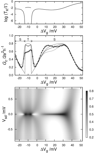
Figure 16: Middle panel: Experimental zero-bias conductance Kogan et al. (2003); foo (c) (crosses) vs $\Delta V_{\mathrm{g}}$ (in $\mathrm{mV}$). Theoretical results obtained as described in text are also shown, for $T/\Gamma=0$ (solid line), $5\times 10^{-3}$ (long dash) and $10^{-2}$ (short dash); for $\Gamma=0.5\mathrm{meV}$ these correspond respectively to $T=0$, $30\mathrm{mK}$ and $60\mathrm{mK}$. The positions of the theoretical phase boundaries ($T=0$) between the USC triplet (T) and Fermi liquid singlet (S) phases are as indicated. Upper panel: Kondo scales determined as in sec. III, and shown as $\log(T_{K}/\Gamma)$ vs $\Delta V_{\mathrm{g}}$ (for the T phase, $T_{K}\equiv T_{K}^{S=1}$). Bottom panel: Theoretical differential conductance map in the ($V_{\mathrm{sd}},\Delta V_{\mathrm{g}}$)-plane, with the grey-scale code indicated (in units of $2e^{2}/h$). Shown for $T=30\mathrm{mK}$, choosing $\Gamma=0.5\mathrm{meV}$ (see text). The experimental counterpart is shown in fig.1 of [Kogan et al., 2003].

Under application of a gate voltage, the level energy $\epsilon_{1}\propto\Delta V_{\mathrm{g}}$, and one expects the level spacing $\Delta\epsilon=\epsilon_{2}-\epsilon_{1}$ to be essentially fixed foo (d). The experimental ‘trajectory’ in the ($\epsilon_{1},\epsilon_{2}$) (or ($x,y$)) plane upon varying $\Delta V_{\mathrm{g}}$ is then as indicated schematically in fig. 2(a), viz. $y=x+\Delta\epsilon$ (i.e. $\epsilon_{2}=\epsilon_{1}+\Delta\epsilon$). In this regard an interesting symmetry arises. Indicating explicitly the $x,y$ dependence of $D_{ee}(\omega)\equiv D_{ee}(\omega;x,y)$, it is readily shown that under the $p$-$h$ and 1-2 transformations of sec. II.1, $D_{ee}(\omega;x,y)=D_{ee}(-\omega;-y,-x)$. Employing this in eqn. (60), noting that $[\partial f_{L}(\omega)/\partial\omega+\partial f_{R}(\omega)/\partial\omega]$ is even in $\omega$, gives

$$G_{c}(T,V_{\mathrm{sd}};x,y)~{}=~{}G_{c}(T,V_{\mathrm{sd}};-y,-x)$$ (62)

for the conductance $G_{c}(T,V_{\mathrm{sd}})\equiv G_{c}(T,V_{\mathrm{sd}};x,y)$. That is, the conductance is symmetric under reflection about the line $y=-x$. Now the ‘trajectory’ $y=x+\Delta\epsilon$ is perpendicular to the line $y=-x$, and intersects it for $x=-\tfrac{1}{2}\Delta\epsilon$, i.e. (since $x=\epsilon_{1}+\tfrac{1}{2}U+U^{\prime}$) for $\epsilon_{1}=-\tfrac{1}{2}\Delta\epsilon-\tfrac{1}{2}U-U^{\prime}\equiv\epsilon_{1,\mathrm{m}}$. Since the phase boundaries are also symmetric under reflection about the line $y=-x$ (figs. (2,5,7)), this value $\epsilon_{1}=\epsilon_{1,\mathrm{m}}$ – and hence the corresponding $\Delta V_{\mathrm{g,m}}$ ($\epsilon_{1}\propto\Delta V_{\mathrm{g}}$) – is thus the midpoint of the triplet phase; such that the conductance should be an even function of $\epsilon_{1}-\epsilon_{1,\mathrm{m}}$, or equivalently of $\Delta V_{\mathrm{g}}-\Delta V_{\mathrm{g,m}}$. This symmetry is quite well satisfied in experiment (and is of course obeyed precisely in the theoretical results). Fig. 16 (middle panel) shows the experimental zero-bias conductance Kogan et al. (2003); foo (c) (crosses) as a function of $\Delta V_{\mathrm{g}}$ (in $\mathrm{mV}$), together with corresponding theoretical results (as detailed below). The midpoint of the triplet (T) phase is readily identified as $\Delta V_{\mathrm{g,m}}=-10~{}\mathrm{mV}$, about which the experimental conductance is indeed seen to be quite symmetric. And the experimental conductance map shown in fig. 1 of [Kogan et al., 2003] (cf fig. 16 bottom panel) is also clearly rather symmetric about $\Delta V_{\mathrm{g,m}}$.

To compare directly to experiment we must specify the dimensionless interactions $\tilde{U},\tilde{U^{\prime}},\tilde{J}_{\mathrm{H}}$ (eqn. (10)), $\Delta\tilde{\epsilon}=\Delta\epsilon/\Gamma$, the relation between $\tilde{\epsilon}_{1}=\epsilon_{1}/\Gamma$ and $\Delta V_{\mathrm{g}}$, and finally the hybridization strength $\Gamma$. This is obviously a large parameter space, and our intent here is simply to employ what we regard as a reasonable set of ‘bare’ parameters. For a typical dot the relative hierarchy of energies satisfies Pustilnik and Glazman (2004) $|\tilde{J}_{\mathrm{H}}|\ll\Delta\tilde{\epsilon}\ll\tilde{U}$; with which the specific parameters we use here concur, $|\tilde{J}_{\mathrm{H}}|=0.5,\Delta\tilde{\epsilon}=4.5$ and $\tilde{U}=12$ (and with $\tilde{U}$ and $\Delta\tilde{\epsilon}$ in excess of unity, consistent with the occurrence of charge quantization towards the centers of the Coulomb blockade valleys). No attempt to explain experiment on the assumption $\tilde{U^{\prime}}=\tilde{U}$ was found to be successful, even qualitatively, on varying the bare parameters. The main reason (as evident from inspection e.g. of fig. 2(c) or fig. 5 (top, (c)) is that the resultant width of the T phase (in $\tilde{\epsilon}_{1}$ or $\Delta V_{\mathrm{g}}$) is much too large compared to that of the singlet (S) phase, and as such not qualitatively consistent with experiment Kogan et al. (2003) (fig. 16). For the results shown here we have used $\tilde{U^{\prime}}=6=\tilde{U}/2$ (although tolerable variations from this value give comparable agreement with experiment).

From the discussion above, the relation between $\Delta V_{\mathrm{g}}$ and $\tilde{\epsilon}_{1}$ is of form $\Delta V_{\mathrm{g}}=c[\tilde{\epsilon}_{1}-\tilde{\epsilon}_{1,\mathrm{m}}]+\Delta V_{\mathrm{g,m}}$ where the proportionality constant $c$ is to be determined (as above, $\Delta V_{\mathrm{g,m}}=-10\mathrm{mV}$ and $\tilde{\epsilon}_{1,\mathrm{m}}=-\tfrac{1}{2}\Delta\tilde{\epsilon}-\tfrac{1}{2}\tilde{U}-\tilde{U^{\prime}}$). For a chosen set of $\tilde{U},\tilde{U^{\prime}},\tilde{J}_{\mathrm{H}},\Delta\tilde{\epsilon}$, the theoretical zero-bias conductance at $T=0$ is calculated from eqn. (59) as a function of $\tilde{\epsilon}_{1}$. It is then scaled onto the experimental results shown in fig. 16 (middle), over the $\Delta V_{\mathrm{g}}$ range above $\sim 35-40\mathrm{mV}$. We choose this range because here the system is beginning the approach to the ‘empty orbital’ regime of $n_{\mathrm{imp}}\ll 1$, where one does not expect any appreciable $T$-dependence to the conductance [the experimental $T$ is not known with certainty foo (c), for although the experiments were performed at the refrigerator base temperature of $\sim 12\mathrm{mK}$, the electron temperature, $T$, was not determined; although it is believed to be $\lesssim 40\mathrm{mK}$ foo (c)]. With this procedure we determine the constant $c$, which is then fixed and used for all $\Delta V_{\mathrm{g}}$ (and $T$); as well as the dimensionless constant $G_{0}$ reflecting (sec. II) the relative asymmetry in tunnel coupling to the leads (from scaling the vertical axis in fig. 16, and leading to $G_{0}\simeq 0.8$ – as is obviously reasonable even from cursory inspection of the experimental data).

In comparing to experiment, an obvious key element is the relative widths (in $\tilde{\epsilon}_{1}$ or $\Delta V_{\mathrm{g}}$) of the S and T phases, the former being considerably wider than the latter in experiment. This we naturally find to be influenced significantly by the exchange $\tilde{J}_{\mathrm{H}}$ (and to a lesser extent by $\Delta\tilde{\epsilon}$), which is optimised accordingly. For the results shown here, we find $\tilde{J}_{\mathrm{H}}=-0.5$ to be optimal. Its magnitude is small, as expected, although its sign is antiferromagnetic. This is not however unreasonable, for on coupling to the leads as mentioned in sec. III, an AF bare $\tilde{J}_{\mathrm{H}}$ still generates an effective ferromagnetic spin-coupling via an RKKY interaction (as evident in the very existence of the USC triplet phase for weakly AF bare $\tilde{J}_{\mathrm{H}}$, and which effect is in fact largest for the case $V_{2}=V_{1}$ we consider explicitly).

With the above we calculate the $T=0$ zero-bias conductance, shown in the middle panel (solid line) of fig. 16 for $\tilde{U}=12,\tilde{U^{\prime}}=6,\Delta\tilde{\epsilon}=4.5,\tilde{J}_{\mathrm{H}}=-0.5$, with the two T/S phase boundaries indicated in the figure. The T phase, symmetrically disposed about the midpoint $\Delta V_{\mathrm{g,m}}=-10\mathrm{mV}$, occurs in the interval $-13.45\mathrm{mV}\leq\Delta V_{\mathrm{g}}\leq-6.55\mathrm{mV}$ (corresponding to $-15.2\leq\tilde{\epsilon}_{1}\leq-13.3$); with $n_{\mathrm{imp}}$ at the phase boundaries of $n_{\mathrm{imp}}=1.87$ (upper boundary at $\Delta V_{\mathrm{g}}=-6.55\mathrm{mV}$) and $n_{\mathrm{imp}}=4-1.87=2.13$ (lower boundary), such that in accordance with eqn. (38) of sec. IV.3 the zero-bias conductance increases on crossing from the S (FL) to the T (USC) phase.

The resultant Kondo scales as a function of $\Delta V_{\mathrm{g}}$ are shown in the top panel of fig. 16 (obtained as specified in sec. III, and with $T_{K}\equiv T_{K}^{S=1}$ for the T phase). Since $T_{K}$ vanishes as the QPT is approached from the S (FL) side, finite-temperature effects will obviously be most significant in the vicinity of the transition. Fig. 16 thus shows the zero-bias conductance at two non-zero temperatures, $T/\Gamma=0.005$ and $0.01$. While there is not much net difference between the two, each has the effect of significantly increasing the conductance in the vicinity of the transition, and leads to what we regard as rather good overall agreement with experiment. Over the $T$-range shown the conductance ‘inside’ the T phase does not erode as rapidly as one might like, reflecting the fact that $T_{K}\equiv T_{K}^{S=1}$ therein is in excess of the $T$’s shown; although one could likely improve on this with a bare parameter set for which $T_{K}^{S=1}$ inside the T phase is somewhat smaller. The temperature range considered here is also entirely reasonable in relation to the experimental $T$ discussed above Kogan et al. (2003); foo (c); with $\Gamma=0.5\mathrm{meV}$ (as employed below) the temperatures shown correspond to $T=30\mathrm{mK}$ and $60\mathrm{mK}$ respectively.

VI.1 Conductance maps

The bare parameters specified above are fixed. Using eqn. (60) the differential conductance, as a function of gate and bias voltages, may now be calculated and compared to experiment. For this we must finally specify the hybridization strength $\Gamma$; in the following we take $\Gamma=0.5\mathrm{meV}$ (noting that comparison to experiment is not critically dependent on this choice, with values in the range $\sim 0.3-0.6\mathrm{meV}$ being found quite acceptable). The resultant differential conductance map for $T=30\mathrm{mK}$ is shown in fig. 16 (bottom panel), and is in rather good agreement with the experimental results reported in fig. 1 of [Kogan et al., 2003].

In addition to the clear zero-bias Kondo ridges associated with both the T and S phases, the conductance map shows other features noted in experiment Kogan et al. (2003). In particular, looking at the far left side of the conductance plot, one sees two dark ‘ridges’ positioned symmetrically around $V_{\mathrm{sd}}=0$. As $\Delta V_{\mathrm{g}}$ is increased the two ridges move together, until they merge to form the zero-bias Kondo ridge associated with the T phase. The latter persists for a range of $\Delta V_{\mathrm{g}}$, and then the two ridges separate again (the pattern being in other words symmetrical about $\Delta V_{\mathrm{g,m}}=-10\mathrm{mV}$, for the reasons explained following eqn. (62)). The obvious question arises as to the origin of these ‘ridges’, which we now consider.

As seen in fig. 16, the $T=0$ zero-bias conductance increases on passing from the S (FL) to the T (USC) phase; and in sec. V.1 we showed that such behavior was indicative of a vanishing Kondo antiresonance in the single-particle spectrum, as the transition is approached from the S side.

Figure 17: Top panel: $V_{\mathrm{sd}}$-dependence of conductance, taking cuts through the conductance map of fig. 16 (bottom) for a sequence of different fixed gate voltages: $\Delta V_{\mathrm{g}}=-10\mathrm{mV}$ (midpoint of the T phase, sold line), and $\Delta V_{\mathrm{g}}/\mathrm{mV}=-6$ (long dash), $-5$ (short dash), $-3$ (point dash) and $+2$ (dotted), on moving into and through the S phase. A clear antiresonance develops in the S phase, as discussed in text. The peaks in the conductance, symmetrical about $V_{\mathrm{sd}}=0$, lie at the center of the ridges seen in the conductance map.
Bottom panel: Focus on the $\Delta V_{\mathrm{g}}=-3\mathrm{mV}$ case. Solid line: conductance as in top panel. Long dash: corresponding $T=0$ conductance, proportional to $[D_{ee}(\omega=+\tfrac{1}{2}eV_{\mathrm{sd}})+D_{ee}(\omega=-\tfrac{1}{2}eV_{\mathrm{sd}})]$. Short dash: contribution from $D_{ee}(\omega=+\tfrac{1}{2}eV_{\mathrm{sd}})$ alone, showing a clear Kondo antiresonance in the single-particle spectrum itself.

This is the origin of the ridges seen in the conductance maps, as now shown by considering cuts through the conductance map of fig. 16, for a sequence of different fixed gate voltages $\Delta V_{\mathrm{g}}$. The top panel in fig. 17 accordingly shows the conductance vs bias voltage $V_{\mathrm{sd}}$, for five different values of $\Delta V_{\mathrm{g}}$: $-10\mathrm{mV}$ (at the midpoint of the T phase), and $\Delta V_{\mathrm{g}}=-6,-5,-3$ and $+2$ $\mathrm{mV}$ as one moves into the S phase (which at $T=0$ occurs for $\Delta V_{\mathrm{g}}\geq-6.5\mathrm{mV}$). For $\Delta V_{\mathrm{g}}=-10\mathrm{mV}$ the conductance naturally peaks at $V_{\mathrm{sd}}=0$. But on entering the S phase a clear antiresonance in the conductance is seen to develop, just setting in by $\Delta V_{\mathrm{g}}=-6\mathrm{mV}$ and deepening progressively as $\Delta V_{\mathrm{g}}$ is increased in the S phase towards $-3\mathrm{mV}$ (then naturally disappearing as one gets considerably further into the S phase, as illustrated by the $\Delta V_{\mathrm{g}}=+2\mathrm{mV}$ example). And the peaks in these conductance profiles, symmetrically disposed about $V_{\mathrm{sd}}=0$, lie at the center of the ridges in the conductance map.

To show that the above behavior indeed reflects a Kondo antiresonance in the single-particle spectrum itself, the bottom panel in fig. 17 focusses on the $\Delta V_{\mathrm{g}}=-3\mathrm{mV}$ example. The solid line again gives the conductance shown in the top panel; while the long dash line shows the corresponding $T=0$ conductance obtained from eqn. (61), and thus being proportional to $[D_{ee}(\omega=+\tfrac{1}{2}eV_{\mathrm{sd}})+D_{ee}(\omega=-\tfrac{1}{2}eV_{\mathrm{sd}})]$. The latter clearly captures well the former (the differences naturally being due to thermal smearing). Because the conductance is proportional to the symmetrized spectra at $\omega=\pm\tfrac{1}{2}eV_{\mathrm{sd}}$, it is not a priori clear that the single-particle spectrum itself contains a Kondo antiresonance. That it does, however, is seen from short-dash line in fig. 17(bottom), which shows the contribution from $D_{ee}(\omega=+\tfrac{1}{2}eV_{\mathrm{sd}})$ itself, seen to contain a clear Kondo antiresonance centered on the Fermi level. We add too that, since the peaks/ridges in the conductance stem from the ‘peaks’ inherent to the Kondo antiresonance in $D_{ee}$, they are obviously not interpretable in terms of isolated dot states.

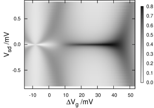
Figure 18: As discussed in text, differential conductance map in the ($V_{\mathrm{sd}},\Delta V_{\mathrm{g}}$)-plane; shown for $T=30\mathrm{mK}$ with the same bare parameters as figs. (16,17), except for a slight change in $\tilde{J}_{\mathrm{H}}$. In this case no S/T transition occurs, the system remaining throughout in the S phase. The zero-bias Kondo ridge associated with the T phase is thus absent, and instead a zero-bias conductance antiresonance persists.

Finally, the zero-bias Kondo ridge in the conductance map – formed as described above on merging of the $V_{\mathrm{sd}}\neq 0$ conductance ridges, and concomitant vanishing of a conductance antiresonance (as in fig. 17 top) – reflects of course the existence of the T (USC) phase, and hence a transition to it from the S (FL) phase. However one can readily envisage a situation where the underlying bare parameters of the system/device are slightly different, such that on ramping down the gate voltage the resultant trajectory $y=x+\Delta\epsilon$ comes close to but ‘misses’ the S/T transition; the system as such always remaining in a S phase (see e.g. fig. 2(a)). In this case no zero-bias Kondo ridge associated with the T phase can arise. Instead, from the discussion above, one might intuitively expect continued persistence of the conductance antiresonance on decreasing $\Delta V_{\mathrm{g}}$, with attendant finite-bias conductance ridges which never quite merge together. That this indeed occurs is illustrated in fig. 18, where the conductance map (here for $T=30\mathrm{mK}$) is shown for the same bare parameters as figs. (16,17), except for a slight change in $\tilde{J}_{\mathrm{H}}$ to $-0.6$ (the same behavior arising also on changing e.g. $\Delta\tilde{\epsilon}$ rather than $\tilde{J}_{\mathrm{H}}$). And the qualitative behavior seen here is indeed similar to that observed in a second device, shown in fig. 3 of [Kogan et al., 2003] (although in this case we have not made a quantitative comparison).

VII Concluding remarks

As exemplars of multilevel quantum dot systems, we have considered in this paper correlated two-level quantum dots, coupled in a 1-channel fashion to metallic leads. Thermodynamics, single-particle dynamics and electronic transport properties show the physical behavior of the system to be rich and varied; and our aim has been to obtain a unified understanding of the problem for essentially arbitrary dot charge/occupancy. Excepting points of high symmetry where first order level-crossing transitions arise, associated quantum phase transitions are of Kosterlitz-Thouless type, evident in a vanishing Kondo scale as the transition to the underscreened spin-1 phase is approached from the Fermi liquid side; and manifest in particular by a discontinuous jump in the zero-bias conductance as the transition is crossed, which we have shown can be understood here from an underlying Friedel-Luttinger sum rule. We add in fact that an abrupt conductance change appears to be a general signature of a KT transition, such behavior arising generally not only in the present model, but also in capacitively coupled 2-channel quantum dots which exhibit a KT transition from a charge-Kondo Fermi liquid state (with a quenched charge pseudospin) to a non-Fermi liquid, doubly degenerate ‘charge-ordered’ phase Galpin et al. (2005); and in the problem of spinless, capacitively coupled metallic islands/large dots close to a degeneracy point between $N$ and $N+1$ electron states, described by two Ising-coupled Kondo impurities Garst et al. (2004).

Several issues naturally remain to be addressed. We believe for example that the generalization of Luttinger’s theorem to the singular Fermi liquid USC phase (sec. IV.2) is significant, and raises important basic questions (such as why, and what fundamentally does it reflect?). While we do not doubt its validity, we have however demonstrated it only numerically; and a proper analytical understanding of the result is obviously desirable. In this work we have also considered the system in the absence of an applied magnetic field, $B$. Interesting physics arises also for $B\neq 0$ (see e.g. [Pustilnik and Borda, 2006]), where the underlying quantum phase transitions are naturally smeared into crossovers. In fact, for the USC phase the limits of zero field and $B\rightarrow 0+$ are different for $T=0$, reflecting the total polarization of a free spin-1/2 (as for the USC fixed point) on application of even an infinitesimal field. We will turn in subsequent work to the effects of magnetic fields upon single-particle dynamics and transport in the model.

Appendix A Effective low-energy models

We first sketch the derivation of the effective low-energy model considered in sec. III.2, spanned by the ($1,1$) triplet and ($1,1$) singlet states of the isolated dot; with energies under $\hat{H}_{\mathrm{D}}$ of $E_{T}=\epsilon_{1}+\epsilon_{2}+U^{\prime}-\tfrac{1}{4}J_{\mathrm{H}}$ and $E_{S}=\epsilon_{1}+\epsilon_{2}+U^{\prime}+\tfrac{3}{4}J_{\mathrm{H}}$ respectively. The local unity operator for the dot is

$$\hat{1}~{}=~{}\hat{1}_{\mathrm{T}}~{}+~{}\hat{1}_{\mathrm{S}}$$ (63)

with $\hat{1}_{\mathrm{T}}=\sum_{S^{z}}~{}|S=1,S^{z}\rangle\langle S=1,S^{z}|$ in an obvious notation, and likewise $\hat{1}_{\mathrm{S}}=|0,0\rangle\langle 0,0|$. These satisfy the following identities in the local Hilbert space,

$$\hat{1}_{\mathrm{T}}~{}=~{}~{}\hat{\mathbf{s}}_{1}\cdot\hat{\mathbf{s}}_{2}~{}+~{}\tfrac{3}{4}\hat{1}~{}~{}~{}~{}~{}~{}~{}~{}~{}~{}\hat{1}_{\mathrm{S}}~{}=~{}-\hat{\mathbf{s}}_{1}\cdot\hat{\mathbf{s}}_{2}~{}+~{}\tfrac{1}{4}\hat{1},$$ (64)

as follows using $\hat{\mathbf{s}}_{1}\cdot\hat{\mathbf{s}}_{2}\equiv\tfrac{1}{2}\left(\hat{S}^{2}-\tfrac{3}{2}\right)$ with $\hat{\mathbf{S}}=\hat{\mathbf{s}}_{1}+\hat{\mathbf{s}}_{2}$.

Omitting for brevity the lead contribution $\hat{H}_{\mathrm{L}}$ (eqn. (3)), the low-energy model is given by $\hat{H}_{\mathrm{eff}}=E_{S}\hat{1}_{\mathrm{S}}+E_{T}\hat{1}_{\mathrm{T}}+\hat{H}^{(2)}_{\mathrm{eff}}$. The first two terms are simply the bare energies of the dot states; using eqns. (63,64) they may be written as $E_{S}\hat{1}_{\mathrm{S}}+E_{T}\hat{1}_{\mathrm{T}}=\tfrac{1}{4}(E_{S}+3E_{T})\hat{1}+(E_{T}-E_{S})\hat{\mathbf{s}}_{1}\cdot\hat{\mathbf{s}}_{2}$, or equivalently as $-J_{\mathrm{H}}\hat{\mathbf{s}}_{1}\cdot\hat{\mathbf{s}}_{2}$ on omitting the first (constant/common) term:

$$\hat{H}_{\mathrm{eff}}~{}=~{}-J_{\mathrm{H}}\hat{\mathbf{s}}_{1}\cdot\hat{\mathbf{s}}_{2}~{}+~{}\hat{H}^{(2)}_{\mathrm{eff}}$$ (65)

Here $\hat{H}^{(2)}_{\mathrm{eff}}$ is the leading (${\cal{O}}(V^{2})$) contribution arising from tunnel coupling to the leads (eqn. (2) with $V_{2}=V_{1}\equiv V$, here denoted as $\hat{H}^{\prime}$), given from a SW transformation Schrieffer and Wolff (1966) as

$$\hat{H}^{(2)}_{\mathrm{eff}}=\tfrac{1}{2}\sum_{\alpha,\beta}~{}\hat{1}_{\beta}\hat{H}^{\prime}\left[\left(E_{\alpha}-\hat{H}_{D}\right)^{-1}+\left(E_{\beta}-\hat{H}_{D}\right)^{-1}\right]\hat{H}^{\prime}\hat{1}_{\alpha}$$ (66)

with $\alpha,\beta\in\{S,T\}$ (retardation effects are as usual neglected).

In analyzing eqn. (66) one encounters the following ‘natural’ exchange couplings $J_{i}^{\alpha}>0$,

$$J_{i}^{\alpha}~{}=~{}NV^{2}\left[\frac{1}{\Delta E_{i}^{\alpha}}+\frac{1}{\Delta\tilde{E}_{i}^{\alpha}}\right]$$ (67)

(with $N$ the number of $\mathbf{k}$-states in the lead, such that $NV^{2}\sim{\cal{O}}(1)$). Here the $\Delta E_{i}^{\alpha}>0$ denote electron removal excitation energies from level $i=1$ or $2$, relative to the $\alpha=T$ or $S$ dot ground state, and the $\Delta\tilde{E}_{i}^{\alpha}>0$ correspondingly denote electron addition energies to level $i$ relative to the $\alpha=T$ or $S$ ground state; e.g. $\Delta E^{T}_{1}=E_{D}(0,1)-E_{T}$ or $\Delta\tilde{E}^{S}_{2}=E_{D}(1,2)-E_{S}$ in the notation of sec. II.2. Denoting

$$\lambda_{T}=\tfrac{1}{2}U+\tfrac{1}{4}J_{\mathrm{H}}~{}~{}~{}~{}~{}~{}~{}~{}\lambda_{S}=\tfrac{1}{2}U-\tfrac{3}{4}J_{\mathrm{H}}$$ (68)

these excitation energies are easily shown to be given by

$$\Delta E_{1}^{\alpha}=\lambda_{\alpha}-x~{}~{}~{}~{}~{}~{}~{}~{}~{}\Delta\tilde{E}_{1}^{\alpha}=\lambda_{\alpha}+x$$ (69a)

$$\Delta E_{2}^{\alpha}=\lambda_{\alpha}-y~{}~{}~{}~{}~{}~{}~{}~{}~{}\Delta\tilde{E}_{2}^{\alpha}=\lambda_{\alpha}+y$$ (69b)

where (eqn. (11)) $x=\epsilon_{1}+\tfrac{1}{2}U+U^{\prime}$, $y=\epsilon_{2}+\tfrac{1}{2}U+U^{\prime}$. Hence from eqn. (67),

$$J_{1}^{\alpha}\equiv J^{\alpha}(x)~{}~{}~{}~{}~{}~{}~{}~{}J_{2}^{\alpha}\equiv J^{\alpha}(y)$$ (70)

with $J^{\alpha}(x)$ defined by:

$$J^{\alpha}(x)~{}=~{}NV^{2}\left[\frac{1}{\lambda_{\alpha}-x}~{}+~{}\frac{1}{\lambda_{\alpha}+x}\right]~{}~{}~{}~{}=~{}J^{\alpha}(-x)$$ (71)

Direct analysis of eqn. (66) yields, after a standard if laborious calculation, the effective low-energy model eqn. (16),

$$\hat{H}_{\mathrm{eff}}~{}=~{}J_{1}(x,y)~{}\hat{\mathbf{s}}_{1}\cdot\hat{\mathbf{s}}_{0}~{}+~{}J_{2}(x,y)~{}\hat{\mathbf{s}}_{2}\cdot\hat{\mathbf{s}}_{0}~{}-~{}I(x,y)~{}\hat{\mathbf{s}}_{1}\cdot\hat{\mathbf{s}}_{2}$$ (72)

where potential scattering contributions are omitted for clarity, and $\hat{\mathbf{s}}_{0}$ denotes the spin density of the conduction channel at the dot. The direct exchange coupling between spins $1$ and $2$ is found to be

$$I(x,y)~{}=~{}J_{\mathrm{H}}~{}+~{}\tfrac{1}{2}\left[J^{T}(x)+J^{T}(y)-J^{S}(x)-J^{S}(y)\right]$$ (73)

while the ${\cal{O}}(V^{2})$ antiferromagnetic exchange couplings between spins $1$ or $2$ and the lead are given by

$$J_{1}(x,y)~{}=~{}\tfrac{1}{2}\left[3J^{T}(x)+J^{T}(y)+\left(J^{S}(x)-J^{S}(y)\right)\right]$$ (74a)

$$J_{2}(x,y)~{}=~{}J_{1}(y,x).$$ (74b)

Using eqn. (71), these exchange couplings satisfy

$$J_{i}(x,y)~{}=~{}J_{i}(-x,-y)~{}~{}~{}~{}~{}~{}~{}~{}:i=1,2$$ (75a)

$$I(x,y)~{}~{}=~{}~{}I(-x,-y)~{}~{}=~{}~{}I(y,x)~{}~{}~{}~{}$$ (75b)

by virtue of which $\hat{H}_{\mathrm{eff}}\equiv\hat{H}_{\mathrm{eff}}(x,y)$ in eqn. (72) satisfies $\hat{H}_{\mathrm{eff}}(x,y)\equiv\hat{H}_{\mathrm{eff}}(-x,-y)$ (reflecting its symmetry under a $p$-$h$ transformation); while from eqn. (74b), $\hat{H}_{\mathrm{eff}}(x,y)\rightarrow\hat{H}_{\mathrm{eff}}(y,x)$ under the 1-2 transformation (eqn. (13)), as expected on general grounds from sec. II.1. These symmetries, and the consequent invariance of the phase boundaries in the ($x,y$)-plane to both inversion and reflection about the line $y=x$, are also naturally satisfied when potential scattering terms, omitted explicitly from eqn. (72), are included. By contrast, the apparent reflection symmetries $\hat{H}_{\mathrm{eff}}(x,y)=\hat{H}_{\mathrm{eff}}(-x,y)=\hat{H}_{\mathrm{eff}}(x,-y)$ which hold for eqn. (72) itself (via eqn. (71)), are not preserved when potential scattering is included; which is why the phase boundaries in fig. 7 are not invariant to reflection about the lines $x=0$ and $y=0$.

Along the lines $y=\pm x$ in the ($x,y$)-plane, it follows directly from eqns. (74b,75a) that $J_{2}(x,\pm x)=J_{1}(x,\pm x)$, and hence from eqns. (74a,71)

$$J_{2}(x,\pm x)~{}=~{}J_{1}(x,\pm x)~{}=~{}2J^{T}(x),$$ (76)

with $I(x,\pm x)=J_{\mathrm{H}}+[J^{T}(x)-J^{S}(x)]$ following similarly from eqn. (73). In consequence, as discussed in sec. III.2, $\hat{H}_{\mathrm{eff}}$ is separable along the lines $y=\pm x$, and first order level-crossing transitions thus arise. Note incidentally that for given $J_{\mathrm{H}}<0$, both $J^{T}(x)$ and $I(x,\pm x)$ increase on increasing $|x|$ from $0$, both of which act (see eqn. (17)) to favor the triplet phase; consistent with the USC phase surviving for $|x|>0$ after it has been destroyed for $x=0$, as indeed found in fig. 7.

Finally, a byproduct of the above gives directly the pure spin-1 Kondo model appropriate for ferromagnetic $J_{\mathrm{H}}>0$ deep in the USC spin-1 phase Pustilnik and Glazman (2001); Posazhennikova et al. (2007), where the ($1,1$) singlet dot states are energetically irrelevant and only the $(1,1)$ triplet states need be retained. To this end simply project into the triplet sector, $\hat{H}_{K}=\hat{1}_{\mathrm{T}}\hat{H}_{\mathrm{eff}}\hat{1}_{\mathrm{T}}$. Writing $J_{1}\hat{\mathbf{s}}_{1}\cdot\hat{\mathbf{s}}_{0}+J_{2}\hat{\mathbf{s}}_{2}\cdot\hat{\mathbf{s}}_{0}=$ $\tfrac{1}{2}(J_{1}+J_{2})(\hat{\mathbf{s}}_{1}+\hat{\mathbf{s}}_{2})\cdot\hat{\mathbf{s}}_{0}$ $+\tfrac{1}{2}(J_{1}-J_{2})(\hat{\mathbf{s}}_{1}-\hat{\mathbf{s}}_{2})\cdot\hat{\mathbf{s}}_{0}$, recognising that $\hat{1}_{\mathrm{T}}(\hat{\mathbf{s}}_{1}-\hat{\mathbf{s}}_{2})\hat{1}_{\mathrm{T}}=0$ and neglecting constants, eqn. (72) gives a spin-1 Kondo model

$$\hat{H}_{K}~{}=~{}\hat{1}_{\mathrm{T}}\hat{H}_{\mathrm{eff}}\hat{1}_{\mathrm{T}}~{}=~{}J_{K}~{}\hat{\mathbf{S}}\cdot\hat{\mathbf{s}}_{0}$$ (77)

where $\hat{\mathbf{S}}\equiv\hat{1}_{\mathrm{T}}(\hat{\mathbf{s}}_{1}+\hat{\mathbf{s}}_{2})\hat{1}_{\mathrm{T}}$ is a pure spin-1 operator, and $J_{K}=\tfrac{1}{2}(J_{1}+J_{2})$ is given from eqn. (74) by

$$J_{K}~{}=~{}J^{T}(x)+J^{T}(y)$$ (78)

with $J^{T}(x)$ given explicitly by eqn. (71). Along the lines $y=\pm x$ in particular, eqns. (78,71,68) give $J_{K}=2J^{T}(x)$; i.e. $\rho J_{K}=\tfrac{8}{\pi}\Gamma[U+\tfrac{1}{2}J_{\mathrm{H}}]/([U+\tfrac{1}{2}J_{\mathrm{H}}]^{2}-x^{2})$ with $\rho$ here the lead density of states per conduction orbital (such that $\Gamma\equiv\pi V^{2}N\rho$). From perturbative scaling Hewson (1993) the spin-1 Kondo scale $T_{K}^{S=1}$ follows as $T_{K}^{S=1}\sim D\exp(-1/\rho J_{K})$ (with the exponential dependence as usual of the essence, and the prefactor immaterial), and eqn. (42) for $T_{K}^{S=1}$ thus results. From NRG calculations we have confirmed explicitly that the dependence of $T_{K}^{S=1}$ on $\tilde{U}+\tfrac{1}{2}\tilde{J}_{\mathrm{H}}$ is indeed as predicted by eqn. (42).

Appendix B Self-energies

The key NRG method for calculating the self-energy Bulla et al. (1998) is readily extended to multilevel dots/impurities. With $\hat{H}_{I}$ the interacting part of the dot Hamiltonian, equation of motion techniques Zubarev (1960) are used to obtain the following basic equation for the retarded propagators $\{G_{ij}(\omega)\}$:

$$\sum_{l}\left((\omega^{+}-\epsilon_{i})\delta_{il}-\Gamma_{il}(\omega)\right)G_{lj}(\omega)~{}=~{}\delta_{ij}+\langle\langle[d^{\phantom{\dagger}}_{i\sigma},\hat{H}_{I}^{\phantom{\dagger}}];d_{j\sigma}^{\dagger}\rangle\rangle$$ (79)

The sum is over the dot levels ($l=1,2$ here), and $[,]$ denotes a commutator. By definition, $\hat{H}_{I}\equiv 0$ in the non-interacting limit; whence eqn. (79) is of form

$$\left[\bm{G}^{0}(\omega)\right]^{-1}\bm{G}(\omega)~{}=~{}\bm{1}+\bm{F}(\omega)$$ (80)

with $\bm{G}^{0}(\omega)$ the non-interacting propagator matrix and the elements of $\bm{F}(\omega)$ given by:

$$F_{ij}(\omega)~{}=~{}\langle\langle~{}[d^{\phantom{\dagger}}_{i\sigma},\hat{H}_{I}^{\phantom{\dagger}}];d^{\dagger}_{j\sigma}~{}\rangle\rangle$$ (81)

Using the Dyson equation in the form $[\bm{G}^{0}]^{-1}=[\bm{G}]^{-1}+\bm{\Sigma}$, eqn. (80) gives directly eqn. (39),

$$\bm{\Sigma}(\omega)~{}=~{}\bm{F}(\omega)[\bm{G}(\omega)]^{-1}$$ (82)

from which the self-energies are calculated directly (sec. V). Combining eqn. (82) with the Dyson equation also gives $\bm{G}=\bm{G}^{0}(\bm{1}+\bm{F})$, so that eqn. (82) may be written alternatively as

$$\bm{\Sigma}(\omega)~{}=~{}\bm{F}(\omega)\left[\bm{1}+\bm{F}(\omega)\right]^{-1}\left[\bm{G}^{0}(\omega)\right]^{-1}$$ (83)

(which we exploit to calculate the renormalized level $\epsilon_{o}^{*}$ when considering dynamics on the $y=x$ line, eqn. (54) sec. V.2).

$\hat{H}_{I}$ is given explicitly for the present problem by the separable sum (eqn. (1)) $\hat{H}_{I}=U\sum_{i}\hat{n}_{i\uparrow}^{\phantom{\dagger}}\hat{n}_{i\downarrow}^{\phantom{\dagger}}+U^{\prime}\hat{n}_{1}^{\phantom{\dagger}}\hat{n}_{2}^{\phantom{\dagger}}-J_{\mathrm{H}}~{}\hat{\mathbf{s}}_{1}\cdot\hat{\mathbf{s}}_{2}$. The elements eqn. (81) of $\bm{F}$ are thus linearly separable as $F_{ij}=F_{ij}^{U}+F_{ij}^{U^{\prime}}+F_{ij}^{J}$ (in obvious notation), and are calculated individually. Since each such term is a retarded correlation function, they are Lehmann resolvable Abrikosov et al. (1977), and in consequence satisfy sum rules. Writing $F_{ij}(\omega)=F_{ij}^{R}(\omega)-\mathrm{i}F_{ij}^{I}(\omega)$ (with the real/imaginary parts related by Hilbert transformation), the general sum rule is

$$\int^{\infty}_{-\infty}\frac{d\omega}{\pi}~{}F_{ij}^{I}(\omega)~{}=~{}\langle\big{\{}[d^{\phantom{\dagger}}_{i\sigma},\hat{H}_{I}],d_{j\sigma}^{\dagger}\big{\}}\rangle$$ (84)

where $\{,\}$ denotes an anticommutator. Specifically, for the present problem in the absence of an applied magnetic field, it is readily shown that the diagonal-element sum rule is

$$\int^{\infty}_{-\infty}\frac{d\omega}{\pi}~{}F_{ii}^{I}(\omega)~{}=~{}\tfrac{1}{2}U\langle\hat{n}_{i}^{\phantom{\dagger}}\rangle~{}+~{}U^{\prime}\langle\hat{n}^{\phantom{\dagger}}_{\bar{i}}\rangle$$ (85)

(where $\bar{i}$ means the opposite level to $i$); while for the off-diagonal elements:

$$\int^{\infty}_{-\infty}\frac{d\omega}{\pi}~{}F_{ij}^{I}(\omega)~{} \overset{j\neq i}{=}~{}\left(-U^{\prime}+\tfrac{3}{4}J_{\mathrm{H}}\right)\langle d^{\dagger}_{j\sigma}d^{\phantom{\dagger}}_{i\sigma}\rangle$$ (86a)

$$=~{}\left(-U^{\prime}+\tfrac{3}{4}J_{\mathrm{H}}\right)\int^{0}_{-\infty}d\omega~{}D_{ij}(\omega)~{}~{}~{}~{}~{}$$ (86b)

These sum rules provide a check on the accuracy of the NRG calculations, and in practice are well satisfied.

References

- Hewson (1993) A. C. Hewson, The Kondo Problem to Heavy Fermions (Cambridge University Press, Cambridge, 1993).
- Kouwenhoven et al. (1997) L. P. Kouwenhoven et al., in Mesoscopic Electron Transport, edited by L. L. Sohn (Kluwer, Dordrecht, 1997).
- Pustilnik and Glazman (2004) M. Pustilnik and L. I. Glazman, J. Phys.: Condens. Matter 16, R513 (2004).
- Goldhaber-Gordon et al. (1998) D. Goldhaber-Gordon, H. Shtrikman, D. Mahalu, D. Abusch-Magder, U. Meirav, and M. A. Kastner, Nature 391, 156 (1998).
- Cronenwett et al. (1998) S. M. Cronenwett, T. H. Oosterkamp, and L. P. Kouwenhoven, Science 281, 540 (1998).
- Anderson (1961) P. W. Anderson, Phys. Rev. 124, 41 (1961).
- Brouwer et al. (1999) P. W. Brouwer, Y. Oreg, and B. I. Halperin, Phys. Rev. B 60, R13977 (1999).
- Baranger et al. (2000) H. U. Baranger, D. Ullmo, and L. I. Glazman, Phys. Rev. B 61, R2425 (2000).
- Schmid et al. (2000) J. Schmid, J. Weis, K. Eberl, and K. v Klitzing, Phys. Rev. Lett. 84, 5824 (2000).
- van der Wiel et al. (2002) W. G. van der Wiel, S. De Franceschi, J. M. Elzerman, S. Tarucha, L. P. Kouwenhoven, J. Motohisa, F. Nakajima, and T. Fukui, Phys. Rev. Lett. 88, 126803 (2002).
- Kogan et al. (2003) A. Kogan, G. Granger, M. A. Kastner, D. Goldhaber-Gordon, and H. Shtrikman, Phys. Rev. B 67, 113309 (2003).
- Quay et al. (2007) C. H. L. Quay, J. Cumings, S. J. Gamble, R. de Picciotto, H. Kataura, and D. Goldhaber-Gordon, Phys. Rev. B 76, 245311 (2007).
- Sasaki et al. (2000) S. Sasaki, S. De Franceschi, J. M. Elzerman, W. G. van der Wiel, M. Eto, S. Tarucha, and L. P. Kouwenhoven, Nature 405, 764 (2000).
- Roch et al. (2008) N. Roch, S. Florens, V. Bouchiat, W. Wernsdorfer, and F. Balestro, Nature 453, 633 (2008).
- Pustilnik and Glazman (2001) M. Pustilnik and L. I. Glazman, Phys. Rev. Lett. 87, 216601 (2001).
- Posazhennikova et al. (2007) A. Posazhennikova, B. Bayani, and P. Coleman, Phys. Rev. B 75, 245329 (2007).
- Nozières and Blandin (1980) P. Nozières and A. Blandin, J. de Phys. (France) 41, 193 (1980).
- Kikoin and Avishai (2001) K. Kikoin and Y. Avishai, Phys. Rev. Lett. 86, 2090 (2001).
- Hofstetter and Schoeller (2001) W. Hofstetter and H. Schoeller, Phys. Rev. Lett. 88, 016803 (2001).
- Vojta et al. (2002) M. Vojta, R. Bulla, and W. Hofstetter, Phys. Rev. B 65, 140405(R) (2002).
- Koller et al. (2005) W. Koller, A. C. Hewson, and D. Meyer, Phys. Rev. B 72, 045117 (2005).
- Pustilnik and Borda (2006) M. Pustilnik and L. Borda, Phys. Rev. B 73, 201301(R) (2006).
- Posazhennikova and Coleman (2005) A. Posazhennikova and P. Coleman, Phys. Rev. Lett. 94, 036802 (2005).
- Bas and Aligia (2009) P. R. Bas and A. A. Aligia, cond-mat/09043236 (2009).
- Pustilnik and Glazman (2000) M. Pustilnik and L. I. Glazman, Phys. Rev. Lett. 85, 2993 (2000).
- Pustilnik et al. (2003) M. Pustilnik, L. I. Glazman, and W. Hofstetter, Phys. Rev. B 68, 161303(R) (2003).
- Hofstetter and Zarand (2004) W. Hofstetter and G. Zarand, Phys. Rev. B 69, 235301 (2004).
- Mehta et al. (2005) P. Mehta, N. Andrei, P. Coleman, L. Borda, and G. Zarand, Phys. Rev. B 72, 014430 (2005).
- Wilson (1975) K. G. Wilson, Rev. Mod. Phys. 47, 773 (1975).
- Krishnamurthy et al. (1980a) H. R. Krishnamurthy, J. W. Wilkins, and K. G. Wilson, Phys. Rev. B 21, 1003 (1980a).
- Krishnamurthy et al. (1980b) H. R. Krishnamurthy, J. W. Wilkins, and K. G. Wilson, Phys. Rev. B 21, 1044 (1980b).
- Peters et al. (2006) R. Peters, T. Pruschke, and F. B. Anders, Phys. Rev. B 74, 245114 (2006).
- Weichselbaum and von Delft (2007) A. Weichselbaum and J. von Delft, Phys. Rev. Lett. 99, 076402 (2007).
- Bulla et al. (2008) R. Bulla, T. Costi, and T. Pruschke, Rev. Mod. Phys. 80, 395 (2008).
- Langreth (1966) D. C. Langreth, Phys. Rev. 150, 516 (1966).
- Luttinger (1960) J. M. Luttinger, Phys. Rev. 119, 1153 (1960).
- Meir and Wingreen (1992) Y. Meir and N. S. Wingreen, Phys. Rev. Lett. 68, 2512 (1992).
- Schrieffer and Wolff (1966) J. R. Schrieffer and P. A. Wolff, Phys. Rev. 149, 491 (1966).
- Mitchell et al. (2009) A. K. Mitchell, T. F. Jarrold, and D. E. Logan, Phys. Rev. B 79, 085124 (2009).
- foo (a) In practice we define the low-energy scale via , suitably between and .
- foo (b) The reader will notice from fig. 7 that the first order transitions along occur on the ‘inside’ intersection of this line with the phase boundary, but not on the outer intersection. This reflects the fact that eqn. (16) itself is not in fact applicable in the latter region, constructed as it is retaining solely the () singlet and triplet states of the dot. On progressively increasing along the line , the () (or ()) singlet states of the dot must also be retained in the low-energy manifold, leading to a different effective low-energy model with a non-separable Hilbert space.
- Zubarev (1960) D. N. Zubarev, Sov. Phys. Usp. 3, 320 (1960).
- Bulla et al. (1998) R. Bulla, A. C. Hewson, and T. Pruschke, J. Phys.: Condens. Matter 10, 8365 (1998).
- Abrikosov et al. (1977) A. A. Abrikosov, L. P. Gorkov, and I. E. Dzyaloshinski, Methods of Quantum Field Theory in Statistical Physics (Dover, New York, 1977).
- Oliveira and Oliveira (1994) W. C. Oliveira and L. N. Oliveira, Phys. Rev. B 49, 11986 (1994).
- foo (c) A. Kogan and D. Goldhaber-Gordon, private communication.
- foo (d) Any variation of with is a much weaker effect and thus usually neglected. We can in principle include it, but in comparing to experiment here do not find it necessary to do so.
- Galpin et al. (2005) M. R. Galpin, D. E. Logan, and H. R. Krishnamurthy, Phys. Rev. Lett. 94, 186406 (2005).
- Garst et al. (2004) M. Garst, S. Kehrein, T. Pruschke, A. Rosch, and M. Vojta, Phys. Rev. B 69, 214413 (2004).