Constraints on opacities from complex asteroseismology of B-type pulsators: the $\beta$ Cephei star $\theta$ Ophiuchi

Abstract

We present results of a comprehensive asteroseismic modelling of the $\beta$ Cephei variable $\theta$ Ophiuchi. We call these studies complex asteroseismology because our goal is to reproduce both pulsational frequencies as well as corresponding values of a complex, nonadiabatic parameter, $f$, defined by the radiative flux perturbation. To this end, we apply the method of simultaneous determination of the spherical harmonic degree, $\ell$, of excited pulsational mode and the corresponding nonadiabatic $f$ parameter from combined multicolour photometry and radial velocity data. Using both the OP and OPAL opacity data, we find a family of seismic models which reproduce the radial and dipole centroid mode frequencies, as well as the $f$ parameter associated with the radial mode. Adding the nonadiabatic parameter to seismic modelling of the B-type main sequence pulsators yields very strong constraints on stellar opacities. In particular, only with one source of opacities it is possible to agree the empirical values of $f$ with their theoretical counterparts. Our results for $\theta$ Oph point substantially to preference for the OPAL data.

1 Introduction

During the last two decades, $\beta$ Cephei stars became attractive targets for asteroseismic studies. This has started with the pioneering papers by Dziembowski & Jerzykiewicz on 16 Lac and 12 Lac (Dziembowski & Jerzykiewicz, 1996 and 1999, respectively). The analysis of multiplets in 16 Lac showed that rotation rate of this star has to increase inward. The seismic modelling of B-type pulsators have been revived with the paper by Aerts, Toul, Daszyńska et al. (2003) on V836 Cen, in which they also found a non-rigid rotation and, for the first time, an evidence for overshooting from a convective core in a massive main sequence star. Up to now, the most intensively studied $\beta$ Cephei stars have been $\nu$ Eri and 12 Lac which were subjects of multi-site photometric and spectroscopic campaigns (Handler et al. 2004, Aerts et al. 2004, Jerzykiewicz et al. 2005, Handler et al. 2006). The seismic modelling of $\nu$ Eri was done by Pamyatnykh, Handler & Dziembowski (2004) and Ausseloos et al. (2004). Stronger constraints on stellar structure can be obtained from asteroseismology of the hybrid B-type pulsators in which two types of modes are excited simultaneously, i.e., low-order pressure and gravity modes (typical for $\beta$ Cephei stars) and high-order gravity modes (typical for Slowly Pulsating B-type stars). Such studies were done recently by Dziembowski & Pamyatnykh (2008) for $\nu$ Eri and 12 Lac. Interesting results are coming up for another hybrid pulsating star $\gamma$ Peg (Handler et al. 2009).

Until now, asteroseismic studies have relied on fitting only pulsation frequencies. The ultimate goal has been to find models which reproduce observed frequencies by changing various parameters of model and theory, provided that the successful mode identification was obtained beforehand. However oscillation frequencies are determined mainly by the star’s interior, thus they are rather weakly sensitive to the subphotospheric layers. A few years ago, Daszyńska-Daszkiewicz, Dziembowski & Pamyatnykh (2003 and 2005a, hereafter DD03 and DD05) introduced a new asteroseismic probe, defined as the ratio of the amplitude of the bolometric flux variations to the radial displacement at the photosphere level. This is so called $f$ parameter; it is determined in the pulsation driving region.

The $f$ parameter exhibits a strong dependence on the global stellar parameters, chemical composition, opacities and subphotospheric convection. Therefore, a comparison of empirical values of the $f$ parameter with their theoretical counterparts can yield valuable and unique information on stellar structure and evolution. The theoretical values of $f$ result from linear nonadiabatic computations of stellar pulsation. To explore the asteroseismic potential of the $f$ parameter, DD03 proposed the method of simultaneous determination of the spherical harmonic degree, $\ell$, and the nonadiabatic $f$ parameter from amplitudes and phases of photometric and radial velocity variations. In this way we can also circumvent uncertainties in mode identification resulting from pulsational input. Using this method one can derive also an estimate of intrinsic amplitude of pulsational modes.

This method has been successfully applied to $\delta$ Scuti and $\beta$ Cep stars. In the case of $\delta$ Scuti variables, stringent constraints on the subphotospheric convection were obtained (DD03 and Daszyńska-Daszkiewicz et al. 2005b). For the $\delta$ Scuti objects studied by these authors, convective energy transport appeared to be inefficient. For $\beta$ Cephei stars, DD05 have shown that the value of $f$ is very sensitive to the metallicity parameter, $Z$, and to the adopted opacity tables. Moreover, in the case of B-type pulsators, an unambiguous solution exists only if one combines photometry and radial velocity data.

In this paper we present an asteroseismic study which aims at parallel fitting of the pulsational frequencies and corresponding values of the complex $f$ parameter, taking into account instability conditions. We will call such studies complex asteroseismology. For our analysis we chose the $\beta$ Cep star $\theta$ Oph for which time series photometric and spectroscopic data were acquired by Handler, Shobbrook & Mokgwetsi (2005, hereafter HSM05) and Briquet et al. (2005, hereafter B05), respectively. Seismic modelling of $\theta$ Oph was recently done by Briquet et al. (2007) whose computations were based only on the OP tables. Here we shall use both OP and OPAL opacities and incorporate the $f$ parameter in the seismic model survey.

The paper is composed as follows. In Section 2 we view the basic characteristics of $\theta$ Oph. Section 3 is devoted to mode identification of the excited modes using two approaches. Constraints on intrinsic mode amplitude are given in Section 4. Results of complex asteroseismic modelling, adopting the OP and OPAL tables, are given in Section 5. A Summary ends the paper.

2 The pulsating star $\theta$ Ophiuchi

$\theta$ Oph is the $\beta$ Cep pulsator with the B2IV spectral type and the brightness of $V=3.25$ mag. It is also a triple system, with the speckle component of the B5 spectral type (McAlister et al. 1993, HSM05). In addition, B05 detected a low mass companion ($M<1M_{\odot}$) from spectroscopic observations; the orbital period of this component is equal to 56.71 d. The main component of the $\theta$ Oph system ($\theta$ Oph A), has been recognized as a pulsating variable of the $\beta$ Cep type already in 1922 by Henroteau (Henroteau 1922) on the basis of radial velocity observations. The correct value of the period of about 0.14 d was derived by McNamara (1957). The projected rotational velocity of $\theta$ Oph A is about 30 km/s as measured by Abt, Levato & Grosso (2002). More information on the $\theta$ Oph system can be found in the catalog of galactic $\beta$ Cephei stars by Stankov & Handler (2005). A few years ago, the study of $\theta$ Oph A, $\theta$ Oph henceforth, has been resumed thanks to dedicated photometric and spectroscopic campaigns organized by HSM05 and B05, respectively.

In Fig. 1 we show the position of $\theta$ Oph in the HR diagram. The evolutionary tracks from ZAMS to TAMS were computed with the Warsaw-New Jersey evolutionary code adopting the OP opacities (Seaton 2005) and the solar mixture as determined by Asplund et al. (2004, 2005, hereafter A04). The rotational velocity at the ZAMS was assumed to be equal to 30 km/s. As $\theta$ Oph has metallicity, $Z$, lower than 0.015, (Daszyńska 2001, Niemczura & Daszyńska-Daszkiewicz 2005, B05), we showed also the effect of the $Z$ parameter on the evolutionary tracks. The observational values of effective temperature and luminosity for $\theta$ Oph were taken from HSM05. Determination of effective temperature from spectroscopy gives much higher values, $\log T_{\rm eff}=4.36-4.42$. For the purpose of later discussion we plotted also lines of constant period with the value of 0.1339 d for the radial fundamental and first overtone mode.

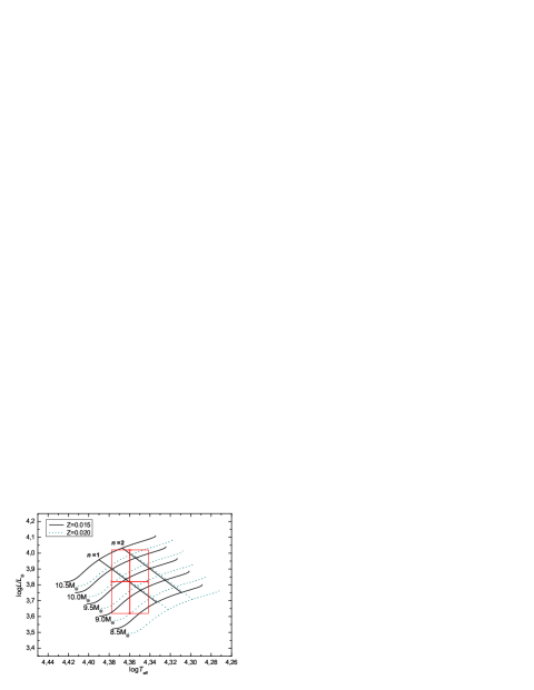
Figure 1: The observational error box of $\theta$ Ophiuchi in the HR diagram as determined from photometry by HSM05. The evolutionary tracks were computed with the OP-A04 opacities, assuming the rotational velocity of $V_{\rm rot}=30$ km/s, hydrogen abundance, $X=0.7$, two values of the metallicity parameter $Z$, and no overshooting from the convective core. We show also lines of constant period (0.1339 d) for the radial fundamental $(n=1)$ and the first overtone $(n=2)$ mode. These lines will be discussed later on.

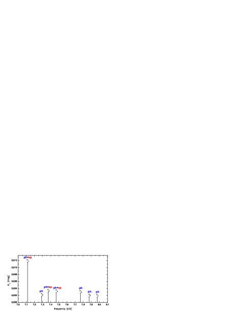
Figure 2: Oscillation spectrum of $\theta$ Ophiuchi. Seven frequencies were extracted from photometry (HSM05), marked as ${\bf ph}$, and three of them were found in spectroscopic variations (B05), marked as ${\bf sp}$.

The frequency analysis of time-series multicolour photometry of $\theta$ Oph, performed by HSM05, revealed seven pulsational frequencies in the range from 7.1160 to 7.9734 c/d. The dominant frequency ($\nu_{1}=7.1160$ c/d) corresponds to the earlier detected period (0.14 d) by McNamara (1957). Three of these seven frequncies were identified also in spectroscopy by B05. In Fig. 2, we show the oscillation spectrum of $\theta$ Oph. With ph we marked peaks detected in photometry and with ph+sp those three peaks detected both in photometry and spectroscopy.

3 Identification of pulsational modes of $\theta$ Oph

For the time being, mode identification in main sequence pulsators cannot be obtained from oscillation spectra themselves. Therefore, one has to rely on other observational quantities which bring information on the mode geometry. Such observables are, for example, amplitudes and phases of the multicolour photometric and radial velocity variations. Their theoretical values are computed under the assumptions of linear oscillation and plane-parallel, temporally static approximation for atmospheres. These assumptions are justified in the case of main sequence pulsators. If the effects of rotation on pulsation are ignored then the expression for the complex amplitude of the light variations in the passband $\lambda$ can be written in the form (see, e.g., Daszyńska-Daszkiewicz et al. 2002):

$${\cal A}_{\lambda}(i)=-1.086\varepsilon Y_{\ell}^{m}(i,0)b_{\ell}^{\lambda}(D_{1,\ell}^{\lambda}f+D_{2,\ell}+D_{3,\ell}^{\lambda})$$

where

$$D_{1,\ell}^{\lambda}=\frac{1}{4}\frac{\partial\log({\cal F}_{\lambda}|b_{\ell}^{\lambda}|)}{\partial\log T_{\rm{eff}}},$$

$$D_{2,\ell}=(2+\ell)(1-\ell),$$

$$D_{3,\ell}^{\lambda}=-\left(2+\frac{\omega^{2}R^{3}}{GM}\right)\frac{\partial\log({\cal F}_{\lambda}|b_{\ell}^{\lambda}|)}{\partial\log g_{\rm eff}}.$$

$\varepsilon$ is the mode intrinsic amplitude, $i$ is the inclination angle and $\ell,m$ are the spherical harmonic degree and the azimuthal order of the mode, respectively. Symbols $G,M,R,\omega$ have their usual meanings. The amplitudes and phases are given by $A_{\lambda}=|{\cal A}_{\lambda}|$ and $\varphi_{\lambda}=arg({\cal A}_{\lambda})$, respectively.

The term $D_{1,\ell}^{\lambda}$ describes temperature effects, $D_{2,\ell}$ - geometrical effects, and $D_{3,\ell}^{\lambda}$ - the influence of pressure changes. The terms $D_{1,\ell}^{\lambda}$ and $D_{3,\ell}^{\lambda}$ include the perturbation of the limb-darkening. $b_{\ell}^{\lambda}$ is the disc-averaging factor expressed as the integral of the limb-darkening weighted by the Legendre polynomial with the $\ell$ degree. Derivatives of the monochromatic flux, ${\cal F}_{\lambda}(T_{\rm eff},\log g)$, are calculated from static atmosphere models. In general, they depend also on the metallicity parameter [m/H] and microturbulence velocity $\xi_{t}$. Here, we use the Kurucz (2004) atmosphere models and Claret (2000) limb-darkening coefficients.

As was already mentioned in Introduction, the $f$ parameter describes the ratio of the bolometric flux perturbation to the radial displacement at the level of the photosphere:

$$\frac{\delta{\cal F}_{\rm bol}}{{\cal F}_{\rm bol}}={\rm Re}\{\varepsilon fY_{\ell}^{m}(\theta,\varphi){\rm e}^{-{\rm i}\omega t}\}.$$

The value of $f$ can be obtained from linear computations of stellar pulsation; because of nonadiabatic character of the pulsation, this quantity is complex. Here we use the pulsational code of W. Dziembowski.

If data on radial velocity variations are available, then the amplitude and phases of these variations can be included in a process of mode identification. The radial velocity is determined from observations as the first moment of well separated line profile, ${\cal M}_{1}^{\lambda}$. According to Dziembowski (1977), the expression for the complex amplitude of the radial velocity variations is the following

$${\cal A}_{\rm Vrad}={\cal M}_{1}^{\lambda}=\varepsilon Y_{\ell}^{m}(i,0){\rm i}\omega R\left(u_{\ell}^{\lambda}+\frac{GM}{\omega^{2}R^{3}}v_{\ell}^{\lambda}\right),$$

where $u_{\ell}^{\lambda}$, $v_{\ell}^{\lambda}$ are another disc-averaging factors introduced by Dziembowski (1977).

In principle, two approaches can be used in mode identification. The first approach makes use of amplitude ratios and phases differences and employs input from the pulsation theory, i.e., the $f$ parameter. In the linear and non-rotation approximation, the amplitude ratios and phases differences are independent of the intrinsic mode amplitude, $\varepsilon$, azimuthal order, $m$, and the inclination angle, $i$, because the factor $\varepsilon Y_{\ell}^{m}(i,0)$ cancels out.

The second method employs amplitudes and phases alone in order to determine from data the empirical values of $f$ and the intrinsic amplitude dependent on inclination, $\tilde{\varepsilon}=\varepsilon Y_{\ell}^{m}(i,0)$, together with the mode degree, $\ell$.

Both methods require input from models of stellar atmospheres.

3.1 Determination of the $\ell$ degree using photometry and theoretical values of $f$

Figure 3: Photometric diagnostic diagram for the $uy$ Strömgren passbands with positions of seven pulsational frequencies detected by Handler et al. 2005.

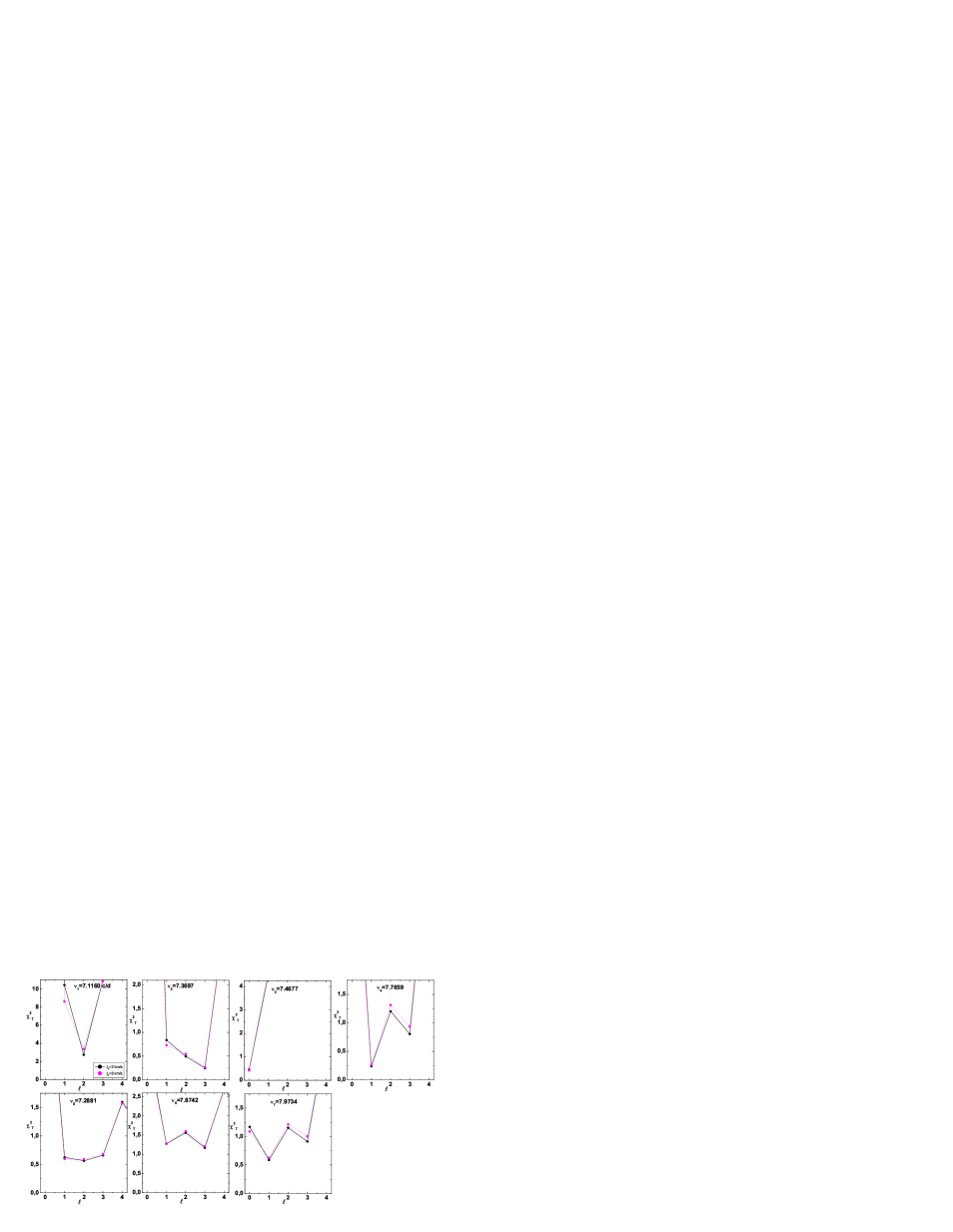
Figure 4: Identification of the $\ell$ degrees of the pulsational modes detected in the photometric variations using amplitude ratios and phase differences and theoretical $f$ parameter ($\chi^{2}_{T}~{}vs.~{}\ell$). These results correspond to the model with the following stellar parameters: $M=9.5M_{\odot},~{}\log T_{\rm eff}=4.363,~{}Z=0.015$, and computed with the OP-A4 opacity. The Kurucz atmosphere models were adopted. The effect of the microturbulence velocity, $\xi_{t}$, on the determination of $\ell$ is shown.

Observations of $\theta$ Oph in the $uvy$ Strömgren photometry were kindly provided by Gerald Handler. From these data we determined amplitudes and phases of the seven frequencies detected by HSM05 and, following HSM05, the amplitudes were corrected for the light contribution from the speckle companion: $A_{u}^{cor}=1.19A_{u},~{}A_{v}^{cor}=1.22A_{v},~{}A_{y}^{cor}=1.23A_{y}$. Although the phase differences between photometric passbands are small, they are not negligible, as shown in Fig. 3 for the $uy$ pair. Therefore, we included also these quantities to discriminate between various $\ell$ degrees. To this end we use, as usually, the following discriminant:

$$\chi^{2}_{T}=\frac{1}{2(N-1)}\sum_{i=1}^{N-1}\frac{(X_{i}^{o}-X_{i}^{t})^{2}}{\sigma_{i}^{2}},$$

where $X_{i}^{o},~{}X_{i}^{t}$ are observational and theoretical photometric observables, respectively, such as $A_{\lambda_{i}}/A_{\lambda_{1}}$ and $\varphi_{\lambda_{i}}-\varphi_{\lambda_{1}}$. N is the number of passbands and if we use only amplitude ratios we have to skip 2 in the denominator before the sum. The index ${\lambda_{1}}$ denotes the photometric passband to which the others, ${\lambda_{i}}$, are normalized and $\sigma_{i}$ are the observational errors of the $X_{i}^{o}$ quantities. Because we treat measurements in different passbands as independent variables, the formulae for errors ($\sigma_{i}$) are:

$$\sigma^{2}\left(\frac{A_{\lambda_{i}}}{A_{\lambda_{1}}}\right)=\left(\frac{A_{\lambda_{i}}}{A_{\lambda_{1}}}\right)^{2}\left[\frac{\sigma^{2}(A_{\lambda_{i}})}{A^{2}_{\lambda_{i}}}+\frac{\sigma^{2}(A_{\lambda_{1}})}{A^{2}_{\lambda_{1}}}\right],$$

and

$$\sigma^{2}(\varphi_{\lambda_{i}}-\varphi_{\lambda_{1}})=\sigma^{2}(\varphi_{\lambda_{i}})+\sigma^{2}(\varphi_{\lambda_{1}}).$$

We perform mode identification for the whole range of allowed stellar parameters and different values of metallicity.

In Fig. 4, we show results of our mode identification for the seven pulsational frequencies of $\theta$ Oph. This is an example for the model with parameters: $M=9.5M_{\odot},~{}\log T_{\rm eff}=4.363,~{}X=0.7,~{}Z=0.015$, computed with the OP-A04 opacities. The character of $\chi^{2}_{T}(\ell)$ for the other models is qualitatively the same. We consider stellar atmospheres with two values of the microturbulence velocity: $\xi_{t}=2$ and 8 km/s. In some cases a value of $\chi^{2}_{T}$ is less than 1 which comes from large observational errors.

Our identifications of the $\ell$ degrees agree with those obtained by HSM05 who used only photometric amplitudes. A discussion of the $\ell$ identification for each frequency will be given at the end of the next subsection.

3.2 Determination of the $\ell$ degree using empirical values of $f$

Three pulsational frequencies ($\nu_{1},~{}\nu_{2},~{}\nu_{3}$) were found in both photometric and spectroscopic observations of $\theta$ Oph. By combining these two types of data, we can identify the $\ell$ degree of these three frequencies and extract corresponding empirical values of the nonadiabatic $f$ parameter. In our analysis we use the radial velocity as determined by the first moment of the SiIII4553 spectral line. These data were kindly provided by Maryline Briquet. In our analysis we included only these spectra which coincide in time photometric observations.

Figure 5: Identification of the $\ell$ degrees of the pulsational modes detected in both photometry and in spectroscopy ($\chi^{2}_{E}~{}vs.~{}\ell$). Various lines correspond to uncertainties in the stellar parameters (see text for more explanation). The Kurucz atmosphere models with the microturbulence velocity of $\xi=2$ km/s were adopted.

The method of simultaneous determination of $\ell$ and $f$ has been described in details by DD03 and DD05, and we will not repeat this here. Each passband, $\lambda$, yields l.h.s. of Equations (1) whereas data on the radial velocity yield l.h.s. of Equation (4). This set of linear equations is solved for a specified $\ell$ in order to determine two complex unknown quantities: $\tilde{\varepsilon}$ and $\tilde{\varepsilon}f$. With three passbands and the radial velocity data we have a set of four complex equations. The idea is to derive the value of the nonadiabatic parameter $f$ and the intrinsic amplitude $\tilde{\varepsilon}$ from observations, which fit best the theoretical and observational amplitudes and phases for a given $\ell$ degree. The goodness of fit is calculated as

$$\chi^{2}_{E}=\frac{1}{2N-M}\sum_{i=1}^{N}\frac{|{\cal A}^{o}_{\lambda_{i}}-{\cal A}^{t}_{\lambda_{i}}|^{2}}{|\sigma_{\lambda_{i}}|^{2}},$$

where $N$ is the number of passbands plus one (to account for the fact that we use the radial velocity measurements) and $M$ is the number of parameters to be determined. Here $\lambda$ denotes either the photometric passband or radial velocity. ${\cal A}^{o}$ and ${\cal A}^{t}$ are complex observational and theoretical amplitudes, respectively, and $\sigma_{\lambda_{i}}$ are the observational errors. Because we treat amplitudes and phases as independent variables, the formula for the errors is

$$|\sigma_{\lambda}|^{2}=\sigma^{2}(A_{\lambda})+A_{\lambda}^{2}\sigma^{2}(\varphi_{\lambda}),$$

where $A_{\lambda}=|{\cal A}_{\lambda}|$ and $\varphi_{\lambda}=arg({\cal A}_{\lambda})$.

The results of mode identification by the above method for the first three frequencies of $\theta$ Oph are shown in Fig. 5. Various lines correspond to the uncertainties in the stellar parameters. We calculated $\chi^{2}_{E}$ for the models from the center and from the four edges of the error box in Fig. 1.

In Table 1 we give a summary of the $\ell$ identification from the two approaches. From both methods, the dominant frequency is undoubtedly a $\ell=2$ mode and the $\nu_{3}$ frequency is a radial mode. In the case of the $\nu_{2}$ frequency, we were able to exclude the $\ell=3$ degree from combined multicolour photometry and radial velocity data. For the remaining frequencies, we can rely only on mode identification from photometry alone. The three frequency peaks, $\nu_{4},~{}\nu_{6}$ and $\nu_{7}$, are equidistance and most probably form a close $\ell=1$ triplet. Other values of $\ell$ are also possible but because the disc averaging effects increase very rapidly with $\ell$, we regard these higher degrees as much less probable and assume, as HSM05, that this is the $\ell=1$ triplet. The $\ell=0$ identification for $\nu_{7}$ is of course excluded because $\nu_{7}$ is too close to $\nu_{3}$ which is the radial mode. The $\nu_{5}$ frequency can be identified either as $\ell$=1 or 2 or 3, with a lower probability for the $\ell=3$ identification. For the dominant mode, B05 identified also the azimuthal order, $m=-1$, on the basis of amplitudes and phases across the SiIII line profile.

Although there are some regularities in frequency spacing between $\nu_{1},~{}\nu_{5}$ and $\nu_{2}$, we are more cautious about believing that they are components of the same quintuplet. The regularities suggest that $\nu_{5}$ may be the $(\ell,m)=(2,+1)$ mode and $\nu_{2}$ - the $(\ell,m)=(2,+2)$ mode, as was assumed by Briquet et al. (2007) in their seismic analysis of $\theta$ Oph. However, from the amplitude and phase diagrams computed by B05 from variations of the SiIII line profile, the frequency $\nu_{3}=7.3697$ c/d looks rather like a $m=0$ mode, because the phase change is close to $\pi$ around the line center (see Fig. 3 of B05).

Thus, our complex seismic analysis we will be based on frequencies $\nu_{3}$ and $\nu_{6}$ which are well identified centroid modes with $\ell=0$ and $\ell=1$, respectively, and we postpone studies of rotational effect until more than one multiplet will be well identified.

Table 1: Summary of mode identification using two methods for frequency peaks detected in $\theta$ Ophiuchi.

Frequency [c/d]	photometry	photometry+$V_{\rm rad}$
	theoretical $f$ parameter	empirical $f$ parameter
$\nu_{1}$= 7.11600	$\mathbf{\ell=2}$	$\mathbf{\ell=2}$
$\nu_{2}$= 7.3697	$\mathbf{\ell=3,2,1}$	$\mathbf{\ell=1,2}$
$\nu_{3}$= 7.4677	$\mathbf{\ell=0}$	$\mathbf{\ell=0}$
$\nu_{4}$= 7.7659	$\mathbf{\ell=1,3}$	–
$\nu_{5}$= 7.2881	$\mathbf{\ell=1,2,3}$	–
$\nu_{6}$= 7.8742	$\mathbf{\ell=1,3,2}$	–
$\nu_{7}$= 7.9734	$\mathbf{\ell=1,3,2,0}$	–

3.3 Determination of the radial orders

In Fig. 1 we have plotted lines of a constant period (0.1339 d) for fundamental ($n=1$) and first overtone ($n=2$) radial mode. These line correspond to $\nu_{3}=7.4677$ c/d. As we can see, within the allowed space of stellar parameters there are two possible identifications for the radial order: $n=1$ or $n=2$. To discriminate between these two identifications, we shall use results from the method of DD03 (Section 3.2).

Firstly, we can calculate values of $\chi^{2}_{E}$ as a function of effective temperature for the case of $n=1$ and $n=2$. This is shown in Fig. 6. The vertical lines mark the allowed range of $\log T_{\rm eff}$. Although the fundamental mode takes lower values of $\chi^{2}_{E}$, we cannot exclude the first overtone from this graph because both lines reach acceptable values of $\chi^{2}_{E}$.

Another way to discriminate between the two radial orders for the $\ell=0$ mode is to compare theoretical and empirical values of the nonadiabatic $f$ parameter (see DD05). The photometric and spectroscopic data for $\theta$ Oph allowed to determine the values of $f$ for the $\nu_{3}$ mode with sufficient accuracy to use them to this aim. In Fig. 7 we show such comparison. Only models with stellar parameters within the error box of Fig. 1 were considered. As we can see, the $n$ identification is clear and $\nu_{3}$ is the radial fundamental mode. In addition, lines of constant values of the instability parameter, $\eta=0$, are shown. Only models to the right of this line have unstable radial modes. In Fig. 7, we show also the sensitivity of the theoretical $f$ parameter to metallicity prameter $Z$. A comparison of theoretical and empirical values of $f$ gives also additional support to the result that metallicity of $\theta$ Oph is lower than $Z=0.015$.

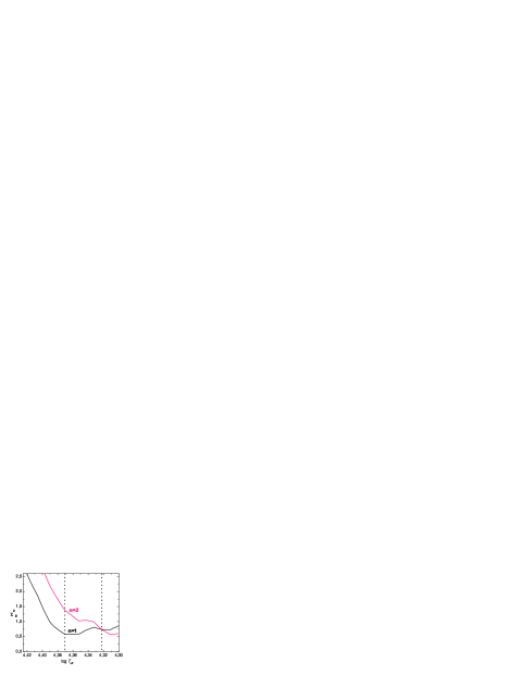
Figure 6: The $\chi^{2}_{E}$ as a function of the effective temperature for the frequency $\nu_{3}$ identified as the l=0 mode. Two possible values of the radial order, $n$, were considered. Vertical dotted lines indicate the allowed range of $\log T_{\rm eff}$.

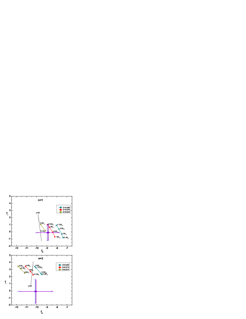
Figure 7: Comparison of empirical and theoretical values of the $f$ parameter for the radial mode $\nu_{3}$. The upper panel refers to the fundamental mode hypothesis and the lower one, to the first overtone mode hypothesis. Theoretical values of $f$ were calculated with the OP-A04 opacities, metallicity $Z=0.020$, 0.015 and 0.012, and assuming stellar parameters within the error box. Lines of constant values of the instability parameter, $\eta$, are labeled as $\eta=0$.

After fixing the $n$ order of the $\nu_{3}$ radial mode as $p_{1}$, we can try to associate the radial orders also for other frequencies. A survey of pulsational models showed that the $\ell=1$ triplet can be identified as $p_{1}$, whereas the dominant $(\ell,m)=(2,-1)$ mode, as a component of the $g_{1}$ quintuplet.

4 Constraints on intrinsic mode amplitudes

Having determined the value of $\tilde{\varepsilon}=\varepsilon Y_{\ell}^{m}(i,0)$ from the method of DD03 in Section 3.2, we can get a lower limit for the value of the intrinsic mode amplitude, $\varepsilon$, and, in the case of a radial mode, its exact value. The available observations of $\theta$ Oph allow to determine the values of $\tilde{\varepsilon}$ for $\nu_{1}$ and $\nu_{3}$ with a sufficient accuracy.

The dominant mode, $\nu_{1}$, is unequivocally the $\ell=2$ mode. Moreover, from spectroscopic time series analysis B05 identified its azimuthal order as $m=-1$. With these angular numbers, we can calculate the intrinsic amplitude of the dominant mode as a function of the inclination angle. The result is shown in Fig. 8. As one can see, inclination angles close to $85-90^{\circ}$ are excluded because of the node line of the $(\ell,m)=(2,-1)$ mode. The minimum value of the intrinsic amplitude of the dominant mode is equal to 0.0098 at i=45^∘, i.e. 0.98% of the stellar radius. In the case of the $\nu_{3}$ frequency, which correspond to the radial mode, we estimated the exact value of $\varepsilon$ as 0.0014, i.e. 0.14% of the stellar radius. These estimates mean that the intrinsic amplitude of the dominant $(\ell,m)=(2,-1)$ mode is at least 7 times larger than that of the radial mode. Here the open problem of mode selection emerges and such determinations can bring us closer to a solution.

Figure 8: The intrinsic amplitude of the dominant mode, $\nu_{1}$, $(\ell,m)=(2,-1)$, as a function of the inclination angle. The minimum value of $\varepsilon(\nu_{1})$ is equal to about 0.01. The value of $\varepsilon$ for the radial mode, $\nu_{3}$, is plotted as the dotted line.

5 Complex asteroseismic modelling

We shall perform our seismic modelling in two steps. Firstly, we find a family of models which fit the two centroid frequencies of $\theta$ Ophuichi, i.e., $\nu_{3}$, which was identified as the $\ell=0,p_{1}$ mode, and $\nu_{6}$, which is the centroid of the $\ell=1,p_{1}$ triplet. In the next step, from this set of models we will select only those which reproduce, within the observational errors, the empirical values of $f$ of the radial fundamental mode.

5.1 Fitting frequencies of the $\ell=0$ mode and the $\ell=1$ centroid mode.

To construct our seismic models, we use two frequencies: $\nu_{3}=7,4677$ (the $\ell=0$ mode) and $\nu_{6}=7.8742$ c/d (the $\ell=1$ centroid mode), because the $\nu_{1}$ frequency is a non-axisymmetric $\ell=2$ mode with $m=-1$, while frequencies $\nu_{2}$ and $\nu_{5}$ do not have unambiguous identification. We searched for models fitting these two frequencies by changing various parameters: the mass, $M$, the effective temperature, $T_{\rm eff}$, the chemical abundance, ($X,Z$), and the core overshooting parameter, $\alpha_{\rm ov}$. The effect of overshooting was computed according to the new formulation of Dziembowski & Pamyatnykh (2008). This new treatment takes into account not only the distance of the overshooting but also partial mixing in the overshoot layer. In our seismic modelling, we relied on the latest determination of the solar element mixture by A04 and used both the OP tables (Seaton 2005) and OPAL tables (Iglesias & Rogers 1996). The rotational splitting for the $\ell=1$ triplet is about 0.1 c/d, giving the rotational velocity of $V_{\rm rot}=30$ km/s for the stellar radius of about $R=6R_{\odot}$; this is consistent with the $V_{\rm rot}\sin i$ value derived by Abt, Levato & Grosso (2002) mentioned in Section 2. We assumed this value of $V_{\rm rot}$ in all computations.

In Fig.9 we show the results of our seismic modelling for the OP data on the $\alpha_{\rm ov}~{}vs.~{}Z$ plane. The instability borders are labeled with $\eta=0$ and shown as the thick solid and thick dotted lines for the $\ell=0$ and $\ell=1$ modes, respectively. Only models above those lines are unstable and reproduce the observed frequencies $\nu_{3}$ and $\nu_{6}$. Moreover, we depicted also the lines of constant mass and effective temperature. We show results for two values of hydrogen abundance: $X=0.7$ (the left panel) and $X=0.75$ (the right panel).

From such data, one can easily find the relation for a family of seismic models for a fixed value of $X$ in the form:

$$\alpha_{\rm ov}=a\cdot M+b\cdot\log T_{\rm eff}+c\cdot Z+d.$$

As we can see, models with lower $Z$ require more core overshooting. This is because for a higher value of $Z$ the convective core is larger, implying a lower value of the overshooting distance. The same result was obtained by Briquet et al. (2007) for $\theta$ Oph and by Dziembowski & Pamyatnykh (2008) in their studies of hybrid pulsators, $\nu$ Eri and 12 Lac. A similar dependence was also obtained for lower mass stars (M.-J. Goupil, private communication). On the other hand, at a given metallicity, for a higher value of $X$ we need higher value of $\alpha_{\rm ov}$ to get pulsational instability.

All these seismic models of $\theta$ Oph prefers lower effective temperatures and lower masses. The lower effective temperature limit is $\log T_{\rm eff}\approx 4.34$, thus most of these seismic models are outside the error box. We would like to mention that a lower value of effective temperature was determined from the IUE spectra by Niemczura& Daszyńska (2005) who derived $\log T_{\rm eff}=4.347\pm 0.016$. The ultraviolet spectra of the $\theta$ Oph system are dominated by the main component, i.e. the early B-type star, which emits most energy in UV and dominates this part of spectrum. Therefore, this lower value of $\log T_{\rm eff}$ can be more reliable and it is also more consistent with seismic models. The higher value of $X$ require even lower values of $\log T_{\rm eff}$. The effect of the opacity tables will be discussed in the next section.

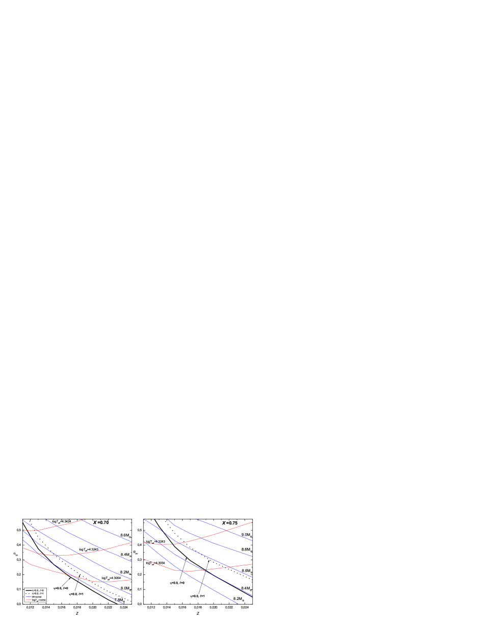
Figure 9: The overshooting parameter as a function of metallicity for the seismic models of $\theta$ Oph found from the fitting of the $\nu_{3}$ frequency (the $\ell=0,p_{1}$ mode) and the $\nu_{6}$ frequency (the centroid of the $\ell=1,p_{1}$ triplet). Results for two values of the hydrogen abundance, $X$, are shown: 0.70 (the left panel) and 0.75 (the right panel).

5.2 Fitting the $f$ parameter of the $\ell=0,p_{1}$ mode

Determination of empirical values of $f$ puts additional and unique constraints on seismic models. In that way, we are going one step further by a requirement of fitting simultaneously pulsational frequencies and the corresponding values of $f$. The sensitivity of the theoretical $f$ parameter to metallicity is very strong and was already shown in Fig. 7. How this quantity depends on the hydrogen abundance, overshooting distance and adopted opacity tables is demonstrated in Fig. 10. As we can see, the strongest effect comes from opacity data. The amount of hydrogen and the overshooting distance have a minor effect on the value of $f$.

From a set of seismic models found in Section 5.1, we singled out only those which have the $f$ parameter for the radial mode consistent with the observed values within the errors. Having also another source of opacity data, we studied the effect of this input on the seismic models. In Fig. 11 we plotted similar diagrams as in Fig. 9, but at a fixed hydrogen abundance ($X=0.7$) and considering both the OP tables (the left panel) and the OPAL tables (the right panel). Moreover, we superimposed areas resulting from fitting empirical values of $f$ for the radial mode. As we can see, only models calculated with the OPAL tables can account for the empirical $f$ parameters with a reasonable value of the overshooting distance. An interesting fact is that with both opacity tables it was possible to reproduce the real parts of $f$ for lower values of $\alpha_{\rm ov}$, whereas only the OPAL data gave consistency also in the imaginary parts of $f$. This is a very important and revealing result. It shows how complex asteroseismic studies can test data on microscopic physics. Another support for the OPAL data is that with these opacities we get also a better agreement between stellar parameters of seismic models and those derived from photometric or spectroscopic observations.

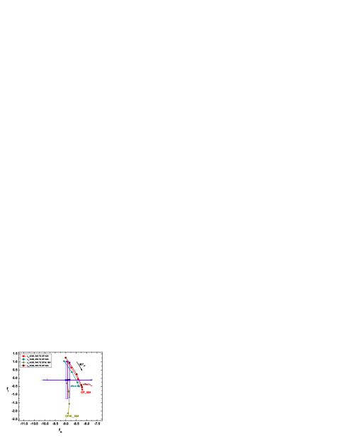
Figure 10: A comparison of empirical and theoretical values of $f$ for the radial mode of $\theta$ Oph. Theoretical $f$ parameters were computed for different values of the hydrogen abundance, $X$, the overshooting parameter, $\alpha_{\rm ov}$, and for two sources of opacity data. The A04 solar chemical mixture was adopted and metallicity fixed at Z=0.015.

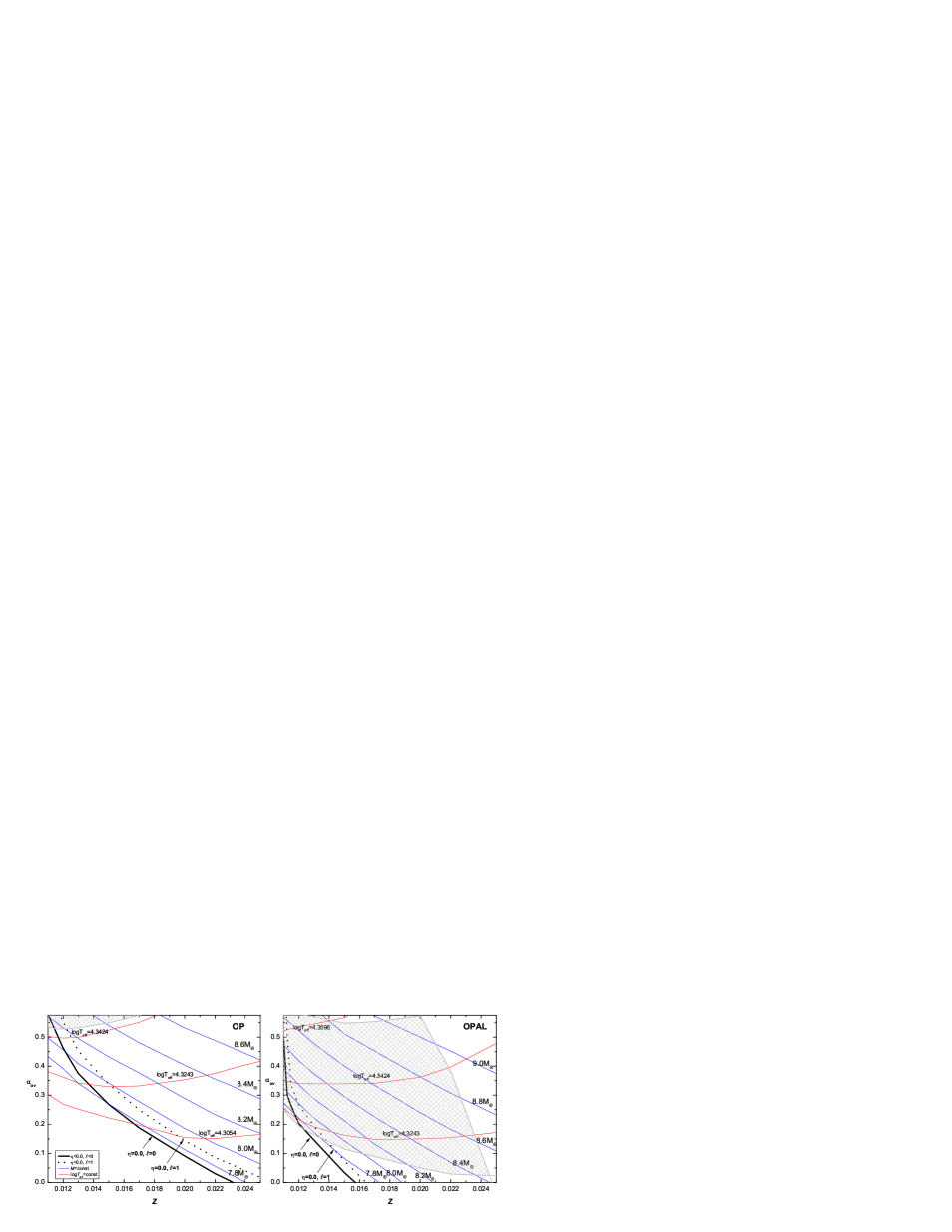
Figure 11: The overshooting parameter as a function of metallicity for the seismic models of $\theta$ Oph found from the fitting of the $\nu_{3}$ frequency (the $\ell=0,p_{1}$ mode) and the $\nu_{6}$ frequency (the centroid of the $\ell=1,p_{1}$ mode). Results were obtained with the OP (the left panel) and the OPAL table (the right panel). The hatched areas mark the models which fit the $f$ parameter for the radial fundamental mode.

6 Summary

Our analysis showed a great potential of probing parameters of stellar models and microphysics by means of the nonadiabatic parameter $f$. Incorporating this quantity in seismic modelling provides much stronger constraints and a new kind of information. The adequate seismic model should account not only for oscillation frequencies but also for the empirical values of $f$, visibility and instability conditions. This kind of seismic modelling we called complex asteroseismology. The aim of the complex asteroseismic analysis is to find stellar models which fit both oscillation frequencies and corresponding $f$ parameters. The value of $f$ is determined in subphotospheric layers which only weakly affect the pulsational frequencies. Therefore, these two asteroseismic tools ($\nu,f$) are complementary to each other and treating them simultaneously can improve seismic modelling of any kind of pulsating stars. As was already discussed by DD05, for B-type pulsators, the $f$ seismic tool probes in particular stellar metallicity and opacities. In this paper, we have demonstrated that even with data on only two well identified centroid modes and the empirical $f$ parameter for the radial mode we can derive very strong constraints on stellar parameters, core overshooting and, in particular, on opacities.

Our analysis of $\theta$ Ophiuchi showed that only with the OPAL table it was possible to reproduce simultaneously the two pulsational frequencies and the empirical value of $f$ corresponding to the radial mode. Seismic models obtained with the OP data require enormous amounts of core overshooting, at least $\alpha_{\rm ov}=0.55$, which we consider not physical for a mass and rotational velocity appropriate for $\theta$ Oph. Computations with the OPAL tables allowed to achieve agreement between observed and theoretical values of $f$ for a wide space of parameters, $(M,T_{\rm eff},\alpha_{\rm ov},Z)$, fixed by the mode frequency fitting. Such complex asteroseismic studies provide a critical and unique test for stellar opacities and the atomic physics.

Another important results of this paper are valuable constraints on the intrinsic amplitude for the dominant $(\ell=2,m=-1)$ mode and for the $\ell=0$ mode. We have found out that the dominant mode of $\theta$ Oph has to be excited with the intrinsic amplitude at least seven times larger than the radial mode. Although, in the framework of linear theory, we cannot compare these values with theoretical predictions, such estimates can give us some guidelines to the mode selection mechanism in the $\beta$ Cephei pulsators.

References

- (1) Abt H. A., Levato H., Grosso M., 2002, ApJ, 573, 359
- (2) Aerts, C., Toul, A., Daszyńska, J., et al., 2003, Science, 300, 1926
- (3) Aerts, C., de Cat, P., Handler, G., et al., 2004, MNRAS, 347, 463
- (4) Asplund M., Grevesse N., Sauval A. J., Allende Pieto C., Kisleman D., 2004, A&A, 417, 751 (A04)
- (5) Asplund M., Grevesse N., Sauval A. J., 2005, in Barnes T. G. III, Bash F. N., eds, ASP Conf. Ser. Vol. 336, Cosmic Abundances as Records of Stellar Evolution and Nucleosynthesis. Astron. Soc. Pac., San Francisco, p. 25
- (6) Ausseloos, M., Scuflaire, R., Thoul, A., Aerts, C., 2004, MNRAS, 355, 352
- (7) Briquet, M., Lefever, K., Uytterhoeven, K., Aerts, C. , 2005, MNRAS, 362, 619 (B05)
- (8) Briquet, M., Morel, T., Thoul, A., et al. 2007, MNRAS, 381, 1482
- (9) Claret, A., 2000, A&A, 363, 1081
- (10) Daszyńska, J., 2001, PhD Thesis, Wrocław University
- (11) Daszyńska-Daszkiewicz J., Dziembowski W. A., Pamyatnykh A. A., Goupil M.-J., 2002, A&A, 392, 151
- (12) Daszyńska-Daszkiewicz J., Dziembowski W. A., Pamyatnykh A. A., 2003, A&A, 407, 999 (DD03)
- (13) Daszyńska-Daszkiewicz J., Dziembowski W. A., Pamyatnykh A. A., 2005a, A&A, 441, 641 (DD05)
- (14) Daszyńska-Daszkiewicz, J., Dziembowski, W. A., Pamyatnykh, A. A., Breger, M., Zima, W., Houdek, G., 2005b, A&A, 438, 653
- (15) Dziembowski, W. A., 1977, AcA, 27, 203
- (16) Dziembowski, W. A., Jerzykiewicz, M., 1996, A&A, 306, 436
- (17) Dziembowski, W. A., Jerzykiewicz, M., 1999, A&A, 341, 480
- (18) Dziembowski, W. A., Pamyatnykh, A. A., 2008, MNRAS, 385, 2061
- (19) Handler, G., Shobbrook, R. R., Jerzykiewicz, M. et al., 2004, MNRAS 347, 454
- (20) Handler, G., Shobbrook, R. R., Mokgwetsi, T., 2005, MNRAS 362, 612 (HSM05)
- (21) Handler, G., Jerzykiewicz, M., Rodriguez, E., et al., 2006, MNRAS 365, 327
- (22) Handler, G., Matthews, J. M., Eaton, J. A., et al., 2009, ApJ 698, L56
- (23) Henroteau, F., 1922, Publ. Dom. Obs. Ottawa, 8, 1
- (24) Iglesias, C. A., Rogers, F. J., 1996, ApJ 464, 943
- (25) Jerzykiewicz, M., Handler, G., Shobbrook, R. R. et al., 2005, MNRAS 360, 619
- (26) Kurucz, R. L., 2004, http://kurucz.harvard.edu
- (27) McAlister H., Mason B. D., Hartkopf W. I., Shara M. M., 1993, AJ, 106, 1639
- (28) McNamara, D. H., 1957, PASP, 69, 574
- (29) Niemczura, e., Daszyńska-Daszkiewicz J., 2005, A&A, 433, 659
- (30) Pamyatnykh, A. A., Handler, G., Dziembowski, W. A., 2004, MNRAS 350, 1022
- (31) Seaton, M. J., 2005, MNRAS, 362, L1
- (32) Stankov, A., Handler G., 2005, ApJS, 158, 193