An investigation of lucky imaging techniques

Abstract

We present an empirical analysis of the effectiveness of frame selection (also known as Lucky Imaging) techniques for high resolution imaging. A high-speed image recording system has been used to observe a number of bright stars. The observations were made over a wide range of values of $D/r_{0}$ and exposure time. The improvement in Strehl ratio of the stellar images due to aligning frames and selecting the best frames was evaluated as a function of these parameters. We find that improvement in Strehl ratio by factors of 4 to 6 can be achieved over a range of D/r₀ from 3 to 12, with a slight peak at $D/r_{0}\sim 7$. The best Strehl improvement is achieved with exposure times of 10 ms or less but significant improvement is still obtained at exposure times as long as 640 ms. Our results are consistent with previous investigations but cover a much wider range of parameter space. We show that Strehl ratios of $>$0.7 can be achieved in appropiate conditions whereas previous studies have generally shown maximum Strehl ratios of $\sim$0.3. The results are in reasonable agreement with the simulations of Baldwin, Warner & Mackay (2008).

1 Introduction

The frame selection technique for high resolution imaging involves the recording of a time series of short exposure images and the selection of the sharpest images out of the series for alignment and combining into a final image. Fried (1978) determined that the probability of obtaining a lucky sharp image (defined as one with wavefront variance less than $1rad^{2}$) with a telescope of aperture $D$ in seeing described by a Fried parameter $r_{0}$ (Fried, 1967) is given by:

$$P=5.6exp[-0.1557(D/r_{0})^{2}]$$ (1)

This suggests that there will be more good quality images available at low $D/r_{0}$. The probability of such an image is 1 in 9 for $D/r_{0}=5$ or 1 in 50 for $D/r_{0}=6$. For higher $D/r_{0}$ the probability of a sharp image rapidly decreases, being 1 in 3800 for $D/r_{0}=8$. Since the image quality gain will increase with $D/r_{0}$ this suggests the frame selection techique will work best for $D/r_{0}\sim 6-7$, this being the largest $D/r_{0}$ at which there is a good chance of finding several high quality images in a typical image sequence of a few thousand frames.

There have been a number of practical demonstrations of this technique variously described as frame selection (Roggemann & Welsh, 1996), lucky imaging (Law et al., 2006), or selective image reconstruction (Dantowitz, Teare & Kozubal, 2000). Baldwin et al. (2001) demonstrated the ability to obtain diffraction limited star images at 800nm wavelength with a 2.5m telescope.

The technique has been used to image the hemisphere of Mercury that was missed by Mariner 10 (Dantowitz, Teare & Kozubal, 2000; Cecil & Rashkeev, 2007; Ksanfomality & Sprague, 2007) and is now widely used by amateur astronomers for planetary imaging.

Interest in the technique is rapidly increasing, in part due to the availability of electron multiplying CCD (EMCCD) technology, which allows rapid readout of CCDs with negligible read noise (Mackay et al., 2001), as well as computers with fast processors and large storage capacity. A number of such systems have recently been demonstrated, for example LuckyCam (Law et al., 2006), AstraLux (Hormuth et al., 2008) and FastCam (Oscoz et al., 2008).

However, previous studies have generally been aimed at obtaining the best possible image resolution and have therefore explored a restricted range of parameters. In this paper we present observations that explore a wide range of parameter space. We have explored empirically the effects of telescope aperture $D$, wavelength $\lambda$, frame exposure time $t$ and frame selection rate $FSR$ on the resulting image quality. Unlike most previous studies which have aimed at exploiting excellent seeing conditions, our observations were obtained in a range of seeing conditions from good to poor. The results provide information that can help to optimize the design of future instruments.

2 Observations

The observations were obtained using MUSIC Mk I (Macquarie University Selective Imaging Camera). The study was carried out as a preliminary stage in the design of a more advanced lucky imaging system that will use an electron multiplying CCD camera. The imager used for MUSIC was a Watec 100N monochrome video camera. This camera was chosen because it had adjustable exposure times and adequate sensitivity to observe bright stars. The observations used standard BVRI filters. The camera was placed either directly at the telescope focus, or when necessary used with a 2.5 times focal extender. In all cases the image scale was chosen to ensure that the pixels provided good sampling of diffraction limited star images.

The camera produces video output with an effective pixel size of 8.6 by 8.3 $\mu$m and a format of 768 by 576 pixels. The camera generates video data with interlaced scanning (i.e. each frame consists of consecutive scans of odd rows and even rows stitched together). The video data was recorded using a Data Translation DT3155 PCI frame grabber mounted in a PC system using a 3GHz Pentium 4 processor. The PC was configured with 1 TB of disk space (two 400 Gb and one 200 GB drives) to record the large data files. The operating system was Fedora Core Linux. A data acquisition software system was developed that enabled data from the video camera to be recorded continuously as three dimensional FITS files, while being displayed in real time. The software made use of C++ classes developed at the Anglo-Australian Observatory for the IRIS2 project and AAO2 detector controllers (Shortridge et al., 2004). The image display was based on the ESO Real Time Display (RTD) system (Herlin, Brighton & Biereichel, 1996). The system was capable of recording full frame video data to disk for extended periods. Typical observations consisted of sequences of 3000 to 10000 video frames.

MUSIC was used on three telescopes. The observing dates, locations and instruments used are summarised in table 1. The bulk of the observations were obtained on the 1m ANU telescope at Siding Spring Observatory. A small number of observations were obtained on the 3.9m Anglo-Australian Telescope (AAT, also at Siding Spring) and on the 0.4m telescope of the Macquarie University Observatory in Sydney.

One aim of the observations was to explore the effects of changes in $D/r_{0}$, which may be regarded as the seeeing-normalised aperture. While natural variation in seeing provides changes in $r_{0}$, we also varied $D$ by placing masks of different size over the telescope aperture. With the 1m telescope we used mask sizes of 75cm, 30cm, 20cm and 10cm, with the smaller masks being placed off-centre to avoid the central obstruction of the secondary mirror. With the AAT off-centre masks corresponding to apertures from 40cm to 1.0m were used located at the top of the “chimney” above the primary mirror central hole. A 2.5m aperture was also achieved by closing down the primary mirror covers.

The frame exposure times used ranged from $1-20ms$ on the camera. Additional runs with exposure times from $40-640ms$ were simulated by combining groups of consecutive frames from the $20ms$ runs.

Observations were made of a number of bright stars, as well as of some clusters and binaries of various angular separations to test the effects of selective imaging on image sharpness across the field. In each case observations were recorded with a range of different exposure times, and through different filters.

Table 1: Summary of MUSIC Observing Runs

Date	Location	Instrument
2005 Mar 8	Macquarie University,	Meade 40cm
	Sydney NSW
2005 Mar 11-23	Siding Spring, NSW	ANU 1m
2005 Jun 25	Siding Spring, NSW	AAT 3.9m
2005 Nov 9-14	Siding Spring, NSW	ANU 1m

Frames in each FITS cube were calibrated by bias subtraction and flat fielding (using exposures of the daylight sky). With our camera, the odd and even rows in each interlaced scan represent two consecitive exposures. Therefore each frame was de-interlaced by separating the odd and even rows into separate frames and filling the gaps by interpolation. This produced calibrated FITS cubes with twice as many frames as the raw ones. Also, in order to maintain precision the new data cubes were saved in floating point format.

We used a simple peak pixel algorithm (Aspin et al., 1997) for aligning and selecting frames. This relies on the fact that noise in the image is minimal, which is generally the case for the bright stars oberved. Different techniques would be needed for fainter guide stars. We therefore use the value of the highest pixel in each frame as a measure of image quality, since sharper stellar images will have more flux in the central peak. Post-processing was done by scanning each cube to find the brightest pixel in each frame, and then the frames were ranked in order of peak pixel value. The desired fraction of best frames, defined by the frame selection rate ($FSR$), were aligned so that the position of the peak pixel in each frame coincided with that in the best frame and then average-combined (“shift-and-added”). Frame selection rates of 100%, 10% and 1% were used. These were compared with simulated long exposures made by combining all frames with no alignment (“stacking”).

We used the Strehl ratio as a measure of the quality of the resulting star images. Another possible measure is the full width at half maximum (FWHM) of the image. However, this is not, in practice, a good measure of image quality. Images resulting from frame selection generally have a core-halo structure; i.e. a diffraction limited core surrounded by an extended halo the size of the original seeing disk. The core can give rise to a small FWHM even though most of the energy is in the halo. Strehl ratio is a much more demanding measure of image quality, since a high Strehl ratio can only be achieved if most of the energy is in the diffraction limited core. We measured the Strehl ratios using the “strehl” command of the ESO Eclipse software package  (Devillard, 2001). This works by comparing the observed images with a simulated diffraction-limited point spread function, which takes into account, where appropriate, the central obstruction of the aperture in a Cassegrain telescope.

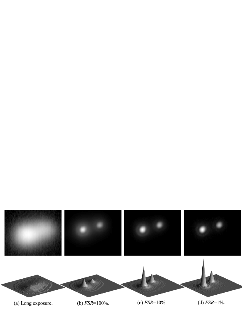
Figure 1: Images of binary star $\tau$Ophiuchii (1.7” separation) produced by selective imaging. Images in the top row are brightness-normalised and logarithmic pixel scale to highlight the faint halo. The 3-dimensional plots in the bottom row are linear scale, and show increasing peaks with decreasing $FSR$. Images were taken on the AAT, $D=40cm$ aperture mask, $t=120ms$, $\lambda=0.7\mu$m filter.

3 Discussion

3.1 Frame Selection Rate $FSR$

The stellar images produced by frame selection shown in figure 1 are among our best results. Note that the images in the top row are displayed brightness-normalised and logarithmic pixel scale to highlight faint features. In figure 1(a) the frames were stacked, simulating a long exposure image. The next image has all frames shift-and-added ($FSR=100\%$), which is equivalent to tilt correction. The binary is well resolved with a separation of 1.7 arcseconds that matches published values. Both stars have a clear central peak with a significant halo. The third and fourth images have the best 10% and 1% of frames aligned and combined. This removed those frames with the greatest speckling caused by high order wavefront distortions. The result is greater flux in the central peak and a fainter halo. In the 1% $FSR$ image there is a dark ring at a radius of 8 pixels from each peak, matching the Rayleigh criterion for a diffraction limited image. The 3-dimensional plots show the diminishing halo and increasing brightness of the peaks with decreasing $FSR$, which is not shown by the brightness-normalised images. The Strehl ratios for both peaks in each frame-selected image listed in table 2 verify the quality improvement, with the $FSR=1\%$ image having a Strehl raio of almost 0.8.

The Strehl ratios listed in table 2 illustrate an important effect of shift-and-add processing. In the long exposure image the two peaks are unresolved so no Strehl ratio measurement is possible. In each of the frame selected images the Strehl ratio of the secondary peak is higher than that in the long exposure, but in all cases is less than the corresponding primary peak. This is because even frames with high overall sharpness may still contain more than one isoplanatic patch. When frames are co-aligned on the brightest pixel the Strehl ratio of the primary peak is artificially enhanced. Other peaks may have a different tilt and speckle pattern. Shift-and-adding may still improve the sharpness of these features, but to a lesser extent than the primary peak, as seen in figure 1 and table 2. Our data shows a general trend to diminishing Strehl ratio and less Strehl improvement with increasing angular distance from the alignment location. This trend seems to be largely independent of $FSR$ and $D/r_{0}$. This is in qualitative agreement with the simulations by Baldwin, Warner & Mackay (2008), though a direct quantitative comparison is not possible. However in all of our observations the secondary peaks showed improvement with frame selection, even over angular separations as large as 100 arcseconds.

Table 2: Strehl ratios of peaks in images in figure 1

	Frame Selection Rate
Peak	100%	10%	1%
Primary	0.517	0.654	0.799
Secondary	0.362	0.547	0.674
Secondary/Primary	69.9%	83.7%	84.4%

3.2 Seeing-normalised aperture $D/r_{0}$

We determined $r_{0}$ from the FWHM of the long exposure image using the standard relationship $FWHM=0.98\lambda/r_{0}$. Over all of our observations $r_{0}$ ranged from 1 to 12cm, and $D/r_{0}$ from 2.8 to 30.3. Figure 2 plots bin-averaged Strehl ratios of stellar image versus $D/r_{0}$ between 3.0 and 12.0. For $D/r_{0}>12.0$ the trends continue more or less flat. For $D/r_{0}<12.0$ the obvious trend is for higher Strehl ratios in better seeing (large $r_{0}$) and/or with smaller aperture (small $D$). With low $D/r_{0}$, not only are there more good frames to choose from (one could use a quality threshold instead of frame selection rate) but the average frame quality is better, as indicated by higher Strehl ratios of the long exposure images in this region. This makes frame selection most suitable for use with small to medium sized telescopes at visible wavelengths. This does, however, limit the magnitudes of usable target objects or guide stars.

Figure 3 shows the quality improvement versus $D/r_{0}$. The improvement factor was measured by the gain in the Strehl ratio; that is, the Strehl ratio of a frame selected image divided by that of the long exposure image derived from the same image cube. Figure 3 compares the improvement made by pure shift-and-add ($100\%FSR$) with that from $1\%FSR$. The $1\%FSR$ points are consistently higher than those for $100\%FSR$, confirming the advantage of being more selective. The $1\%FSR$ images show an improvement factor greater than 5 for $D/r_{0}$ between 4.5 and 7.8, with a small peak at $D/r_{0}\sim 7$. This represents the best compromise between the diffraction-limited resolution, which improves with increasing $D$, and seeing-limited resolution that improves with increasing $r_{0}$. Nevertheless the peak is not very pronounced, and substantial Strehl ratio improvement is obtained at all values of $D/r_{0}$.

Data from our individual observations is displayed in figure 4 compared with results from other experiments. In this plot our data are limited to $t\leq 4ms$ and $D/r_{0}\leq 12$, $1\%$ and $100\%FSR$. The crosses are previous lucky imaging results (Baldwin et al., 2001; Law et al., 2006; Hormuth et al., 2008) and match our data well, even though our data was generally obtained in poorer seeing but with smaller apertures. However, these previous studies generally targeted the optimum case of $D/r_{0}\sim 7$, and acheved maximum Strehl ratios of $\sim 0.3$. Our data show that smaller $D/r_{0}$ values can be used to achieve higher strehl ratios of $>0.6$ and in a few cases as high as 0.8. The high Strehl ratios for the images in figure 1 were achieved with $D/r_{0}=3.84$.

The line in figure 4 is the simulation from Baldwin et al. (2008). It can be seen that the simulation line lies at the upper boundary of the scatter of points. Typically both our observations and previous results lie below the simulation. This is probably due to aberrations in the optics of the telescopes employed. The simulated case assumes a diffraction limited telescope. In this case frame selection will select those images in which the wavefront distortion due to turbulence is minimal. When using a real telescope with aberrations it is necessary instead to select those frames in which the turbulence induced wavefront distortions cancel out those due to telescope aberrations. The probability of a ”lucky image” in this case is lower than that for a perfect difraction limited telescope (Beckers & Rimmele, 1996) and hence the image quality gain from frame selection is reduced.

3.3 Colour band $\lambda$

Because $r_{0}\propto\lambda^{6/5}$ (Fried, 1966) it was expected that the better Strehl ratios would be achieved at longer wavelengths due to the larger $r_{0}$ patch. Table 3 shows the ranges of $r_{0}$, $D/r_{0}$ and long exposure (stacked) Strehl ratios measured from our obseravtions in the V-band (0.55 $\mu$m) and I-band (0.80 $\mu$m). Because of the lower range of $D/r_{0}$ in the I-band images their average frame quality was better than in other bands, giving higher average Strehl ratios in both the long exposures and the frame selected images. A smaller number of observations obtained in the B and R bands were consistent with this trend.

Table 3: Ranges of $r_{0}$, $D/r_{0}$ and long exposure Strehl ratios measured in the V and I bands.

	$r_{0}(cm)$		$D/r_{0}$		Long exp.
					Strehl ratios
Band	V	I	V	I	V	I
max	7.3	12.2	25.90	22.72	0.107	0.161
min	1.2	2.1	4.64	2.89	0.008	0.008

Figure 2: Strehl ratio versus $D/r_{0}$ of stellar images binned in $D/r_{0}$. Open circles are the results of selecting and aligning the best 1% of frames. Filled circles are the results of aligning all images with no frame selection (“shift-and-add” processing). Stars are the results of summing frames with no shifts (i.e. giving the equivalent long exposure image).

Figure 3: As for figure 2, but plotting the improvement in strehl ratio compared with the long exposure image for each bin of $D/r_{0}$. Open circles are the results of selecting and aligning the best 1% of frames. Filled circles are the results of aligning all images with no frame selection (“shift-and-add” processing).

Figure 4: Strehl ratio versus $D/r_{0}$ for individual observations with exposure time of 4 ms or less. Open circles are the result of selecting and aligning the best 1% of frames. Stars are the reult of summing all frames without alignment or selection giving the equivalent long exposure image. The line is the prediction from the simulation of Baldwin et al. (2008). Crosses are previous lucky imaging results as described in the text.

3.4 Frame exposure time $t$

To effectively freeze the turbulence the frame exposure time must be less than $t_{0}\sim r_{0}/v$, where $v$ is the bulk wind velocity in the region responsible for the turbulence. However a small $t$ limits the available targets to the brightest objects, and reduces the $SNR$ of each frame. Thus it is crucial in frame selection to optimise $t$.

The top panel of figure 5 shows Strehl ratios against exposure times for $1\%FSR$, with the data binned into four ranges of $D/r_{0}$. The bottom panel plots the improvement in Strehl ratio over the stacked images. Even at the longest times tested ($640ms$) the Strehl ratios improved by a factor of 2. Shorter times gave greater improvement, but the curves appears to flatten below 8 to $10ms$, especially for larger $D/r_{0}$. Hence we find that, although selective imaging gives improved image quality for any reasonably short exposure time, if the target is sufficiently bright $t$ should be limited to $10ms$. For our typical $r_{0}$ of about 5 cm this corresponds to a wind speed of 5 $ms^{-1}$. The ground wind speeds measured during the runs at Siding Spring were typically in the range 3-8 $ms^{-1}$ and therefore consistent with a significant amount of the seeing being generated near the ground. In better seeing or at longer wavelengths longer frame exposure times should be acceptable.

Figure 5: Strehl ratio (upper panel) and Strehl improvement factor (lower panel) for data processed by selection and alignment of the best 1% of frames as a function of exposure time. The data are binned into four different ranges of $D/r_{0}$

4 Conclusions

Our analysis confirms previous results in showing that substantial improvements in image Strehl ratio can be achieved by selecting and aligning the sharpest frames in a time series of short exposure images. By reducing the telescope aperture to be a few multiples of $r_{0}$, thereby minimising $D/r_{0}$, and by selecting only 1% of the best quality frames Strehl ratios as high as 0.6 to 0.8 were obtained. The improvement was greatest when imaging at longer wavelengths due to the larger values of $r_{0}$. The optimum gain in Strehl ratio over long exposures was found to be about a factor of 6 at $D/r_{0}\sim 7$. However, the Strehl gain is rather insensitive to D/$r_{0}$ with improvements of a factor of 4 or more being obtained over the full range of D/$r_{0}$ from 3 to 12. The improvements obtained by aligning frames without any selection (shift-and-add processing) are smaller, ranging from 2 to 3.

Frame selection has been found to improve image sharpness over a wide range of frame exposure times. Even with exposure times as long as $640ms$ the Strehl ratio was improved by a factor of 2. However the best gains in Strehl ratio (from 4 to 6) for the Siding Spring site are obtained with $t<10ms$. The optimum exposure time may be longer for sites with better seeing or at longer wavelengths.

Our results are consistent with previous lucky imaging studies, but explore a wider range of parameter space and show the potential for achieving larger Strehl ratios than previous results, which have generally been limited to Strehl ratios $<$0.3. The variation of Strehl ratio with D/$r_{0}$ we observe shows a similar form to, but lies below the simulations of Baldwin et al. (2008). This is probably due to telescope aberrations leading to a lower probability of achieving a lucky sharp image.

References

- Aspin et al. (1997) Aspin, C., Puxley, P.J., Hawarden, T.G., Paterson, M.J., Pickup, D.A., 1997, MN, 284, 257.
- Baldwin et al. (2001) Baldwin, J.E., Tubbs, R.N., Cox, G.C., Mackay, C.D., Wilson, R.W., Andersen, M.I., 2001, A&A, 368, L1
- Baldwin et al. (2008) Baldwin, J.E., Warner, P.J., Mackay, C.D., 2008, A&A, 480, 589
- Beckers & Rimmele (1996) Beckers, J.M. and Rimmele, T.R., 1998, BAAS, 28, 1325
- Cecil & Rashkeev (2007) Cecil, G. & Rashkeev, D., 2007, AJ, 134, 1468
- Dantowitz, Teare & Kozubal (2000) Dantowitz, R.F., Teare, S.W., Kozubal, M.J., AJ, 119, 2455
- Devillard (2001) Devillard, N., 2004, in Harnden, Jr., F. R. and Primini, F. A. and Payne, H. E. (eds) Astronomical Data Analysis Software and Systems X, Astronomical Society of the Pacific Conference Series, 238, 525-528
- Fried (1966) Fried, D.L., 1966, J. Opt. Soc. Am., 56, 1372-1379
- Fried (1967) Fried, D.L., 1967, Proc. IEEE, 55, 57
- Fried (1978) Fried, D.L., 1978, J. Opt. Soc. Am., 68, 1651
- Herlin, Brighton & Biereichel (1996) Herlin, T., Brighton, A., Biereichel, P., 1996, in Jacoby, G.H , Barnes, J. (eds), Astronomical Data Analysis Software and Systems V, A.S.P. Conf series, 101, 396
- Hormuth et al. (2008) Hormuth, F., Brandner, W., Hippler, S., Henning, Th., 2008, in Schoedel, R., Eckart, A., Pfalzner, S., Ros, E. (eds) The Universe under the Microscope - Astrophysics at High Angular Resolution, J. Phys. Conf. Series, 131, 012051
- Kern et al. (2000) Kern, B., Laurence, T. A., Martin, C. and Dimotakis, P. E., 2000, App. Opt. 39, 4879-4885
- Ksanfomality & Sprague (2007) Ksanfomality, L. & Sprague, A.L., 2007, Icarus, 188, 271
- Law et al. (2006) Law, N.M., Mackay, C.D., Baldwin, J.E., A&A, 446, 739
- Mackay et al. (2001) Mackay, C.D., Tubbs, R.N., Bell, R., Burt, D.J., Jerram, P., Moody, I., 2001, in Morley, M.B., Canosa, J., Sampat, N. (eds), Sensors and Camera Systems for Scientific, Industrial and Digital Photography Applications II, Proc SPIE, 4306, 289
- Oscoz et al. (2008) Oscoz, A. et al., 2008, in McLean, I., Casali, M. (eds) Ground-based and Airborne Instrumentation for Astronomy, SPIE Proc., 7014, 701447
- Roggemann & Welsh (1996) Roggemann, M.C. & Welsh, B., 1996, Imaging through Turbulence (Boca Raton: CRC Press)
- Shortridge et al. (2004) Shortridge, K., Farrell, T.J., Bailey, J.A., Waller, L.G., 2004, in Lewis, H., Raffi, G. (eds) Advanced Software, Control and Communications Systems for Astronomy, SPIE Proc., 5496, 463