Cool and hot components of a coronal bright point

Abstract

We performed a systematic study of the Doppler shifts and electron densities measured in an EUV bright point (hereafter BP) observed in more than 10 EUV lines with formation temperatures from $\log(T/\rm{K})=4.5$ to 6.3. Those parts of a BP seen in transition region and coronal lines are defined as its cool and hot components, respectively. We find that the transition from cool to hot occurs at a temperature around $\log(T/\rm{K})=5.7$. The two components of the BP reveal a totally different orientation and Doppler-shift pattern, which might result from a twist of the associated magnetic loop system. The analysis of magnetic-field evolution and topology seems to favour a two-stage heating process, in which magnetic cancelation and separator reconnection are powering, respectively, the cool and hot components of the BP. We also found that the electron densities of both components of the BP are higher than those of the surrounding quiet Sun, and comparable to or smaller than active-region densities.

1 Introduction

Coronal bright points (BPs) are small-scale phenomena in the solar corona and characterized by enhanced emission in X-ray, extreme-ultraviolet (EUV) and radio wavelengths. They were found to be located at the network boundaries, where the quiet-Sun magnetic field is mainly concentrated (Habbal et al., 1990) and to expand with height (Gabriel, 1976; Tian et al., 2008). Coronal BPs are typically $30^{\prime\prime}-40^{\prime\prime}$ in size, often with a bright core of $5^{\prime\prime}-10^{\prime\prime}$ (Madjarska et al., 2003). It is believed that a BP consists of several miniature dynamic loops (Sheeley and Golub, 1979). The average lifetime of BPs is 20 hours in EUV (Zhang et al., 2001) and 8 hours in X-ray observations (Golub et al., 1974).

Madjarska et al. (2003) found that the Doppler shift of S vi in a BP is in the range of $-10$ to 10 km/s. Xia et al. (2003) found that the BPs in a coronal hole corresponded to small blue shift of Ne viii. Recently, both up and down flows were detected in a BP (Brosius et al., 2007). The electron densities of BPs have been derived by using line pairs with a formation temperature of $\log(T/\rm{K})=6.1-6.3$ (Ugarte-Urra et al., 2005; Brosius et al., 2008).

The evolution of a BP is strongly related with the underlying bipolar magnetic field (Webb et al., 1993; Falconer et al., 1998; Brown et al., 2001; Madjarska et al., 2003; Tian et al., 2007). Most BPs are more likely associated with the cancellation of magnetic features than their emergence (Webb et al., 1993). The energization of BPs may result from the interaction between two magnetic fragments of opposite polarities (Priest et al., 1994; Parnell et al., 1994; Von Rekowski et al., 2006), magnetic reconnection along separator field lines (Longcope, 1998) or current sheets induced by photospheric motions(Büchner, 2006; Santos and Büchner, 2007).

Here we study the Doppler shifts and electron densities of a BP, which was observed by spectrometers onboard SOHO and Hinode in a wide temperature range. We will show the differences in the morphology and Doppler pattern between the cool and hot components of this BP, and discuss possible mechanisms powering the radiation of the two components.

2 Data analysis

The data set analysed here was obtained by the Solar Ultraviolet Measurements of Emitted Radiation instrument (SUMER) (Wilhelm et al., 1995; Lemaire et al., 1997) and the EUV Imaging Spectrometer (EIS) (Culhane et al., 2007) on 5 April 2007. From 01:44 to 05:13 UTC, SUMER three times scanned a quiet Sun region around disk center with a size of about $58^{\prime\prime}\times 120^{\prime\prime}$, with each scan using different spectral windows. Slit 4 ($1^{\prime\prime}\times 120^{\prime\prime}$) was used and the exposure time was 90 s. The raster increment was about $1.5^{\prime\prime}$. EIS scanned from 03:15 to 04:09 UTC almost the same region by using the $1^{\prime\prime}$ slit with an exposure time of 90 s. The raster increment was about $2^{\prime\prime}$. The coalignment between different SUMER images were done by using the cross-correlation technique. The He ii (256.32Å) image taken by EIS was used to coalign SUMER and EIS. During this period, an EUV BP was present in the field of view of the spectrometers. We selected some strong and clean spectral lines (see Table 1) to study the Doppler shifts, and some density-sensitive line pairs (see Fig. 4) to study the electron density of this BP. The values of rest wavelengths and formation temperatures were taken from Xia (2003) and the CHIANTI data base (Dere et al., 1997; Landi et al., 2006).

We applied the standard procedures for correcting and calibrating the SUMER data, including decompression, flat-field correction, and detector corrections for geometrical distortion, local gain and dead time. We also used the standard EIS calibrating procedures to subtract the dark-current, remove the effects of cosmic rays and hot pixels, and to make wavelength and absolute calibrations.

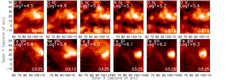
Figure 1: Intensity maps (on a logarithmic scale) of the lines listed in Table 1. The approximate time when the BP was scanned is shown in the lower right corner of each map.

In order to build up intensity maps and Dopplergrams for the lines listed in Table 1, we applied a single Gaussian fit to each spectral profile. Then we estimated the line shift caused by the thermal deformation of the optical system of SUMER, using a similar method as described in Dammasch et al. (1999). Also, the fitted center of an EIS line was further corrected by taking into account the slit-tilt effect and orbital variation of the line position. We assumed a vanishing Doppler shift for each line when being averaged over the whole FOV. In this way we could calibrate the wavelength and obtained a Dopplergram for each line. Fig. 1 and Fig. 2 show part of the resulting intensity maps and Dopplergrams, respectively.

During this time period, only the 96-min MDI (Michelson Doppler Imager) magnetograms (Scherrer et al., 1995) were available. Fig. 3 shows four magnetograms of the region in the vicinity of the BP taken at four different times. They were coaligned by using the SUMER continuum intensity image obtained around 750 Å. The right-most panel of Fig. 3 is the magnetic skeleton of the BP region projected onto the plane of the photosphere. We first used the YAFTA (Yet Another Feature Tracking Algorithm) software (Welsch et al., 2004; DeForest et al., 2007) to select all individual magnetic concentrations and then reduced them to point sources. With the help of the MPOLE (the Magnetic Charge Topology and Minimum Current Corona model) software (Longcope and Klapper, 2002), we could reconstruct the potential magnetic field topology produced by the set of point sources.

Some lines listed in Fig. 4 are weak or blended. However, by using the method of single or double gaussian fitting, we can still obtain a reliable intensity for each line in the BP region. Each of the density-sensitive line pairs was observed simultaneously. The theoretical relations between intensity ratios of line pairs and electron densities are shown in the top of Fig. 4 and were taken from the CHIANTI data base (Dere et al., 1997; Landi et al., 2006). Some blends discussed in Young et al. (2007) were also considered. We calculated intensities and densities for each individual pixel within the corresponding contoured region in Fig. 2 and then averaged those densities. We should mention that the O iv line pair was observed at about 11:40, when the BP was still there. The results are shown in the bottom of Fig. 4.

3 Results and discussion

The temperature dependence of the emission of BPs and their different plasma properties at different wavelengths are not yet well understood. Most of the previous studies concentrated on BPs as seen in only one wavelength or band. Few authors have analyzed a BP seen simultaneously at different temperatures (Habbal and Withbroe, 1981; Habbal et al., 1990; Habbal and Grace, 1991; Ugarte-Urra et al., 2004; McIntosh, 2007; Brosius et al., 2007).

Our Fig. 1 reveals the rich morphology of a BP when observed with such a wide temperature coverage. The Dopplergrams and related intensity contours are shown in Fig. 2. It is believed that BPs can experience variations in emission intensity and Doppler shift on a time scale of minutes (Habbal et al., 1990; Madjarska et al., 2003). However, the general emission pattern of some BPs can remain almost the same for 1-3 hours (see Fig. 2 in Brown et al. (2001)). We should not exclude the possibility of the presence of a more or less stable component of emission and Doppler flow in some BPs. In our case, the orientation and Doppler pattern (especially the sharp boundary between patches of red and blue shift) of the BP are both different at higher ($\log(T/\rm{K})>5.7$) and lower ($\log(T/\rm{K})<5.7$) temperatures. At lower temperatures, although the BP was observed at different times from 02:19 to 04:05, its orientation and Doppler pattern seem to be consistent and do not change too much.

Recently, Brosius et al. (2007) found Doppler shifts on opposite sides of a BP ranging from $-15$ to $+15$ km/s in He ii, and from $-35$ to $+35$ km/s in Fe xvi. Our results demonstrate that the Doppler shifts in the BP are quite different in different lines. Patches of red and blue shift are both found in the BP with comparable sizes. The absolute shift is largest in middle-transition region lines ($\log(T/\rm{K})=4.9-5.2$) and can reach more than 10 km/s.

The most interesting phenomenon visible in Fig. 2 is that the boundary between up/down flows in the BP is totally different, i.e. almost perpendicular, for lines with lower and higher temperatures. This boundary in Ne viii resembles those of lines with a higher temperature. But the Doppler pattern of Ne viii is similar to those of lines with a lower temperature in the surrounding quiet Sun. McIntosh (2007) classified the BPs seen in He ii (304 Å) and soft X-ray as cool and hot BPs, respectively. Similarly, we define here the bright feature seen at coronal temperature as the hot component, and the corresponding bright emission at TR temperature as the cool component of a BP. Considering the morphology and Doppler pattern of the BP, we found that a transition from the cool to the hot component of the BP occurs at a temperature of about $\log(T/\rm{K})=5.7$.

The different boundary between up/down flows at lower and higher temperatures in the BP might be a result of a syphon flow along a twisted loop system, which twists or spirals at its upper segment. Then the flow may lead to comparable red and blue shifts in the opposite legs, and result in a different boundary of the up and down flows located between the lower and upper parts of the loop. In Fig. 3, we found that the main negative magnetic source rotated relative to the positive source in a right-hand sense during the time period from 00:03 to 09:39. This movement might indicate a continual twist of the entire loop system. We have applied the force-free magnetic field extrapolation technique (Seehafer, 1978) to reconstruct the 3-D magnetic field in our BP region, but we could not reconstruct such a helical loop system. This does not mean that the twisted loop is not there, because the BP may simply not be a force-free structure, and consequently the extrapolation used may not represent the real magnetic field adequately. However, the up and down flows in our case might also be associated with magnetic reconnection as discussed in Brosius et al. (2007).

The different emission morphology and Doppler pattern between the cool and hot components of the BP may imply a different powering mechanism of the two components. McIntosh (2007) proposed a two-stage heating process, in which magnetoconvection-driven reconnection occurs in and supplies energy to the cool BPs, whereupon the increased energy supply leads to an expansion of the loop system, which interacts with the overlying coronal magnetic flux through fast separator reconnection and produces hot BPs. From magnetograms taken before and after the observation periods of SUMER and EIS, we find that the main negative source in the left frames of Fig. 3 is seen to approach and partly cancel the positive source. This cancellation might have started before, and still be in process after our spectroscopic observations. We also find that the three separators (A4-B1,A4-B2,A4-B3) in the magnetic skeleton at 04:51 partly fit the orientation of the hot component of the BP. Thus, our observations seem to support the two-stage powering mechanism.

The electron density is vital to determine the radiative losses in coronal heating models. Here we derived separately the densities of the cool and hot components of the same BP. The results are summarized in Fig. 4. Our derived values of the electron density in the range from $\log(T/\rm{K})=6.1$ to $6.3$ are similar to those of Ugarte-Urra et al. (2005) and Brosius et al. (2008). These densities are in the range of values typical of ARs, and slightly larger than quiet-Sun densities. The result of the higher value obtained with Fe xii compared to Si x is nothing new and a related discussion can be found in Ugarte-Urra et al. (2005).

The densities of the cool component of the BP have large uncertainties. But they can still be considered to be much higher than the density of the normal quiet Sun, which has an upper limit of $\log(N_{e}/\rm{cm}^{-3})=9.87$ at $\log(T/\rm{K})=5.25$ in Griffiths et al. (1999). Tripathi et al. (2008) derived a density of $\log(N_{e}/\rm{cm}^{-3})=10.0-10.5$ at $\log(T/\rm{K})=5.8-6.1$ inside the moss region of an AR. If we assume the density decreases with increasing temperature in the transition region, we can expect an even higher density of the AR at $\log(T/\rm{K})=5.2-5.4$. It should be comparable to, or larger than, our derived densities at $\log(T/\rm{K})=5.2-5.4$. So, the conclusion in Ugarte-Urra et al. (2005), namely that the BP plasma has more similarities to active-region than quiet-Sun plasma, may also be true for the cool component.

Table 1: Emission lines used to study the Doppler shifts of the BP. Here $\lambda$ and $T$ represent the rest wavelength and formation temperature, respectively.

SUMER lines			EIS lines
Ion	$\lambda$ (Å)	$\log(T/\rm{K})$	Ion	$\lambda$ (Å)	$\log(T/\rm{K})$
O ii	833.332	4.5	Fe viii	185.21	5.6
O iii	833.749	4.9	Fe x	184.54	6.0
S iv	750.221	5.0	Fe xii	195.12	6.1
N iv	765.148	5.1	Fe xiii	202.04	6.2
O iv	787.711	5.2	Fe xiv	264.79	6.3
O v	758.677	5.4
Ne viii	770.428	5.8

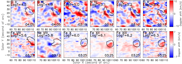
Figure 2: Dopplergrams of the lines listed in Table 1. The approximate time when the BP was scanned is shown in the lower right corner of each map. The black contours outline the positions of the BP as seen in different wavelengths.

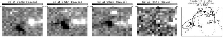
Figure 3: From left to right: MDI magnetograms taken at 00:03, 04:51, 09:39, 19:12, and the magnetic skeleton at 04:51. The FOV corresponds to a coordinate range of x from $80^{\prime\prime}$ to $115^{\prime\prime}$, and of y from $5^{\prime\prime}$ to $37^{\prime\prime}$. In the magnetic skeleton, positive/negative magnetic point sources are labelled P/N and marked with plus/cross symbols; positive/negative nulls are labelled B/A and marked with triangles pointing down/up; spines and separators are shown as dotted and solid lines,respectively; dashed lines indicate where separatrix surfaces intersect the photosphere.

Figure 4: Top: The theoretical relation between the intensity ratios of 6 line pairs and the corresponding electron densities. Bottom: The derived electron densities and their uncertainties indicated by standard deviation bars.

References

- Brosius et al. (2007) Brosius, J. W., Rabin, D. M., & Thomas, R. J. 2007, ApJ, 656, L41
- Brosius et al. (2008) Brosius, J. W., Rabin, D. M., Thomas, R. J., & Landi, E. 2008, ApJ, 677, 781
- Brown et al. (2001) Brown, D. S., et al. 2001, Sol. Phys., 201, 305
- Büchner (2006) Büchner, J. 2006, Space Science Reviews, 122, 149
- Culhane et al. (2007) Culhane, J.L. et al. 2007, Solar Phys., 243, 19
- Dammasch et al. (1999) Dammasch, I. E., Wilhelm, K., Curdt, W.,& Hassler, D. M. 1999, A&A, 346, 285
- DeForest et al. (2007) DeForest, C. E., et al. 2007, ApJ, 666, 576
- Dere et al. (1997) Dere, K. P., et al. 1997, A&AS, 125, 149
- Gabriel (1976) Gabriel A. H. 1976, Philos. Trans. R. Soc. London A, 281, 575
- Falconer et al. (1998) Falconer, D. A., Moore, R. L., Porter, J. G., & Hathaway, D. H. 1998, ApJ, 501, 386
- Golub et al. (1974) Golub, L., et al. 1974, ApJ, 189, L93
- Griffiths et al. (1999) Griffiths, N. W., Fisher, G. H., Woods, D. T., & Siegmund,O. H. W. 1999, ApJ, 512,992
- Habbal and Withbroe (1981) Habbal, S. R., & Withbroe, G. L. 1981, Sol. Phys., 69, 77
- Habbal et al. (1990) Habbal. S. R., Dowdy, J. F. Jr., &Withbroe, G. L. 1990, ApJ, 352,333
- Habbal and Grace (1991) Habbal, S. R., & Grace, E. 1991, ApJ, 382, 667
- Landi et al. (2006) Landi, E., et al. 2006, ApJS, 162, 261
- Lemaire et al. (1997) Lemaire P., Wilhelm K., Curdt W., et al. 1997, Sol. Phys., 170,105
- Longcope (1998) Longcope, D. W. 1998, ApJ, 507, 433
- Longcope and Klapper (2002) Longcope, D. W. & Klapper, I. 2002, ApJ, 579, 468
- Madjarska et al. (2003) Madjarska, M. S., Doyle, J. G., Teriaca, L., & Banerjee, D. 2003, A&A, 398, 775
- McIntosh (2007) McIntosh, S. W. 2007, ApJ, 670, 1401
- Parnell et al. (1994) Parnell, C. E., Priest, Eric R., &Titov, V. S. 1994, Sol. Phys., 153, 217
- Priest et al. (1994) Priest, E. R., Parnell, C. E., &Martin, S. F. 1994, ApJ, 427, 459
- Santos and Büchner (2007) Santos, J. C., &Büchner, J., Astrophys. Space Sci. Trans. 2007, 3, 29
- Scherrer et al. (1995) Scherrer, P. H., et al. 1995, Solar Phys., 162,129
- Seehafer (1978) Seehafer, N. 1978, Sol. Phys., 58, 215
- Sheeley and Golub (1979) Sheeley, N. R. Jr., & Golub, L. 1979, Sol. Phys., 63, 119
- Tian et al. (2007) Tian H., Tu C.-Y., He J.-S., &Marsch, E. 2007, Adv. Space Res., 39,1853
- Tian et al. (2008) Tian H., Marsch E., Tu C.-Y., Xia L.-D., &He J.-S. 2008, A&A, 482,267
- Tripathi et al. (2008) Tripathi, D., Mason, H. E., Young, P. R., & Del Zanna, G. 2008, A&A 481, L53
- Ugarte-Urra et al. (2004) Ugarte-Urra, I., Doyle, J. G., Madjarska, M. S., & O′Shea, E. 2004, A&A, 418, 313
- Ugarte-Urra et al. (2005) Ugarte-Urra, I., Doyle, J. G., & Del Zanna G. 2005, A&A, 435, 1169
- Von Rekowski et al. (2006) Von Rekowski B., Parnell, C. E., &Priest, E. R. 2006, MNRAS, 366, 125
- Webb et al. (1993) Webb, D. F., Martin, S. F., Moses, D., & Harvey, J. W. 1993, Sol. Phys., 144, 15
- Welsch et al. (2004) Welsch, B. T., Fisher, G. H., Abbett, W. P., & Regnier, S. 2004, ApJ, 610, 1148
- Wilhelm et al. (1995) Wilhelm K., Curdt W., Marsch E., et al. 1995, Sol. Phys., 162,189
- Xia et al. (2003) Xia, L. D., Marsch, E., & Curdt, W. 2003, A & A, 399, L5
- Xia (2003) Xia, L.-D. 2003, Ph.D. Thesis (Göttingen: Georg-August-Univ.)
- Young et al. (2007) Young,P. R., et al. 2007, PASJ, 59, S857
- Zhang et al. (2001) Zhang, J., Kundu, M. R., & White, S. M. 2001, Sol. Phys., 198, 347