Long-range multiplicity correlations in
proton-proton collisions

Abstract

The forward-backward long-range multiplicity correlations in proton-proton collisions are investigated in the model with two independent sources of particles: one left- and one right-moving wounded nucleon. A good agreement with the UA5 collaboration proton-antiproton data at the c.m. energy of $200$ GeV is observed. For comparison the model with only one source of particles is also discussed.

PACS: 25.75.Gz, 13.85.Hd
Keywords: pp, forward-backward correlations, wounded nucleon

1 Introduction

Recently, the pseudorapidity particle density from a wounded nucleon was determined by analysing the PHOBOS data [2] on deuteron-gold collisions at $\sqrt{s}=200$ GeV in the framework of the wounded nucleon [3] and the wounded quark-diquark [4] models. The obtained fragmentation function has two characteristic features. It is peaked in the forward direction and it substantially feeds into the opposite hemisphere, as shown in Fig. 1. In Ref. [6] very similar shape of the contribution from a wounded nucleon was found at SPS energy of $\sqrt{s}=17.3$ GeV. The possible explanation of the main features of the wounded nucleon fragmentation function was proposed in Ref. [7] in the model based on the bremsstrahlung mechanism [8].

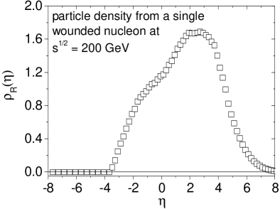
Figure 1: The pseudorapidity density of produced charged particles from a right-moving wounded nucleon at $\sqrt{s}=200$ GeV c.m. energy. $\rho_{R}(\eta)$ substantially feeds into the opposite hemisphere which implies specific long-range forward-backward multiplicity correlations.

It is interesting to notice that the picture in which the wounded nucleon populates particles into the opposite hemisphere implies specific long-range forward-backward multiplicity correlations. This problem will be investigated here in the context of the UA5 $p\bar{p}$ forward-backward multiplicity correlation data at $\sqrt{s}=200$ GeV [9]. Namely, we will test the model with two independent sources of particles, see Fig. 2, with the wounded nucleon fragmentation function shown in Fig. 1. For comparison, we will also study the model in which particles are produced from only one source of particles e.g., a single string spanned between two wounded nucleons.

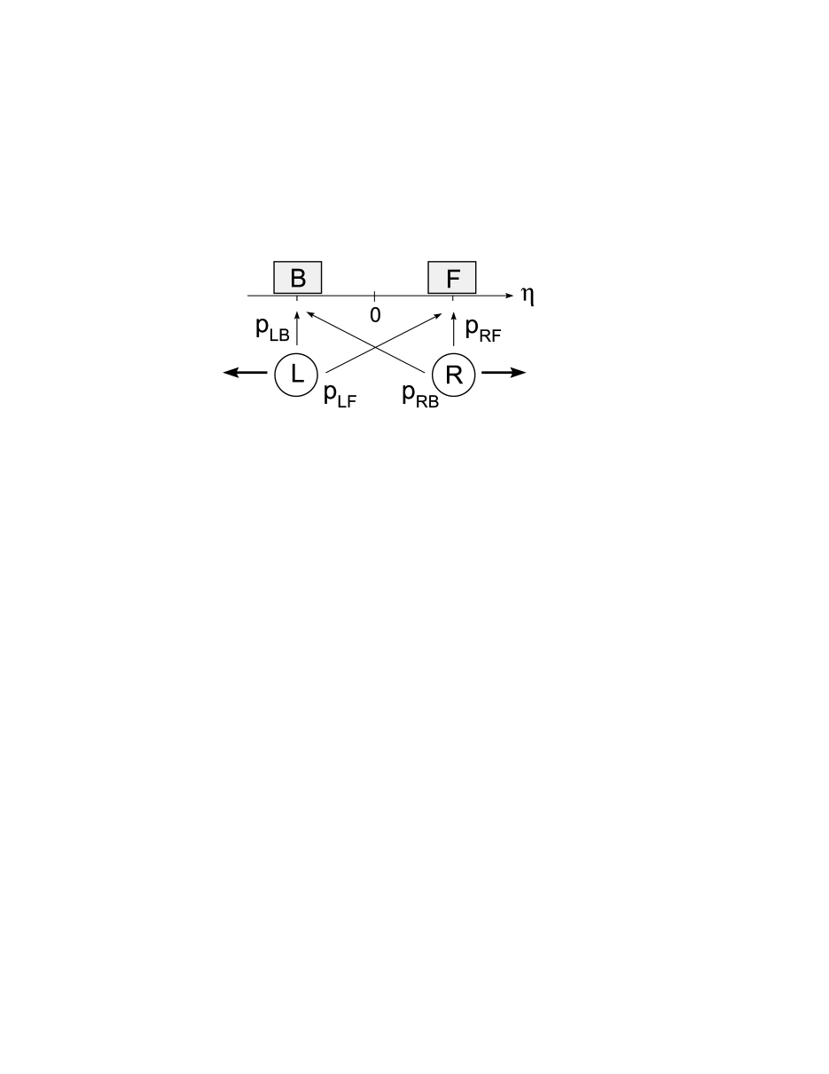
Figure 2: The model of soft particle production in proton-proton collisions with two independent sources of particles: left- and right-moving wounded nucleons. The arrows indicate that each wounded nucleon may populate particles into both pseudorapidity intervals with appropriate probabilities.

Our main conclusion is that the model with two independent sources of particles and the wounded nucleon fragmentation function extracted from the PHOBOS $d-Au$ data is fully consistent with the UA5 $p\bar{p}$ forward-backward multiplicity correlation data at $\sqrt{s}=200$ GeV. At the same time we conclude that the model with only one source of particles is in a very clear disagreement with the data.

Let us emphasize here that the idea of the multicomponent model of soft particle production is not new and was successfully applied to the forward-backward multiplicity correlations data by many authors [5, 10, 11, 12, 13, 14, 15]. Our model with two sources of particles has very much in common with the dual parton model [5] or the two-chain dual model with non-zero asymmetry of each chain [10, 11]. For other approaches see Refs. [16, 17].

In the next section basic formulae are introduced. In section $3$ we present our model in detail and derive for $pp$ collisions the analytical expressions for the correlation coefficient and the functional relation between the average number of particles in the backward interval at a given number of particles in the forward one. We also discuss the limit of one-source model. In section $4$ our results are tested using UA5 $p\bar{p}$ forward-backward multiplicity correlation data. Our conclusions are listed in the last section, where also some comments are included.

2 General formulae

It is convenient to construct the generating function

$$H\left(z_{B},z_{F}\right)=\sum\nolimits_{n_{B},n_{F}}P\left(n_{B},n_{F}\right)z_{B}^{n_{B}}z_{F}^{n_{F}},$$ (1)

where $P\left(n_{B},n_{F}\right)$ is the probability in $pp$ collisions to find $n_{B}$ particles in $B$ interval and $n_{F}$ particles in $F$ interval, see Fig. 2. It is worth to notice that the generating function (1) contains all information about the multiplicities in $B$ and $F$.

The correlation coefficient (or correlation strength) is defined as

$$b=\frac{\left\langle n_{B}n_{F}\right\rangle-\left\langle n_{B}\right\rangle\left\langle n_{F}\right\rangle}{\left\langle n_{F}^{2}\right\rangle-\left\langle n_{F}\right\rangle^{2}},$$ (2)

where $n_{B}$ and $n_{F}$ are event by event particle multiplicities in $B$ and $F$ intervals, respectively. If the number of particles in $B$ interval does not dependent on the number of particles in $F$ i.e., $\left\langle n_{B}n_{F}\right\rangle=\left\langle n_{B}\right\rangle\left\langle n_{F}\right\rangle$ we have $b=0$. On the other hand, if $n_{B}=n_{F}$ in every event then $b=1$ (maximum correlation). Using definition (1) the correlation coefficient $b$ can be expressed by the appropriate derivatives of the generating function

$$\left\langle n_{B}n_{F}\right\rangle-\left\langle n_{B}\right\rangle\left\langle n_{F}\right\rangle =\left[\frac{\partial^{2}H}{\partial z_{B}\partial z_{F}}-\frac{\partial H}{\partial z_{B}}\frac{\partial H}{\partial z_{F}}\right]_{z_{B}=1,z_{F}=1},$$

$$\left\langle n_{F}^{2}\right\rangle-\left\langle n_{F}\right\rangle^{2} =\left[\frac{\partial^{2}H}{\partial z_{F}^{2}}+\frac{\partial H}{\partial z_{F}}-\left(\frac{\partial H}{\partial z_{F}}\right)^{2}\right]_{z_{B}=1,z_{F}=1}.$$ (3)

It is also interesting to study the functional relation between the average number of particles $\left\langle n_{B}\right\rangle$ in $B$ interval under the condition of $n_{F}$ particles in $F$ interval

$$\left\langle n_{B}\right\rangle|_{n_{F}}=\frac{\sum\nolimits_{n_{B}}n_{B}P\left(n_{B},n_{F}\right)}{\sum\nolimits_{n_{B}}P\left(n_{B},n_{F}\right)},$$ (4)

where the numerator and denominator can be expressed by the derivatives of the generating function (1)

$$\sum\nolimits_{n_{B}}P\left(n_{B},n_{F}\right) =\left.\frac{1}{n_{F}!}\frac{\partial^{n_{F}}H\left(z_{B},z_{F}\right)}{\partial z_{F}^{n_{F}}}\right|_{z_{B}=1,z_{F}=0},$$

$$\sum\nolimits_{n_{B}}n_{B}P\left(n_{B},n_{F}\right) =\left.\frac{1}{n_{F}!}\frac{\partial}{\partial z_{B}}\frac{\partial^{n_{F}}H\left(z_{B},z_{F}\right)}{\partial z_{F}^{n_{F}}}\right|_{z_{B}=1,z_{F}=0}.$$ (5)

In the next section we calculate (2) and (4) in two models of particle production.

3 Model

The schematic view of our model is presented in Fig. 2. We assume that in $pp$ collisions all soft particles are produced from two independent wounded nucleons, which populate particles according to the fragmentation function presented in Fig. 1. Additionally, we assume that in $pp$ collisions the multiplicity distribution in the combined interval $B+F$ is described be the negative binomial (NB) distribution

$$P_{NB}(n,\bar{n},k)=\frac{\Gamma(n+k)}{\Gamma(n+1)\Gamma(k)}\left(\frac{\bar{n}}{k}\right)^{n}\left(1+\frac{\bar{n}}{k}\right)^{-n-k},$$ (6)

where $\bar{n}$ is the average multiplicity in $B+F$ and $1/k$ measures deviation from Poisson distribution. It is obvious that $\bar{n}$ can be calculated as

$$\bar{n}=\int_{B+F}\left[\rho_{R}\left(\eta\right)+\rho_{L}\left(\eta\right)\right]d\eta=2\int_{B+F}\rho_{R}\left(\eta\right)d\eta,$$ (7)

where $\rho_{R}\left(\eta\right)$ and $\rho_{L}\left(\eta\right)=\rho_{R}\left(-\eta\right)$ are the pseudorapidity densities of produced particles from the right- and left-moving wounded nucleons, respectively.

Recently, we have shown [18] that the generating function (1) in the framework of the above-mentioned model may be written as

$$H\left(z_{B},z_{F}\right) =\left\{1+\frac{\bar{n}}{k}\left[p_{LB}\left(1-z_{B}\right)+p_{LF}\left(1-z_{F}\right)\right]\right\}^{-k/2}\times$$

$$\times\left\{1+\frac{\bar{n}}{k}\left[p_{RB}\left(1-z_{B}\right)+p_{RF}\left(1-z_{F}\right)\right]\right\}^{-k/2},$$ (8)

where $p_{RF}$ is the probability that a particle originating from the right-moving wounded nucleon goes to $F$ interval rather than to $B$ (and analogous for $p_{RB},p_{LB}$ and $p_{LF}$), see Fig. 2. These probabilities satisfy the following conditions

$$p_{LB}+p_{LF}=1,\quad p_{RB}+p_{RF}=1.$$ (9)

These numbers can be easily calculated using the wounded nucleon fragmentation function. For instance, $p_{RF}$ has the form

$$p_{RF}=\frac{\int_{F}\rho_{R}\left(\eta\right)d\eta}{\int_{B+F}\rho_{R}\left(\eta\right)d\eta}.$$ (10)

Taking (2), (3) and (8) into account and performing elementary calculations, the following expression for the correlation coefficient in the model with two independent sources of particles is obtained

$$b=\frac{\bar{n}(p_{LB}p_{LF}+p_{RB}p_{RF})}{\bar{n}(p_{LF}^{2}+p_{RF}^{2})+k(p_{LF}+p_{RF})}.$$ (11)

Assuming that intervals $B$ and $F$ are separated enough so that $F$ can be populated only by the right-moving nucleon and $B$ only by the left-moving one i.e., $p_{LB}=p_{RF}=1$ and $p_{LF}=p_{RB}=0$ we obtain $b=0$. Thus, we immediately predict the noticeable suppression of the correlation coefficient $b$ with increasing distance between $B$ and $F$ intervals.

In the model with two independent sources of particles the relation between the average number of particles $\left\langle n_{B}\right\rangle$ in the backward interval $B$ at a given number of particles $n_{F}$ in the forward interval $F$ has the form [see (4), (5) and (8)]

$$\left\langle n_{B}\right\rangle|_{n_{F}} =\frac{k\bar{n}p_{LB}}{2\left(k+\bar{n}p_{LF}\right)}\frac{{}_{2}F_{1}(1+k/2,-n_{F},1-n_{F}-k/2,\xi)}{{}_{2}F_{1}(k/2,-n_{F},1-n_{F}-k/2,\xi)}+$$

$$+\frac{\bar{n}p_{RB}\left(n_{F}+k/2\right)}{k+\bar{n}p_{RF}}\frac{{}_{2}F_{1}(k/2,-n_{F},-n_{F}-k/2,\xi)}{{}_{2}F_{1}(k/2,-n_{F},1-n_{F}-k/2,\xi)},$$ (12)

where

$$\xi=\frac{p_{LF}(k+\bar{n}p_{RF})}{p_{RF}(k+\bar{n}p_{LF})},$$ (13)

and the hypergeometric function ${}_{2}F_{1}(a,-n_{F},1-c,\xi)$ is defined as

$${}_{2}F_{1}(a,-n_{F},1-c,\xi)=\frac{\Gamma(1+n_{F})}{\Gamma(a)\Gamma(c)}\sum\limits_{M=0}^{n_{F}}\frac{\Gamma(a+M)\Gamma(c-M)}{M!(n_{F}-M)!}\xi^{M}.$$ (14)

For comparison we also derive the appropriate formulae in the model with only one source of particles e.g., a single string spanned between two wounded nucleons. These expressions can be easily obtained from (11) and (12) by deactivating one of the sources e.g., the left one. In this case $p_{LB}=p_{LF}=0$ (thus $\xi=0$) and $p_{RB}\equiv p_{B}$ and $p_{RF}\equiv p_{F}$ where $p_{B}+p_{F}=1$. Finally

$$b=\frac{p_{B}\bar{n}}{k+p_{F}\bar{n}},$$ (15)

and

$$\left\langle n_{B}\right\rangle|_{n_{F}}=\frac{p_{B}\bar{n}}{k+p_{F}\bar{n}}\left(\frac{k}{2}+n_{F}\right).$$ (16)

This closes the theoretical discussion of the problem.

4 Results

In the present section we test our results using the UA5 $p\bar{p}$ forward-backward multiplicity correlation data at $\sqrt{s}=200$ GeV. The measurement was performed in the pseudorapidity range of $|\eta|<4$ for various symmetric (around $\eta=0$) forward and backward intervals. In this case, taking the model with two independent sources, we have $p_{RF}=p_{LB}\equiv p$ and $p_{RB}=p_{LF}=1-p$, where probability $p$ is calculated from Eq. (10). In the model with only one source we always have $p_{B}=p_{F}=1/2$.

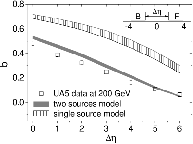
Figure 3: The forward-backward multiplicity correlation coefficient $b$ as a function of the distance $\Delta\eta$ between the backward $B$ and forward $F$ intervals. Data points (squares) measured in $p\bar{p}$ at $\sqrt{s}=200$ GeV are compared with the results of two models: two independent sources of particles (grey band) and the model with a single source (dashed band). The widths of the bands reflect the uncertainty in the value of $k$ from NB fits to the $p\bar{p}$ multiplicity data.

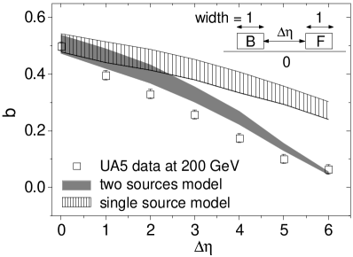
Figure 4: The same as in Fig. 3 but now the width of each interval is fixed and equals $1$.

In Figs. 3 and 4 the correlation coefficient $b$ for various symmetric pseudorapidity intervals is presented. The experimental data (squares) are taken from Refs. [9, 19]. The grey and dashed bands represent the results of the model with two independent sources and the model with a single source, respectively. The widths of the bands reflect the uncertainty coming from the unknown precise value of $k$ from NB distribution fits [20] to the $p\bar{p}$ multiplicity data. In Fig. 3 the forward and backward intervals are chosen as: $B=(-4,-\Delta\eta/2)$ and $F=(\Delta\eta/2,4)$ with $\Delta\eta=0,1,2,3,4,5,6$. In Fig. 4 the forward and backward intervals of constant widths of $1$ are: $B=(-\Delta\eta/2-1,-\Delta\eta/2)$ and $F=(\Delta\eta/2,\Delta\eta/2+1)$. The parameters $p$ and $\bar{n}$ are calculated using Eqs. (10), (7) and the wounded nucleon fragmentation function shown in Fig. 1. All parameters used in these calculations are listed in Tabs. 1 and 2. In both cases the main source of uncertainties is the NB parameter $k$, which is not precisely known for all intervals [20].

As can be observed the model with two independent sources of particles allows to understand the main features of the data. It is worth noticing that the strong suppression of the correlation coefficient $b$ with increasing $\Delta\eta$ is fully determined by the suppression of particle production from a single wounded nucleon to the backward hemisphere. Clearly, the model in which particles are produced from the single source is incorrect.

$\Delta\eta$	$F$ interval	$\bar{n}$	$k$	$p$
$0$	$0.0<\eta<4.0$	$17.4$	$3.70\pm 0.30$	$0.70$
$1$	$0.5<\eta<4.0$	$15.1$	$3.85\pm 0.35$	$0.73$
$2$	$1.0<\eta<4.0$	$12.6$	$3.95\pm 0.40$	$0.76$
$3$	$1.5<\eta<4.0$	$10.2$	$4.10\pm 0.50$	$0.80$
$4$	$2.0<\eta<4.0$	$7.71$	$4.25\pm 0.55$	$0.84$
$5$	$2.5<\eta<4.0$	$5.39$	$4.35\pm 0.60$	$0.89$
$6$	$3.0<\eta<4.0$	$3.30$	$4.50\pm 0.70$	$0.94$

Table 1: The parameters used in the calculations of the results presented in Fig. 3.

$\Delta\eta$	$F$ interval	$\bar{n}$	$k$	$p$
$0$	$0.0<\eta<1.0$	$4.76$	$2.30\pm 0.30$	$0.54$
$1$	$0.5<\eta<1.5$	$4.88$	$2.70\pm 0.40$	$0.59$
$2$	$1.0<\eta<2.0$	$4.94$	$3.05\pm 0.45$	$0.64$
$3$	$1.5<\eta<2.5$	$4.78$	$3.40\pm 0.50$	$0.70$
$4$	$2.0<\eta<3.0$	$4.41$	$3.80\pm 0.60$	$0.76$
$5$	$2.5<\eta<3.5$	$3.90$	$4.10\pm 0.60$	$0.85$
$6$	$3.0<\eta<4.0$	$3.30$	$4.50\pm 0.70$	$0.94$

Table 2: The parameters used in the calculations of the results presented in Fig. 4.

In Fig. 5 the relation $\left\langle n_{B}\right\rangle|_{n_{F}}$ between the average number of particles $\left\langle n_{B}\right\rangle$ in $B$ interval at a given number of particles $n_{F}$ in $F$ interval is shown. The measurement was performed in two symmetric pseudorapidity intervals $B=(-4,0)\$and $F=(0,4)$. Taking Eqs. (10), (7) into account we obtain $p=0.7$ and $\bar{n}=17.4$. The main source of uncertainties is the measured value of $k=3.7\pm 0.3$ [20].

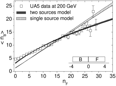
Figure 5: The relation between the average number of particles in the backward interval $\left\langle n_{B}\right\rangle$ at a given number of particles $n_{F}$ in the forward one. The UA5 $p\bar{p}$ experimental data (squares) at $\sqrt{s}=200$ GeV are compared with the results of the model with two independent sources of particles (grey band) and the model with a single source (dashed band). The widths of the bands reflect the uncertainty in the value of $k$ from NB fits to the $p\bar{p}$ multiplicity data.

The model with two independent sources of particles again correctly describes the data. It is interesting to note that our formalism predicts some deviations from linearity, which are too small to be noticeable at a given experimental precision.

5 Conclusions and comments

Our conclusions can be formulated as follows.

(i) Assuming that in $pp$ collisions soft particles are produced from two independent sources: left- and right-moving wounded nucleons, we have derived the formulae for the forward-backward multiplicity correlation coefficient $b$ and the functional relation between the average number of particles in the backward interval $\left\langle n_{B}\right\rangle$ at a given number of particles $n_{F}$ in the forward one. This is compared with the case where only one source contributes to particle spectrum.

(ii) We compared our results with the UA5 $p\bar{p}$ data at $\sqrt{s}=200$ GeV. We conclude that the model with two independent sources of particles allows to understand the main features of the forward-backward correlation data. As far as the correlation coefficient is concerned, we observed very nice qualitative agreement, particularly linear suppression of $b$ with increasing distance between the forward and backward intervals. This effect is fully determined by the suppression of the particle production from a wounded nucleon to the backward hemisphere.

(iii) We also successfully described the functional relation of the average number of particles in the backward interval $\left\langle n_{B}\right\rangle$ at a given number $n_{F}$ of particles in the forward one. It is interesting to note that our formalism predicts some deviations from linearity, which are too small to be noticeable at a given experimental precision. It would be interesting to study this effect in the future experiments.

(iv) The model in which the particles are produced from a single source is in a clear disagreement with the data.

Following comments are in order.

(a) The presented analysis was performed only at $\sqrt{s}=200$ GeV since for higher energies the wounded nucleon fragmentation functions are unknown. Studying the correlation data at higher energies should allow to extract these functions.

(b) Assuming $\left\langle n_{B}\right\rangle|_{n_{F}}$ to be in the parabolic form with the quadratic term $n_{F}^{2}c$ in the range $n_{F}<40$ and $n_{F}<50$ we obtained $c\approx-0.0045$ and $-0.0035$, respectively. It is interesting to note that qualitatively similar tendency was observed in the quantum-statistical approach [21].

Acknowledgements

We would like to thank Andrzej Białas for suggesting this investigation and useful discussions. This investigation was supported in part by the Polish Ministry of Science and Higher Education, grant No. N202 034 32/0918.

References

- [1] A. Bialas, M. Bleszynski and W. Czyz, Nucl. Phys. B111 (1976) 461.
- [2] PHOBOS Collaboration: B.B. Back et al., Phys. Rev. C72 (2005) 031901.
- [3] A. Bialas and W. Czyz, Acta Phys. Polon. B36 (2005) 905.
- [4] A. Bialas and A. Bzdak, Phys. Rev. C77 (2008) 034908; Phys. Lett. B649 (2007) 263; Acta Phys. Polon. B38 (2007) 159. For a review, see A. Bialas, J. Phys. G35 (2008) 044053.
- [5] A. Capella, U. Sukhatme, C-I Tan and J. Tran Thanh Van, Phys. Rept. 236 (1994) 225.
- [6] G. Barr, O. Chvala, H.G. Fischer, M. Kreps, M. Makariev, C. Pattison, A. Rybicki, D. Varga and S. Wenig, Eur. Phys. J. C49 (2007) 919; A. Rybicki, Acta Phys. Polon. B33 (2002) 1483.
- [7] A. Bialas, A. Bzdak and R. Peschanski, Phys. Lett. B665 (2008) 35.
- [8] L. Stodolsky, Phys. Rev. Lett. 28 (1972) 60.
- [9] UA5 Collaboration: R.E. Ansorge et al., Z. Phys. C37 (1988) 191.
- [10] K. Fialkowski and A. Kotanski, Phys. Lett. B115 (1982) 425; Phys. Lett. B107 (1981) 132.
- [11] J. Dias de Deus, Phys. Lett. B100 (1981) 177.
- [12] J. Benecke, A. Bialas and S. Pokorski, Nucl. Phys. B110 (1976) 488, Erratum-ibid. B115 (1976) 547.
- [13] A. Giovannini and R. Ugoccioni, Phys. Rev. D66, (2002) 034001; Phys. Lett. B558 (2003) 59.
- [14] M.A. Braun, C. Pajares and V.V. Vechernin, Phys. Lett. B493 (2000) 54.
- [15] P. Brogueira, J. Dias de Deus and C. Pajares, arXiv:0901.0997 [hep-ph].
- [16] T.T. Chou and C.N. Yang, Phys. Lett. B135 (1984) 175.
- [17] S.L. Lim, Y.K. Lim, C.H. Oh and K.K. Phua, Z. Phys. C43 (1989) 621; S.L. Lim, C.H. Oh and K.K. Phua, Z. Phys. C54 (1992) 107.
- [18] A. Bzdak, arXiv:0902.2639 [hep-ph].
- [19] NA22 Collaboration: V.V. Aivazyan et al., Z. Phys. C42 (1989) 533.
- [20] UA5 Collaboration: R.E. Ansorge et al., Z. Phys. C43 (1989) 357.
- [21] G.N. Fowler, E.M. Friedlander, F.W. Pottarg, R.M. Weiner, J. Wheeler and G. Wilk, Phys. Rev. D37 (1988) 3127.