Finite-Dimensional Turbulence of Planetary Waves

Abstract

Finite-dimensional wave turbulence refers to the chaotic dynamics of interacting wave ‘clusters’ consisting of finite number of connected wave triads with exact three-wave resonances. We examine this phenomenon using the example of atmospheric planetary (Rossby) waves. It is shown that the dynamics of the clusters is determined by the types of connections between neighboring triads within a cluster; these correspond to substantially different scenarios of energy flux between different triads. All the possible cases of the energy cascade termination are classified. Free and forced chaotic dynamics in the clusters are investigated: due to the huge fluctuations of the energy exchange between resonant triads these two types of evolution have a lot in common. It is confirmed that finite-dimensional wave turbulence in finite wave systems is fundamentally different from kinetic wave turbulence in infinite systems; the latter is described by wave kinetic equations that account for interactions with overlapping quasi-resonances of finite amplitude waves. The present results are directly applicable to finite-dimensional wave turbulence in any wave system in finite domains with 3-mode interactions as encountered in hydrodynamics, astronomy, plasma physics, chemistry, medicine, etc.

I Introduction

I.1 Weak-wave turbulence in finite-size systems

“Wave turbulence” refers to the chaotic dynamics of nonlinearly coupled oscillatory modes. The phenomenon appears in a variety of physical context from surface water waves, through atmospheric planetary waves, plasma waves, acoustic waves in solids and fluids etc. Depending on the strength of nonlinear interaction one distinguishes weak-wave turbulence from strong-wave turbulence. Weak-wave turbulence is characterized by a smallness parameter $\zeta$ which is roughly the root mean square of the ratio of the nonlinear to the linear term in the equation of motion. For surface waves $\zeta$ is about the ratio of the wave amplitude to the wave-length $\lambda$, for sound in continues media this is the ratio of the density variations to the mean density, etc.

The theory of weak-wave turbulence is particularly well developed in the limit of infinite systems where the ratio of the system size $L$ to the characteristic wave length $\lambda$ is very large, $L/\lambda\to\infty$. In that limit the observed energy spectrum (energy distribution between modes) is well described by the so called “wave kinetic equations” that received considerable attention in the last half century, see e.g. ZLF ; NazarLvov2004 ; NazarLvov2005 ; NazarLvov2006 ; NewellZakhar2008 . We will call this regime of weak wave turbulence “kinetic wave turbulence” to distinguish it from other regimes, “finite-dimensional wave turbulence” and “mesoscopic wave turbulence” that will be introduced later.

Notice that when the parameter $L/\lambda$ is of the order of unity the dynamics of waves can be very well described by low-dimensional chaotic models of the type studied intensively in recent decades , see e.g. KL-07 ; KL-08 . In this paper we explore the non-linear dynamics of weakly interacting waves when the parameter $L/\lambda$ is neither of order unity nor very large. This regime of parameters cannot be described either by kinetic equations or as low-dimensional chaos; it calls for new approaches and novel concepts, as partially demonstrated in this paper.

To clarify the possible new regimes of weak-wave turbulence in various finite-domain systems we consider the general mathematical framework that takes the form of an energy conserving partial differential nonlinear equation for a field $\Psi({\bm{r}},t)$. In a finite domain $S$ one expands $\Psi({\bm{r}},t)$ in a complete set of eigenfunctions $\Phi_{j}({\bm{r}})$ of the linearized dynamics that satisfy the boundary condition on the boundary $\partial S$:

$$\Psi({\bm{r}},t)=\sum_{j}A_{j}(t)\Phi_{j}({\bm{r}})\ ,$$ (1)

where in general $j$ can be a multiple index and the amplitudes $A_{j}(t)$ are functions of time but not of space. Accordingly the dynamics can be represented by a set of ordinary differential equations for the vector of amplitudes ${\bm{A}}(t)=\{A_{j}(t)\}$, of the form

$$\frac{dA_{j}(t)}{dt}=i\omega_{j}A_{j}(t)+\mbox{NL}_{j}({\bm{A}})$$ (2)

where $\omega_{j}$ is the (real) eigenfrequency of the $j$th mode; The symbolic term NL stands for the nonlinear contributions in this equation. According to the Poincaré and Poincaré-Dulac theorems Arnold the nonlinear contributions can be brought to a normal form by a nonlinear change of variables. The nonlinear monomials that survive the change of variable are the resonant ones. The $n$-tuple $(\omega_{1},\dots\omega_{n})$ of eigenfrequencies is said to be resonant if there exists a relation of the form

$$\omega_{j}=m_{1}\omega_{1}+m_{2}\omega_{2}+\dots m_{n}\omega_{n}\ .$$ (3)

The order of the resonance is $\sum_{k}m_{k}$. The resonant monomials are of the form $A_{1}^{m_{1}}\dots A_{n}^{m_{n}}$.

For the case of weak nonlinearities we invoke the smallness parameter $\zeta\ll 1$ to discard all the higher order resonances, keeping only the lowest available order. In other words, if there exist solutions to the equation

$$\omega_{j}=\omega_{m}+\omega_{n}\ ,$$ (4a)

we keep only the resulting quadratic monomials also known as “three-wave interactions”, which satisfy the conservation law (4a). For example, in space-homogeneous, scale-invariant, isotropic, infinite wave-systems, in which the dependence of the wave frequency $$\omega(k) k\equiv|{\bm{k}}| \omega(k)\propto k^{\alpha}$$ on the wave vector , , the three wave resonances

$$\omega(k_{1})+\omega(k_{2})=\omega(|{\bm{k}}_{1}+{\bm{k}}_{2}|)\,,$$ (4b)

are allowed if $\alpha\geq 1$ ZLF . For $\alpha<1$ Eq. (4b) has no solutions and one needs to account for higher order resonances.

In this paper we focus on problems for which Eq. (4a) has solutions, determining the leading nonlinearity. We note that as the ratio $L/\lambda$ increases, there may be more and more eigenfrequencies that satisfy equation (4a). In particular, while at small values of $L/\lambda$ we can expect only isolated resonant triads of waves, for larger values of $L/\lambda$ triads can share a common mode and the number of coupled resonant triads increases considerably, finally forming infinite clusters of connected triads. Analysis of the ensuing dynamics under the influence of such growing clusters is the main subject of the present paper. We will focus here on the case of small enough nonlinearity parameter $\zeta$ to ensure that only waves with exact resonances are important. In this case one can consider only clusters of connected resonant triads of interacting waves. We will refer to the chaotic dynamics of interacting waves in this regime as “finite-dimensional wave turbulence”, to stress the importance of the finite number of interacting modes with exact wave resonances. With increasing of wave amplitudes one has to account also for quasi-resonances. This type of wave turbulence was called “discrete wave turbulence” Kar-06 . In contrast, in infinite systems, the resonance conditions [e.g. Eq. (4b)] has infinitely many solutions; then usually the (kinetic) wave turbulence can be described by wave kinetic equations. A more detailed analysis Naz-07 shows that in the plane ($L/\lambda\,,\zeta$) there exists a region of parameters where there exists weak-wave turbulence whose properties are intermediate between finite-dimensional and kinetic regimes. Some features of this type of turbulence, called “mesoscopic wave-turbulence”, were observed, for example, in NazarLvov2006 ; Zakhar2006 .

To study finite-dimensional wave turbulence we focus here for concreteness on the example of the barotropic vorticity equation on a sphere; this is an idealized model for atmospheric planetary (Rossby) waves ped , shortly described in Sec. II. Planetary-scale motions in the ocean and atmosphere are due to the shape and rotation of the Earth, and play a crucial role in weather and climate predictability ped . Oceanic planetary waves influence the general large-scale ocean circulation, can intensify the currents such as the Gulf Stream, as well as push them off their usual course. For example, a planetary wave can push the Kuroshio Current northwards and affect the weather in North America Kuroshio . Atmospheric planetary waves detach the masses of cold or warm air that become cyclones and anticyclones and are responsible for day-to-day weather patterns at mid-latitudes smth .

Recently a new model KL-07 was developed for the intra-seasonal oscillations in the Earth atmosphere, in terms of triads of planetary waves whose eigen-frequencies solve Eq. (4a). The study of the complete cluster structure in various spectral domains shows that both for atmospheric KK-07 and oceanic all-08 planetary waves indeed the size of the clusters increases with the growth of the spectral domain. In large clusters one finds both large and small wavenumbers, meaning that the energy flux between very different scales becomes possible, bringing with it the hallmark of turbulence. Nevertheless, both numerical simulations zak4 ; T07 and laboratory experiments DLN06 indicate that the dynamics of wave systems with intermediate value of $L/\lambda$ do not obey the statistical description provided by wave kinetic equations. This domain calls for a specialized investigation which is initiated in this paper.

I.2 Structure of this paper

Section II reviews the properties of atmospheric planetary waves which are important for our analyis: in Sec. II.1 we consider barotropic vorticity Eq. (II.1) on a sphere and its dynamical invariants (6); in Sec. II.2 we project Eqs. (II.1) and (6) on the spherical basis; and in Sec. II.3 we analyze the properties of the resulting interaction coefficients.

In Sections III and IV we study the topology and other properties of finite size clusters of resonant triads of planetary waves that influence the dynamics of finite-dimensional wave turbulence. In Sec. III we begin with small clusters of resonant triads. In Sec. III.1 we overview equation of motion (14) for isolated resonant triad and its dynamical invariants (15), present them in the Hamiltonian form (20), and use the notion of “active” and “passive” modes KL-08 denoted as A- and P-modes; these notions are crucial for our theory. In the next Sec. III.2 we move on to double-triad clusters, PP-, PA- and AA-butterflies, their Hamiltonian equation of motion (25), Hamiltonian (26) and Manley-Rowe dynamical invariants (27). Similar discussion for the triple-triad clusters, stars, chains and triangles, is given in Sec. III.3. Specific for atmospheric planetary waves, 6-triad cluster, caterpillar, is presented in Sec. III.4 as an example of a more complicated cluster structure.

In Sec. IV we study clusters of atmospheric planetary waves in a large spectral domain $\ell,|m|\leq 1000$, presenting in Sec. IV.1 the total number of clusters consisting of one, two, three, etc. triads with different topologies. The histogram of all cluster distributions with respect to the triad number in clusters, ranging from 1 to 3691 is also presented. In Sec. IV.2 we use a notion of PP-irreducible clusters KL-08 (important for the discussion of the energy flux in finite-dimensional wave turbulence) and show the histogram of their distribution in size, ranging from 1 to 130 triads in the PP-irreducible clusters.

Sections V and VI are devoted to numerical simulation and preliminary analytical studies of finite-dimensional wave turbulence in clusters typical for numerous physical systems including the planetary waves described in Secs. III and IV. In Sec. V we begin with the analysis of free evolution in small clusters: butterflies in Sec. V.2 and triple-triad clusters (stars and triple chains) in Sec. V.3. The main questions, that we discuss in this Section are:
–  reasonable choice of initial conditions, interaction coefficients and data representation that allows to shed light on the typical features of finite-dimensional wave turbulence, that depend on many parameters;
–  how the energy flux between traids depends on the type of connections, on the interaction coefficients, on the initial conditions and on the cluster topology.

In Sec. VI we study finite-dimensional wave turbulence with a constant energy flux in the long-chain clusters, consisting of a large number of triads ($N\gg 1$). For this goal we introduce pumping of energy into the the leading (first) triad and damping in the driven (last) triad. We discuss in Sec. VI.1 how to mimic the energy pumping and energy damping in our particular problem and what are the necessary conditions of stationarity, Sec. VI.2. In Sec. VI.3 we show that the distribution of mode amplitudes in long chains is universal in the following sense: it is asymptotically independent of number of triads in the chain in the limit of large $N$ and of interaction coefficients (in a wide region of their definition). Moreover, the distribution for the forced case practically coincides with that for free evolution from initial conditions, corresponding to the forced stationary case.

In Sec. VII.1 we briefly summarize the main features of finite-dimensional wave turbulence discovered in this paper and formulate in Sec. VII.2 some important questions in this field that remain unstudied. Our feeling is that the present paper presents many more questions than answers, and all these questions (and many other related ones) belong to a new field of study of weak-wave turbulence: finite-dimensional and mesoscopic wave turbulence in finite-size physical systems.

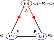
Figure 1: Color online. Resonant triad $\Delta_{1}$, see Tab. 1 below. Wave numbers of modes $m\,,\ \ell$ are shown inside ovals. Red arrows are coming from an active mode A (with frequency $\omega_{3}=\omega_{1}+\omega_{2}$) and show directions of the energy flux to the passive P-modes (with frequencies $\omega_{1}$ and $\omega_{2}$).

II Atmospheric planetary waves

II.1 Barotropic vorticity equation on a sphere

Planetary waves in the atmosphere pose a rich and complicated problem which is influenced by the earth topography, the vertical temperature profiles (varying between land and ocean), global winds etc. We do not attempt here to take into account all this richness. The essence of the interesting dynamics can be gleaned from simplified models. A very simplified model of atmospheric planetary waves (discussed, e.g. by Silberman 54sil ) is provided by the barotropic vorticity equation on a rotating sphere for the dimensionless stream function $\psi(\theta,\varphi,t)$. The variables $t,\theta$ and $\varphi$ are the time, the latitude ($-\pi/2\leq\theta\leq\pi/2$) and longitude ($0\leq\varphi\leq 2\pi$) on the sphere. The equation reads 54sil :

$$\Delta\frac{\partial\psi}{\partial t} = \frac{1}{\sin\theta}\Big{(}\frac{\partial\psi}{\partial\varphi}\frac{\partial}{\partial\theta}-\frac{\partial\psi}{\partial\theta}\,\frac{\partial}{\partial\varphi}\Big{)}\Big{(}2\,\Omega\cos\theta+\Delta\psi\Big{)}\,,$$

$$\Delta = \frac{1}{\sin\theta}\Big{[}\frac{\partial}{\partial\theta}\Big{(}\sin\theta\frac{\partial}{\partial\theta}\Big{)}+\frac{1}{\sin\theta}\frac{\partial^{2}}{\partial\varphi^{2}}\Big{]}\,,$$ (5)

where $\Delta$ is the angular part of the spherical Laplacian operator. The stream-function gives rise to the velocity ${\bm{v}}=\Omega\,R\,[\bf z\times\bm{\nabla}\psi]$, where $\Omega$ and $R$ are the angular velocity and radius of the Earth and $\bf z$ is the vertical unit vector.

Equation (II.1) conserves the energy $E$ and the enstrophy $H$, which are defined by:

$$E = \frac{1}{2}\int\limits_{0}^{2\pi}d\varphi\int\limits_{0}^{\pi}|\nabla\psi|^{2}\sin\theta d\theta\,,$$ (6a)

$$H = \frac{1}{2}\int\limits_{0}^{2\pi}d\varphi\int\limits_{0}^{\pi}|\Delta\psi|^{2}\sin\theta d\theta\ .$$ (6b)

II.2 Projection on the spherical basis

The eigenfunctions of the linear part of Eq. (II.1) are

$$\Psi_{j}\equiv\Psi_{\ell_{j}}^{m_{j}}(\theta,\varphi,t)=Y_{j}(\theta,\varphi)\,\exp(\,i\,\omega_{j}\,t)\,,$$ (7a)

where the frequencies of planetary waves are:

$$\omega_{j}\equiv\omega(\ell_{j},m_{j})=-{2\,m_{j}\Omega}\Big{/}{\ell_{j}(\ell_{j}+1)}\ .$$ (7b)

From now on we use the shorthand notation $$j=(\ell_{j},m_{j}) \ell_{j},m_{j} Y_{\ell_{j}}^{m_{j}}(\theta,\varphi)$$ for the eigen-numbers of the spherical harmonic

$$Y_{j}\equiv Y_{\ell_{j}}^{m_{j}}(\theta,\varphi)=P_{\ell_{j}}^{m_{j}}(\cos\theta)\,\exp(i\,m_{j}\,\varphi)\,,$$ (7c)

with the associated Legendre polynomials $$P_{j}\equiv P_{\ell_{j}}^{m_{j}}(\cos\theta)$$, normalized as follows:

$$\int_{0}^{\pi}P_{\ell}^{m}P_{\ell^{\prime}}^{m}\sin\theta d\theta=\delta(\ell,\ell^{\prime})\ ,\quad P_{\ell}^{-m}=P_{\ell}^{m}\ .$$ (7d)

Here $$\delta(\ell,\ell^{\prime}) \ell=\ell^{\prime} m (\ell-m) \ell,m m \ell 40\,000 \ell\lesssim 1000$$ is the Kronecker symbol (1 for and zero otherwise). The integer indices and are the longitudinal and latitudinal wave-numbers of the -mode; they count the number of zeros of the spherical function along the longitudinal and the latitudinal directions. Below we refer to the range of and as the “spectral domain”. For the approximation of two-dimensional atmosphere to hold, the wave-length is supposed to be much smaller than the atmosphere’s hight. If we estimate the wave-length as the distance between the appropriate zeroes of spherical function, the length of the equator at about km and the height of the atmosphere at about 40 km, we understand that the approximation of a two-dimensional atmosphere holds up to .

Expanding the function $\psi(\theta,\varphi,t)$ in the basis (7a) we get

$$\psi(\theta,\varphi,t)=\sum_{j}A_{j}\Psi_{j}\ .$$ (7e)

Substituting in Eq. (II.1) one obtains the governing equations for the “slow” amplitudes $A_{j}\equiv A_{\ell_{j}}^{m_{j}}(t)$ of the planetary waves:

$$\frac{dA_{j}}{dt} = \frac{i}{2\,N_{j}}\sum_{r,s}N_{r,s}\,Z_{j|r,s}\,A_{r}\,A_{s}$$

$$\times\exp[i(\omega_{r}+\omega_{s}-\omega_{j})t]\delta(m_{j},m_{r}+m_{s})\,,$$

$$N_{j} \equiv \ell_{j}(\ell_{j}+1)\,,\quad N_{r,s}\equiv N_{r}-N_{s}\,,$$ (8b)

where the three-wave interaction coefficients are

$$Z_{j|r,s}\equiv Z_{\ell_{j}}^{m_{j}}|_{\ell_{r},\,~{}\ell_{s}}^{m_{r},m_{s}}=\int\limits_{0}^{\pi}{\mathcal{Z}}_{j|r,s}(\theta)\,d\theta\,,$$ (9a)

with the “interaction integrand”

$${\mathcal{Z}}_{j|r,s}(\theta)=P_{\ell_{j}}^{m_{j}}\Big{[}m_{r}P_{\ell_{r}}^{m_{r}}\frac{dP_{\ell_{s}}^{m_{s}}}{d\theta}-m_{s}P_{\ell_{s}}^{m_{s}}\frac{dP_{\ell_{r}}^{m_{r}}}{d\theta}\Big{]}\ .~{}~{}$$ (9b)

We note that Eq. (8) is an exact consequence of the barotropic vorticity equation, without any assumption about the existence of a small parameter. Among the interactions appearing in this equations there are many non-resonant ones, in which the exponent $\exp[i(\omega_{r}+\omega_{s}-\omega_{j})t]$ is not unity. All these interactions can be removed by a change of variables, which however will result in new nonlinear terms (higher than quadratic), see e.g. Sec. 1.1.4 in ZLF . Assuming that the wave amplitudes are small enough, all these can be disregarded, bringing the final equations back to the same form as in Eq. (8), but including only resonant triads for which $\exp[i(\omega_{r}+\omega_{s}-\omega_{j})t]=1$.

II.3 Necessary conditions for non-vanishing interaction

The first necessary condition that guarantees finite interaction amplitudes follows from the axial symmetry of the problem and is reflected in the Kronecker symbol in Eq. (8):

$$m_{j}=m_{r}+m_{s}\ .$$ (10a)

Second, the spherical symmetry of the nonlinear term in Eq. (II.1) leads to the conservation of the square of the total angular momentum of the system. This translates to the triangle inequality for vectors $${\bm{\ell}}_{j}={\bm{\ell}}_{r}+{\bm{\ell}}_{s}$$ in each triangle with non-zero interaction amplitude:

$$|\ell_{r}-\ell_{s}|<\ell_{j}<\ell_{r}+\ell_{s}\ .$$ (10b)

Third, the explicit form of Eq. (9a) requires that

$$\ell_{j}+\ell_{r}+\ell_{s}\quad\mbox{ is odd.}$$ (10c)

Otherwise integrand (9b) is odd function of $\cos\theta$ and integral (9a) is zero.

It can be shown by integrating Eq. (9) by parts that whenever Eq. (10a) is fulfilled the three interaction coefficients satisfy:

$$Z_{\ell_{j}}^{m_{j}}|_{\ell_{r},\,~{}\ell_{s}}^{m_{r},m_{s}}=Z_{\ell_{s}}^{m_{s}}|_{\ \ \ell_{r},~{}\ell_{j}}^{-m_{r},m_{j}}=Z_{\ell_{r}}^{m_{r}}|_{\ \ell_{j},\ \ell_{s}}^{m_{j},-m_{s}}\ .$$ (11)

From this follows that the interaction coefficients $Z_{\dots}$ satisfy two Jacoby identities

$$Z_{j|r,s}+Z_{r|s,j}+Z_{s|j,r} = 0\,,$$ (12)

$$N_{j}Z_{j|r,s}+N_{r}Z_{r|s,j}+N_{s}Z_{s|j,r} = 0\ .$$

As a result, Eqs. (8) have two integrals of motion

$$E = \frac{1}{2}\sum_{j}N_{j}|A_{j}|^{2}\,,$$ (13a)

$$H = \frac{1}{2}\sum_{j}N_{j}^{2}|A_{j}|^{2}\,,$$ (13b)

which are nothing else but the energy (6a) and enstrophy (6b), presented in the basis (7).

${\mathcal{A}}$	${\mathcal{B}}$	${\mathcal{C}}$
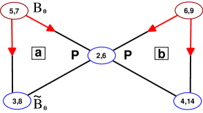
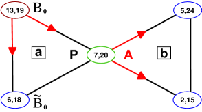
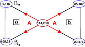
PP-butterfly	PA-butterfly	AA-butterfly

Figure 2: Color online. Examples of isolated butterflies. All the notations are as in Fig. 1. In particular: red arrows are coming from the active modes A and show directions of the energy flux to the passive P-modes. The letters “a” and “b” in square boxes denote triads and will be used as subscripts in the corresponding evolution equations for amplitudes and for integrals of motion. In studies of free evolution in Sec. V the initial energy is concentrated in the “leading” $a$-triad in “individual” modes with amplitudes $B_{0}$ and $\widetilde{B}_{0}$ and then goes to the “driven” $b$-triad.

III Small clusters of resonant triads

In this Section we formulate equations of motion and motion invariants of small clusters of resonant triads, study their topology and other properties, that affect on the dynamics of finite-dimensional wave turbulence. Brief analysis of these questions was given in LABEL:KL-08.

III.1 Active and passive modes in a resonant triad

In this paper we refer to a “resonant triad” whenever we have three modes $(j,r,s)$ whose frequencies satisfy the triad resonance condition $\omega_{j}=\omega_{r}+\omega_{s}$. Accordingly, the equations for the slow amplitudes of modes in resonant triads are written, (after relabeling according to $r\to 1$, $s\to 2$ and $j\to 3$) as follows:

$$N_{1}\frac{dA_{1}}{dt} = iN_{3,2}ZA_{2}^{*}A_{3}\,,\quad Z\equiv Z_{3|1,2}\,,$$

$$N_{2}\frac{dA_{2}}{dt} = iN_{1,3}ZA_{1}^{*}A_{3}\,,$$ (14)

$$N_{3}\frac{dA_{3}^{*}}{dt} = iN_{2,1}ZA_{1}^{*}A_{2}^{*}\ .$$

In this case the conservation laws (13) take the form:

$$E = \frac{1}{2}\left(N_{1}|A_{1}|^{2}+N_{2}|A_{2}|^{2}+N_{3}|A_{3}|^{2}\right)\,,$$ (15a)

$$H = \frac{1}{2}\left(N_{1}^{2}|A_{1}|^{2}+N_{2}^{2}|A_{2}|^{2}+N_{3}^{2}|A_{3}|^{2}\right)\ .$$ (15b)

Taking for concreteness an example for which

$$\ell_{1}>\ell_{3}>\ell_{2}\ ,$$ (16)

we make in Eqs. (14) a linear change of variables $B_{i}=\alpha_{i}A_{i}$ such that

$$\alpha_{1} = -i\sqrt{N_{1,2}N_{1,3}}/\sqrt{N_{2}N_{3}}\,,$$

$$\alpha_{2} = i\sqrt{N_{1,2}N_{3,2}}/\sqrt{N_{1}N_{3}}\,,$$ (17)

$$\alpha_{3} = i\sqrt{N_{1,3}N_{3,2}}/\sqrt{N_{1}N_{2}}\ .$$

This results in equations with real coefficients that involve only one interaction amplitude $Z$:

$$\frac{dB_{1}}{dt} = ZB_{2}^{*}B_{3}\,,$$

$$\frac{dB_{2}}{dt} = ZB_{1}^{*}B_{3}\,,$$ (18)

$$\frac{dB_{3}}{dt} = -ZB_{1}B_{2}\ .$$

This is a dynamical system corresponding to the simplest possible resonant cluster. Equations (18) are symmetric with respect to replacing two low-frequency modes $1\Leftrightarrow 2$. The mode with highest frequency (which in this paper will be always denoted by subscript “ ${}_{3}~{}$”) is special. When Eq. (16) does not hold one can find a similar change of variable for any relations between the magnitudes of the three indices $\ell_{j}$.

The system (18) has two independent conservation laws (known as Manley-Rowe integrals)

$$\begin{cases}I_{23}=|B_{2}|^{2}+|B_{3}|^{2}=(E\,N_{1}-H){N_{23}}/{N_{1}N_{2}N_{3}}\,,\\ I_{13}=|B_{1}|^{2}+|B_{3}|^{2}=(E\,N_{2}-H){N_{13}}/{N_{1}N_{2}N_{3}}\,,\\ I_{12}=I_{13}-I_{23}=|B_{1}|^{2}-|B_{2}|^{2}\,,\end{cases}$$ (19)

which are linear combinations of the energy $E$ and enstrophy $H$ defined by Eqs. (15).

Obviously, Eq. (18) can be written in the Hamiltonian form:

$$i\,\frac{dB_{j}}{dt}=\frac{dH_{\text{int}}}{dB_{j}^{*}}\,,$$ (20a)

with the interaction Hamiltonian

$$H_{\text{int}}=iZ(B_{1}B_{2}B_{3}^{*}-B_{1}^{*}B_{2}^{*}B_{3})\,,$$ (20b)

which is an additional integral of motion. In terms of old variables $$A_{j}$$

$$H_{\text{int}}=iZ\,\frac{N_{1,2}N_{1,3}N_{3,2}}{N_{1}N_{2}N_{3}}(A_{1}A_{2}A_{3}^{*}-A_{1}^{*}A_{2}^{*}A_{3})\ .$$ (20c)

By direct calculation it is easy to check that Eq. (20c) is an integral of motion of the dynamical system Eq. (14).

On the face of it Eqs. (18) involves six dynamical variables: i.e. $B$’s and their complex conjugates. In fact, using the standard representation of the complex amplitudes $B_{j}$ in terms of real amplitudes $C_{j}$ and phases $\theta_{j}$:

$$B_{j}=C_{j}\exp(i\theta_{j})\,,$$ (21a)

one recognizes that the right-hand-side (RHS) of Eq. (18) depends only on a single combination of phases in the triad which affects the dynamics. We refer to this combination as the triad phase:

$$\varphi\equiv\theta_{1}+\theta_{2}-\theta_{3}\ .$$ (21b)

The triad phase appears in Eq. (20b) as follows:

$$H_{\text{int}}=-2\,Z|B_{1}B_{2}B_{3}|\sin\varphi\ .$$ (22)

Thus we have a four dimensional phase space with three integrals of motion, resulting in a simple periodic trajectory for almost all conditions. For more details see  KL-07 . Nevertheless even this simple dynamics offers the first opportunity to discuss the energy flow within a cluster of interacting modes.

To this aim we discuss the evolution of the triad of amplitudes with special initial conditions, when only one mode is appreciably excited at zero time. If $B_{1}(t=0)\gg B_{2}(t=0)$ and $B_{1}(t=0)\gg B_{3}(t=0),$ then $I_{23}(t=0)\ll I_{13}(t=0)$. The integrals of motion are independent of time, therefore $I_{13}\gg I_{23}$ at all later times, and hence $|B_{1}(t)|^{2}\gg|B_{2}(t)|^{2}$. Moreover, $|B_{1}(t)|^{2}\gg|B_{3}(t)|^{2}$ at all times. Indeed, the assumption $|B_{1}(t)|^{2}\lesssim|B_{3}(t)|^{2}$ yields $I_{13}\simeq I_{23}$, which is not tenable. This means that the $\omega_{1}$-mode, being the only essentially exited one at $t=0$ cannot redistribute its energy to the other two modes in the triad. The same is true for the $\omega_{2}$-mode. For this reason we refer to the lower frequency modes with frequencies $\omega_{1}<\omega_{3}$ and $\omega_{2}<\omega_{3}$ “passive modes”, or P-modes.

On the other hand, the conservation laws (19) cannot restrict the growing of P-modes from initial conditions when only $\omega_{3}$-mode is appreciably excited. In this case the P-mode amplitudes will grow exponentially Has-67 : $|B_{1}(t)|\,,\ |B_{2}(t)|\propto\exp[\,|ZB_{3}(t=0)|t]$ until all the modes will have comparable magnitudes of their amplitudes. Therefore we refer to the $\omega_{3}$-mode as an “active mode”, or A-mode. An A-mode, being initially excited, is capable of shearing its energy with two P-modes within the triad.

III.2 Double-triad clusters: Butterflies

An arbitrary cluster in our wave system is a set of connected triads. Examples of the simplest clusters, consisting of two triads connected via one common mode are shown in Fig. 2. They will be referred to as butterflies. Note that in principle one can have two triads connected by two modes, but such a cluster does not satisfy all the conditions stated above.

The dynamics of a cluster depends on the type of the mode which is common for the neighboring triads. Correspondingly we can distinguish three types of butterflies: PP-, AP- and AA-butterflies, In this Section we consider the equations of motion, the invariants and the restrictions on dynamical behavior, that follow from the existence of invariants for relatively small clusters consisting of two triads. In the following Secs. we consider these questions for clusters consisting of three and six triads.

Butterflies, as shown in Fig. 2, consist of two triads $\ a\$ and $\ b,\$ with wave amplitudes $\ B_{j|a},\ B_{j|b},\$ $j=1,2,3$, connected via one common mode. For PP-butterfly the common mode is passive in both triads, say

$$\ B_{1|a}=B_{1|b}\qquad\mbox{PP-butterfly}\,;$$ (23a)

for an PA-butterfly the common mode is passive in $$a b$$-triad and active in the second, -triad:

$$\ B_{1|a}=B_{3|b}\qquad\mbox{PA-butterfly}\,;$$ (23b)

while for an AA-butterfly the common mode is active in both triads:

$$\ B_{3|a}=B_{3|b}\qquad\mbox{AA-butterfly}\ .$$ (23c)

The equations of motion for these systems follow from the Eqs. (8) under the condition of small nonlinearity and from the resonance conditions in both triads:

$$\omega_{1|a}+\omega_{2|a}=\omega_{3|a}\,,\quad\omega_{1|b}+\omega_{2|b}=\omega_{3|b}\,,$$ (24)

with the obvious requirement that the frequencies of the common modes are the same. After a change of variables similar to Eqs. (17) and elimination of one common mode, the resulting equations for PP-butterfly ($B_{1|a}=B_{1|b}$) are:

$$\begin{cases}\dot{B}_{1|a}=Z_{a}B_{2|a}^{*}B_{3|a}+Z_{b}B_{2|b}^{*}B_{3|b},\,,\\ \dot{B}_{2|a}=Z_{a}B_{1|a}^{*}B_{3|a}\,,\quad\dot{B}_{2|b}=Z_{b}B_{1|a}^{*}B_{3|b}\,,\\ \dot{B}_{3|a}=-Z_{a}B_{1|a}B_{2|a}\,,\ \dot{B}_{3|b}=-Z_{b}B_{1|a}B_{2|b}\ .\\ \end{cases}$$ (25a)

For PA-butterfly (with $$B_{1|a}=B_{3|b}$$) they are

$$\begin{cases}\dot{B}_{1|b}=Z_{b}B_{2|b}^{*}B_{3|b}\,,\quad\dot{B}_{3|a}=-Z_{a}B_{3|b}B_{2|a}\,,\\ \dot{B}_{2|b}=Z_{b}B_{1|b}^{*}B_{3|b}\,,\quad\dot{B}_{2|a}=Z_{a}B_{3|b}^{*}B_{3|a}\,,\\ \dot{B}_{3|b}=-Z_{b}B_{1|b}B_{2|b}+Z_{a}B_{2|a}^{*}B_{3|a}\,,\end{cases}$$ (25b)

and for AA-butterfly (with $$B_{3|a}=B_{3|b}$$):

$$\begin{cases}\dot{B}_{1|a}=Z_{a}B_{2|a}^{*}B_{3|a}\,,\ \dot{B}_{1|b}=+Z_{b}B_{2|b}^{*}B_{3|a}\,,\\ \dot{B}_{2|a}=Z_{a}B_{1|a}^{*}B_{3|a}\,,\quad\dot{B}_{2|b}=Z_{b}B_{1|b}^{*}B_{3|a}\,,\\ \dot{B}_{3|a}=-Z_{a}B_{1|a}B_{2|a}-Z_{b}B_{1|b}B_{2|b}\ .\\ \end{cases}$$ (25c)

All these equations can be obtained from the canonical equations of motion (20a) using the Hamiltonian

$$H_{\rm int}=2{\rm Im}\left\{Z_{a}B_{1|a}^{*}B_{2|a}^{*}B_{3|a}+Z_{b}B_{1|b}^{*}B_{2|b}^{*}B_{3|b}\right\}\ ,$$ (26)

in which the conditions (23) have to be fulfilled for each particular butterfly.

${\mathcal{A}}$	${\mathcal{B}}$
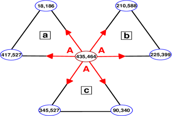
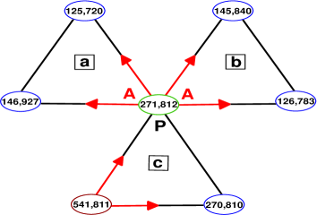
One of tree AAA-stars	One of five AAP-stars
${\mathcal{C}}$	${\mathcal{D}}$
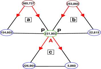
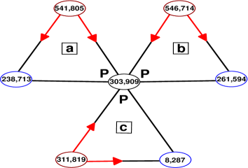
One of six APP-stars	One of eleven PPP-stars

Figure 3: Color online. Examples of isolated triple stars in the spectral domain $m\leq\ell\leq 1000$. The letters “a”, “b” and “c” in square boxes denote triads and will be used as subscripts in the corresponding evolution equations for amplitudes and for integrals of motion. All other notations as in Fig. 1 and 2.

${\mathcal{A}}$	${\mathcal{B}}$	${\mathcal{C}}$
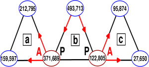
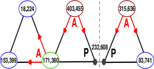
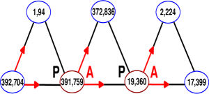
AP-PA triple chain cluster	One of five AP-PP chains	One of six PA-PA chains
${\mathcal{D}}$	${\mathcal{E}}$	${\mathcal{F}}$
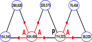
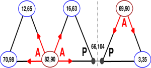
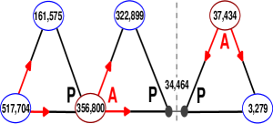
One of six AA-PA chains	One of fourteen AA-PP chains	One of sixteen PA-PP chains
${\mathcal{G}}$	${\mathcal{H}}$	${\mathcal{I}}$
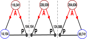
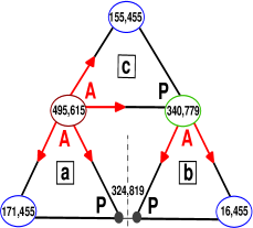
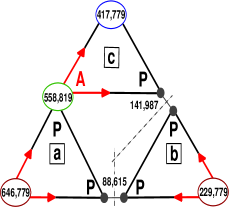
one of eighteen PP-PP chains	One of two AA-PA-PP triangles	One of two PA-PP-PP triangles

Figure 4: Color online. In the spectral domain $m\leq\ell\leq 1000$ there are 66 isolated triple-chain clusters of seven types (examples are shown in panels ${\mathcal{A}}-{\mathcal{F}}$) and four triangle clusters with (AA-PA-PP)- and (PA-PP-PP)-connections (examples are shown in panels ${\mathcal{H}}\,,{\mathcal{I}}$)). Common PP-modes are split, denoting difficulty in the energy exchange between corresponding triads. Dashed lines separate PP-irreducible sub-clusters, discussed in Sec. IV.2.

In addition to the Hamiltonian (26) we have three more invariants of the Manley-Rowe type for each butterfly. For the PP-, PA- and AA-butterflies they respectively are

$$I_{2,3|a} = |B_{2|a}|^{2}+|B_{3|a}|^{2}\,,\quad I_{2,3|b}=|B_{2|b}|^{2}+|B_{3|b}|^{2}\,,$$

$$I_{|a,b} = |B_{1|a}|^{2}+|B_{3|a}|^{2}+|B_{3|b}|^{2}\ ,\ {\rm PP;}$$ (27a)

$$I_{1,2|b} = |B_{1|b}|^{2}-|B_{2|b}|^{2}\,,\quad I_{2,3|a}=|B_{2|a}|^{2}+|B_{3|a}|^{2}\,,$$

$$I_{|a,b} = |B_{1|b}|^{2}+|B_{3|b}|^{2}+|B_{3|a}|^{2}\ ,\ {\rm PA;}$$ (27b)

$$I_{1,2|a} = |B_{1|a}|^{2}-|B_{2|a}|^{2}\,,\quad I_{1,2|b}=|B_{1|b}|^{2}-|B_{2|b}|^{2}\,,$$

$$I_{|a,b} = |B_{1|a}|^{2}+|B_{1|b}|^{2}+|B_{3|a}|^{2}\ ,\quad{\rm AA.}$$ (27c)

The first two invariants for the PP butterfly, $I_{2,3|a}$ and $I_{2,3|b}$, do not involve the common mode $B_{1|a}=B_{1|b}$, and are similar to the invariant $I_{23}$, Eq. (19), for an isolated triad. We can make the following observation: If at $t=0$ the amplitudes in one triad exceed substantially the two remaining amplitudes of the butterfly, that is $|B_{1|a}|,|B_{2|a}|,|B_{3|a}|\gg|B_{2|b}|,|B_{3|b}|$, this relation persists. In other words, in PP-butterfly when any of the two triads, $a$ or $b$, has initially very small amplitudes, it is unable to absorb the energy from the second triad during the nonlinear evolution.

The invariants $I_{1,2|b}$ and $I_{2,3|a}$ for the PA butterfly do not involve the common mode $\ B_{3|b}=B_{1|a}$ ; they are similar to the corresponding integrals $I_{12}$ and $I_{23}$, Eqs. (19), for an isolated triad. If at $t=0$ the $b$-triad is excited much more than the $a$-triad (and thus $\ I_{1,2|b}\gg I_{2,3|a}$) the smallness of the positively defined invariant $I_{2,3|a}$ prevents the $a$-triad from absorbing energy from $b$-triad during the time evolution. The situation is different when the $a$-triad is initially excited and $\ I_{2,3|a}\gg I_{1,2|b}$. In this case the initial energy of $a$-triad can be easily shared with $b$-triad. The smallness of $I_{1,2|b}$ only requires that during evolution $|B_{1|b}|\approx|B_{2|b}|$. Under this type of the initial conditions we will call the $a$-triad “leading” triad, while the $b$-triad will be referred to as ”driven” triad.

Finally, the invariants for the AA butterfly, $I_{1,2|a}$ and $I_{1,2|b}$, do not involve the common mode $\ B_{3|a}=B_{1|b}$ and are similar to $I_{12}$, Eqs. (19), for isolated triad. Simple analysis of these integrals of motion shows that energy, initially held in one of the triads will be shared between both triads dynamically.

The conclusion that we can draw from these examples is general: any triad which is connected to any given cluster of any size whatsoever where the connection occurs via its passive mode cannot absorb the energy from the cluster, if initially the triad is not excited. In contrast, a triad connected to a cluster of any given size via an active mode can freely adsorb energy from the cluster during the nonlinear evolution.

III.3 Triple-triad clusters: stars, chains and triangles

Triple triad clusters consist of three triads, denoted as $a$-, $b$- and $c$-triads with the mode amplitudes denoted as $B_{j|a}$, $B_{j|b}$, $B_{j|c}$, $j=1,2,3$. There are three topologically different types of triple-triad clusters: with one common mode – stars, shown in Figs. 3; with two common modes – chains, and with three common modes – triangles, these clusters are shown in Fig. 4. Having in mind different types of common modes one distinguishes 13 types of triple-triad clusters, including four stars (AAA-, AAP-, APP-, PPP-stars, Fig. 3), 7 types of 3-chain-, and two types of triangle-clusters, in Fig. 4. All motion equations can be written in the canonical form (20a) with the Hamiltonian

$$H_{\rm int} = 2{\rm Im}\Big{\{}Z_{a}B_{1|a}^{*}B_{2|a}^{*}B_{3|a}+Z_{b}B_{1|b}^{*}B_{2|b}^{*}B_{3|b}$$ (28)

$$~{}~{}~{}~{}~{}~{}+Z_{c}B_{1|c}^{*}B_{2|c}^{*}B_{3|c}\Big{\}}\ ,$$

in which one has to equate amplitudes of common modes.

Stars

have one common mode in three triads. For example, taking $B_{3|a}=B_{3|b}=B_{3|c}$ in Eq. (28) one gets from Eq. (20) equations of motion for AAA-stars:

$$\begin{cases}\dot{B}_{1|a}=Z_{a}B_{2|a}B_{3|a}\,,\quad\dot{B}_{2|a}=Z_{a}B_{1|a}B_{3|a}\,,\\ \dot{B}_{1|b}=Z_{b}B_{2|b}B_{3|a}\,,\quad~{}\dot{B}_{2|b}=Z_{a}B_{1|b}B_{3|a}\,,\\ \dot{B}_{1|c}=Z_{c}B_{2|c}B_{3|a}\,,\quad~{}\,\dot{B}_{2|c}=Z_{c}B_{1|c}B_{3|a}\,,\\ \dot{B}_{3|a}=-Z_{a}B_{1|a}B_{2|a}-Z_{b}B_{1|b}B_{2|b}-Z_{c}B_{1|c}B_{2|c}\ .\end{cases}$$ (29a)

Taking $$B_{3|a}=B_{3|b}=B_{1|c}$$ one gets for AAP-stars:

$$\begin{cases}\dot{B}_{1|a}=Z_{a}B_{2|a}B_{3|a}\,,\quad\,\,\dot{B}_{2|a}=Z_{a}B_{1|a}B_{3|a}\,,\\ \dot{B}_{1|b}=Z_{b}B_{2|b}B_{3|a}\,,\quad~{}\,\,\dot{B}_{2|b}=Z_{a}B_{1|b}B_{3|a}\,,\\ \dot{B}_{3|c}=-Z_{c}B_{3|a}B_{2|c}\,,\quad\dot{B}_{2|c}=Z_{c}B_{3|a}B_{3|c}\,,\\ \dot{B}_{3|a}=-Z_{a}B_{1|a}B_{2|a}-Z_{b}B_{1|b}B_{2|b}+Z_{c}B_{2|c}B_{3|c}\ .\end{cases}$$ (29b)

Similarly one gets motion equations for:

$$\mbox{PPA-star:}\qquad B_{1|a}=B_{1|b}=B_{3|c}\,,$$

$$\begin{cases}\dot{B}_{3|a}=-Z_{a}B_{1|a}B_{2|a}\,,\quad\dot{B}_{2|a}=Z_{a}B_{1|a}B_{3|a}\,,\\ \dot{B}_{3|b}=-Z_{b}B_{1|a}B_{2|b}\,,\quad\ \dot{B}_{2|b}=Z_{a}B_{1|a}B_{3|b}\,,\\ \dot{B}_{1|c}=Z_{c}B_{2|c}^{*}B_{1|a}\,,\qquad\dot{B}_{2|c}=Z_{c}B_{1|a}B_{1|c}\,,\\ \dot{B}_{1|a}=Z_{a}B_{2|a}^{*}B_{3|a}+Z_{b}B_{2|b}^{*}B_{3|b}-Z_{c}B_{1|c}B_{2|c}\ .\end{cases}$$ (29c)

$$\mbox{PPP-star:}\qquad B_{1|a}=B_{1|b}=B_{1|c}\,,\,,$$

$$\begin{cases}\dot{B}_{3|a}=-Z_{a}B_{1|a}B_{2|a}\,,\quad\dot{B}_{2|a}=Z_{a}B_{1|a}B_{3|a}\,,\\ \dot{B}_{3|b}=-Z_{b}B_{1|a}B_{2|b}\,,\quad\ \dot{B}_{2|b}=Z_{a}B_{1|a}B_{3|b}\,,\\ \dot{B}_{3|c}=-Z_{c}B_{1|a}B_{2|c}\,,\quad\ \dot{B}_{2|c}=Z_{c}B_{1|a}B_{3|c}\,,\\ \dot{B}_{1|a}=Z_{a}B_{2|a}^{*}B_{3|a}+Z_{b}B_{2|b}^{*}B_{3|b}+Z_{c}B_{2|c}B_{3|c}\ .\end{cases}$$ (29d)

In addition to Hamiltonian, all triple-star clusters have four invariants of the Manley-Rowe type, three of them does not involve the common mode. For example, for

$$\begin{cases}\mbox{PPA-star: }\qquad I_{1,2|a}=|B_{1|a}|^{2}-|B_{2|a}|^{2}\,,\\ I_{2,3|b}=|B_{2|b}|^{2}+|B_{3|b}|^{2}\,,\quad I_{2,3|c}=|B_{2|c}|^{2}+|B_{3|c}|^{2}\,,\\ I_{|a,b,c}=|B_{1|a}|^{2}+|B_{3|a}|^{2}+|B_{3|b}|^{2}+|B_{3|c}|^{2}\ .\end{cases}$$ (30)

Integrals $I_{2,3|b}$ and $I_{2,3|c}$ prevent $b$- and $c$-triads (connected via the P-mode) from adopting energy of initially excited $a$-triad. In cases when $b$- and/or $c$-triad are initially exited, $a$-triad can freely share their energy via connecting A-mode.

Triple-chains

have two common modes in two triads. As we mentioned, there are 7 types of triple-chains, that differ in type of connections, see Fig. 4. Similarly to the triple-star clusters, one gets equation of motion for triple-chains from the canonical  Eq. (20a) with the Hamiltonian (28), in which one has to equate two pairs of amplitudes of common modes. For example, for PA-PA chain,

$$\mbox{PA-PA-chain:}\quad B_{1|a}=B_{3|b}\,,\quad B_{1|b}=B_{3|c}\,,$$ (31a)

$$\begin{cases}\dot{B}_{1|a}=Z_{a}B_{2|a}^{*}B_{3|a}-Z_{b}B_{1|b}B_{2|b}\,,\\ \dot{B}_{2|a}=Z_{a}B_{1|a}^{*}B_{3|a}\,,\quad\dot{B}_{3|a}=-Z_{a}B_{1|a}B_{2|a}\,,\\ \dot{B}_{2|b}=Z_{b}B_{1|b}^{*}B_{3|b}\,,\\ \dot{B}_{1|b}=Z_{b}B_{2|b}^{*}B_{3|b}-Z_{a}B_{1|c}B_{2|c}\,,\\ \dot{B}_{1|c}=Z_{c}B_{2|c}^{*}B_{1|b}\,,\quad\dot{B}_{2|c}=Z_{c}B_{1|c}^{*}B_{1|b}\ .\end{cases}$$ (31b)

Again, besides Hamiltonian, all triple-chain clusters have four invariants of the Manley-Rowe type, two of them do not involve the common mode. In particular, PA-PA chain, governed by Eq. (31a) has the following invariants:

$$\begin{cases}\mbox{PA-PA chain: }\qquad I_{|a,b}=|B_{1|a}|^{2}-|B_{2|a}|^{2}+|B_{2|b}|^{2}\,,\\ ~{}\,I_{|b,c}=|B_{1|b}|^{2}-|B_{2|b}|^{2}+|B_{2|c}|^{2}\,,\\ I_{2,3|a}=|B_{2|a}|^{2}+|B_{3|a}|^{2}\,,\quad I_{1,2|c}=|B_{1|c}|^{2}-|B_{2|c}|^{2}\ .\end{cases}$$ (31c)

Triple-triangles

have three common modes in three triads, see Fig. 4$\,{\mathcal{H}}$ and ${\mathcal{I}}$. Correspondingly, equations of motion for AA-PA-PP and PA-PP-PP triangles one gets from the canonical  Eq. (20a) with the Hamiltonian (28), in which one has to equate three pairs of amplitudes of common modes. In particular, for AA-PA-PP triangle one has:

$$B_{1|a}=B_{1|b}\,,\ B_{3|a}=B_{3|c}\,,\ B_{3|b}=B_{1|c}\,,$$ (32a)

$$\begin{cases}\dot{B}_{1|a}=Z_{a}B_{2|a}^{*}B_{3|a}+Z_{b}B_{2|b}^{*}B_{3|b}\,,\\ \dot{B}_{2|a}=Z_{a}B_{1|a}^{*}B_{3|a}\,,\\ \dot{B}_{3|a}=-Z_{a}B_{1|a}B_{2|a}-Z_{c}B_{2|c}B_{3|b}\,,\\ \dot{B}_{2|b}=Z_{b}B_{1|a}^{*}B_{3|b}\,,\\ \dot{B}_{3|b}=-Z_{b}B_{1|a}B_{2|b}+Z_{c}B_{2|c}^{*}B_{3|a}\,,\\ \dot{B}_{2|c}=Z_{c}B_{3|b}^{*}B_{3|a}\ .\end{cases}$$ (32b)

Triangle clusters have three Manley-Rowe invariants. In particular, AA-PA-PP triangle, governed by Eq. (32b) has the following invariants:

$$\begin{cases}\mbox{AA-PA-PP triangle: }\qquad I_{|a,b}=|B_{2|b}|^{2}-|B_{1|a}|^{2}\,,\\ I_{|a,c}=|B_{2|a}|^{2}+|B_{3|a}|^{2}+|B_{2|c}|^{2}\,,\\ I_{|b,c}=|B_{2|b}|^{2}-|B_{3|b}|^{2}-|B_{2|c}|^{2}\ .\end{cases}$$ (32c)

Notice, that triple-stars and triple-chains have 10 real variables (seven amplitudes and three triad phases) and five invariants (Hamiltonian and four Manley-Rowes’), while triple-triangles have only 9 real variables (six amplitudes and three triad phases) and four invariants (Hamiltonian and three Manley-Rowes’). Therefore, all triple-triad clusters have five-dimensional effective phase space. Recall, that butterflies have three-dimensional phase space. Moreover, one can prove that any $n$-triad cluster has $(2n-1)$-dimensional effective phase space.

III.4 Caterpillar: 6-triad cluster

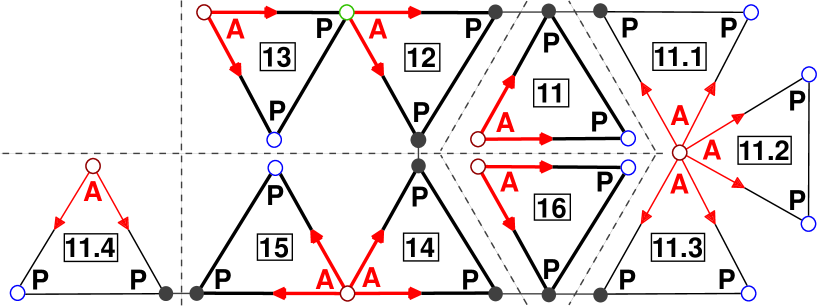
Figure 5: Color online. Triads belonging to caterpillar are drawn by bold lines. New, connected to them triads, appearing in spectral domain $m,\ell\leq 1000$ are drawn by thin lines. The PP-reduction of the extended caterpillar to three triads ($\Delta_{11}$, $\Delta_{16}$ and $\Delta_{11.4}$, according to Tab. 1), PA-butterfly $\bowtie_{12,13}$, AA–butterfly $\bowtie_{14,15}$, and AAA-star is shown by dashed lines. The rest of notations as in Figs. 1 and 4.

The largest cluster found in the domain $\ell<21$ consists of six resonant triads $\Delta_{11}\dots\Delta_{16}$ with three PP-, one AP- and one AA-connection, see Fig. 5. The equation of motion for this cluster, (called “caterpillar”) can be obtained from Hamiltonian, similar to Eq. (28), but consisting of six terms:

$$H_{\text{cat}}=2\,\mbox{Im}\sum_{n=11}^{16}Z_{n}B_{1|n}^{*}B_{2|n}^{*}B_{3|n}\,,$$ (33a)

in which we have to equate amplitudes of common modes:

$$\begin{cases}B_{1|11}=B_{1|12}\,,\quad B_{3|12}=B_{1|13}\,,\quad B_{2|12}=B_{1|14}\,,\\ B_{3|14}=B_{3|15}\,,\quad B_{1|14}=B_{1|16}\ .\end{cases}$$ (33b)

Due to these five connections one has only $$3\times 6-5=13$$ complex equations for remaining amplitudes:

$$\begin{cases}\dot{B}_{1|11}=Z_{11}B_{2|11}^{*}B_{3|11}+Z_{12}B_{2|12}^{*}B_{3|12}\,,\\ \dot{B}_{2|11}=Z_{11}B_{1|11}^{*}B_{3|11}\,,\quad\dot{B}_{3|11}=-Z_{11}B_{1|11}B_{2|11}\,,\\ \dot{B}_{2|12}=Z_{12}B_{1|11}^{*}B_{3|12}+Z_{14}B_{1|14}^{*}B_{3|14}\,,\\ \dot{B}_{3|12}=-Z_{12}B_{1|12}B_{2|12}+Z_{13}B_{2|13}^{*}B_{3|13}\\ \dot{B}_{1|14}=Z_{14}B_{2|12}^{*}B_{3|14}+Z_{16}B_{2|16}^{*}B_{3|16}\,,\\ \dot{B}_{3|14}=Z_{14}B_{2|12}^{*}B_{1|14}+Z_{16}B_{2|16}^{*}B_{3|16}\,,\\ \dot{B}_{1|15}=Z_{15}B_{2|15}^{*}B_{3|14}\,,\quad\dot{B}_{2|15}=Z_{15}B_{1|15}^{*}B_{3|14}\,,\\ \dot{B}_{2|16}=Z_{16}B_{1|14}^{*}B_{3|16}\,,\quad\dot{B}_{3|16}=-Z_{16}B_{1|14}B_{2|16}\ .\end{cases}$$ (33c)

Caterpillar has six Manley-Rowe invariants:

$$\begin{cases}I_{2,3|11}=|B_{2|11}|^{2}+|B_{3|11}|^{2}\,,\\ I_{2,3|13}=|B_{2|13}|^{2}+|B_{3|13}|^{2}\,,\\ I_{1,2|15}=|B_{1|15}|^{2}-|B_{2|15}|^{2}\,,\\ I_{2,3|16}=|B_{2|16}|^{2}+|B_{3|16}|^{2}\,,\\ I_{|11,12,13}=|B_{1|11}|^{2}+|B_{3|11}|^{2}+|B_{3|12}|^{2}+|B_{3|13}|^{2}\,,\\ I_{|14,15,16}=|B_{1|14}|^{2}+|B_{1|15}|^{2}+|B_{3|15}|^{2}+|B_{3|16}|^{2}\ .\end{cases}$$ (33d)

Clust.	$N_{1}$	Modes $[m,\ell]$	$N_{2}$	Connecting triads
$\Delta_{1}$	$1$	[4,12] [5,14] [9,13]	$-$	$-$
$\Delta_{2}$	$2$	[3,14] [1,20] [4,15]	2.1	[4,15] [10,24] [14,20]
			2.2	[1,20] [14,29] [15,28]
			2.3	[1,20] [15,75] [16,56]
$\Delta_{3}$	$3$	[6,18] [7,20] [13,19]	3.1	[2,15] [5,24] [7,20]
$\Delta_{4}$	$4$	[1,14][11,21][12,20]	4.1	[1,14] [9,27] [10,24]
$\bowtie_{5,6}$	$5$	[2,6] [3,8] [5,7]	5.1	[4,14] [9,27] [13,20]
	$6$	[2,6] [4,14] [6,9]
	$7$	[6,14] [2,20] [8,15]	7.1	[2,20] [11,44] [13,35]
$\bowtie_{7,8}$	$8$	[3,6] [6,14] [9,9]	7.2	[2,20] [30,75] [32,56]
			7.3	[32,56] [26,114] [58,69]
$\bowtie_{9,10}$	$9$	[3,10] [5,21] [8,14]	$-$	$-$
	${10}$	[8,11] [5,21] [13,13]
	${11}$	[2,14][17,20][19,19]	11.1	[2,14] [18,27] [20,24]
	${12}$	[1,6] [2,14] [3,9]	11.2	[6,44] [14,21] [20,24]
	${13}$	[3,9] [8,20] [11,14]	11.3	[9,35] [11,20] [20,24]
$\boxtimes_{11\!-\!16}$	${14}$	[1,6] [11,20] [12,15]	11.4	[3,20] [45,75] [48,56]
	${15}$	[9,14] [3,20] [12,15]
	${16}$	[2,7] [11,20] [13,14]

Table 1: The first 3 columns provide the following data in the domain $m,\ell\leq 21$ : the cluster’s form, the triad numbers and the modes within a cluster; in the last two – the numbers of additional connecting triads and their modes that enlarge the corresponding cluster when the spectral domain $|m|,\ \ell\leq 1000$ is regarded.

IV How Clusters are Organized

This Section is devoted to the analysis of the structure of clusters of resonant triads of atmospheric planetary waves (based on the data-set of the exact solutions of resonance conditions $\omega_{j}=\omega_{r}+\omega_{s}$ with restrictions (10), provided by E. Kartashova Kar-pr ). This analysis is important for the study of finite-dimensional wave turbulence throughout the present paper. A preliminary study of this issue can be found in LABEL:KL-08.

IV.1 “Meteorologically significant” clusters and their extension in large spectral domain

Dealing with Atmospheric waves one learns that the ”meteorologically significant” wave numbers are believed to be limited to $\ell<21$ 05ghil . Nevertheless, as explained above, the spectral domain for the approximate two-dimensional atmosphere extends to $\ell\lesssim 1000$. Counting explicitly how many clusters we have in this spectral domain we find that there exists altogether 1965 isolated triads and 424 clusters consisting from 2 to 3691 connected triads. Among them there are 234 butterflies, 95 triple-triad clusters, etc. (cf. the histogram in Fig. 6${\mathcal{A}}$). For clarity of presentation we did not display in this histogram the largest 3691-cluster, which we refer to as the monster.

${\mathcal{A}}$

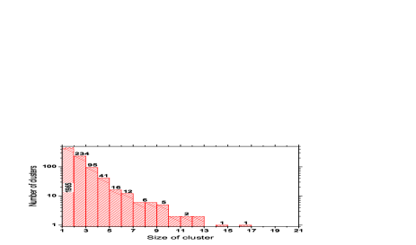
The 3691-triad cluster (monster) is not shown

${\mathcal{B}}$

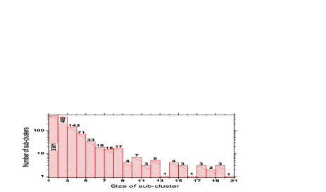
Sub-cl. size 21 24 28 30 32 33 35 37 38 44 121 127 130 Amount 2 3 1 1 1 2 1 1 1 1 1 1 2

Amount of sub-cluster of size $\geq 21$ shown in the table

Figure 6: Color online. Horizontal axes denote the number of triads in the cluster while vertical axes show the number of corresponding clusters (panel ${\mathcal{A}}$) and PP-irreducible subclusters (panel ${\mathcal{B}}$).

.

It can be seen that about $82.2\%$ of all clusters are presented by isolated triads and their dynamics has been investigated in KL-07 in all details; the main findings are that the energy oscillates between the three modes in the triads, with a period of oscillation that is much larger then the wave period. This period is inversely proportional to the root-mean-square of the wave amplitude.

234 clusters in the spectral domain ($\simeq 10.5\%$) are the butterflies discussed above; these are further analyzed below. Among them there are 131 PP-, 69 AP- and 35 AA-butterflies. The 95 triple-triad clusters include 25 ”triple-star” clusters with one triple connection, see Fig. 3. This set includes 3 AAA-, 5 AAP-, 6 APP- and 11 PPP-stars. There are also 66 chain clusters with two pair connections and 7 combinations of the connection types, shown in Fig. 4. We found also four (two pairs) triple-triad clusters with three pair connections, belonging to two different types, see Fig. 4.

Similar classification can be performed for all the other clusters. For example, the monster includes one mode (218,545), participating in 10 triads, three modes, participating in 9 triads, 5 modes – in 8 triads, 23 – in 7, 50 – in 6, 90 in 5, 236 – in 4, 550 – in 3 and 1428 modes – in 2 triads (butterflies). The analysis of their dynamical behavior depends crucially on the connection type as shown above and detailed below.

IV.2 PP-reduction of larger clusters

Large clusters can be divided into ”almost separated” subclusters connected by PP-connections (e.g. Figs. 5, 7 and 8). If such a sub-cluster cannot be divided further into smaller clusters connected by PP-connection we refer to it as a PP-irreducible cluster. For example, triangle cluster in Fig. 4 ${\mathcal{I}}$ can be PP-reduced to a triad and a PA-butterfly, while clusters in Fig. 8$\,{\mathcal{A}}$ and ${\mathcal{B}}$ can be PP-reduced to two and three individual triads respectively. The cluster in Fig. 7 is PP-reduced into three triads and PA-butterfly, while extended caterpillar in Fig. 5 is PP-reduced into three triads, PA-, AA-butterfly and AAA-star. One can see that the 14-triad cluster, shown in Fig. 9 ${\mathcal{A}}$ can be PP-reduced into 8 triads and 6-triad cluster. The 16-triad cluster (Fig. 9 ${\mathcal{B}}$) can be PP-reduced into 5 triads, AA- and PA-butterfly, AAP-star and 4-triad cluster, consisting of AAA-star with one AP-connected triad.

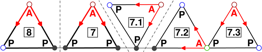
Figure 7: Color online. Triads $\Delta_{7}$ and $\Delta_{8}$, that belong to PP-butterfly $\bowtie_{7,8}$ are drawn by bold lines. New, connected to them triads $\Delta_{7.1}$, $\Delta_{7.2}$ and $\Delta_{7.3}$, appearing in spectral domain $m,\ell\leq 1000$ (for numeration of triads see Tab. 1), are drawn by thin lines. The PP-reduction of this cluster to three triads $\Delta_{7}$, $\Delta_{8}$ and $\Delta_{7.1}$ (according to the notation in Tab. 1) and one AP-butterfly is shown by dashed lines. The rest of notations as in Fig. 1.

${\mathcal{A}}$	${\mathcal{B}}$
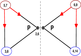
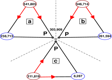
PP-reducible butterfly	PP-reducible

Figure 8: Color online. Examples of PP-reduction of pair connection, panel ${\mathcal{A}}$ and of triple connection, panel ${\mathcal{B}}$. Common (PP- and PPP-) modes are split stressing the difficulty of energy exchange between the corresponding triads. Dashed lines separate PP-irreducible sub-clusters, discussed in Sec. IV.2. The rest of the notations are as in Fig. 1.

${\mathcal{A}}$	${\mathcal{B}}$
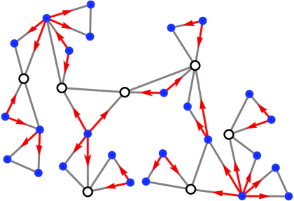
14-triad PP-reducible cluster	16-triad PP-reducible cluster

Figure 9: Large PP-reducible clusters. Common PP- and PPP-modes are shown by empty circles. The rest of modes are denoted by full (blue) circles. As in previous figures, outgoing (red) arrows indicate A-modes.

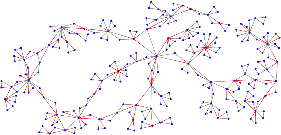
The 130-triad PP-irreducible sub-cluster belonging to the monster

Figure 10: Color online. Largest PP-irreducible cluster in the spectral domain $\ell,|m|\leq 1000$.

In the spectral domain $\ell,|m|\leq 1000$ the largest PP-irreducible sub-cluster belonging to the monster consists of 130 triads and is shown in Fig. 10. The statistics of PP-irreducible sub-clusters are presented in Fig. 6 ${\mathcal{B}}$.

We learn from this analysis that many clusters cannot carry energy flux through PP connections; their dynamics is naturally reduced to the dynamics of PP-irreducible sub-clusters. Therefore it is sufficient to study carefully the dynamics of these PP-irreducible clusters to understand the properties of any cluster.

V Numerical analysis of free evolution of typical sub-clusters

Our goal is to describe the energy flux through resonant triads in the regime of finite-dimensional wave turbulence. In the first Subsec. V.2 we consider free evolution of the smallest clusters – butterflies – from asymmetrical initial conditions, in which only one triad is excited to high amplitudes, exceeding by orders of magnitudes the initial amplitudes in the other triad. The questions are how the energy flux from the energetic “leading” triad depends on the type of connection, on the ratios of the interaction coefficients etc. Subsec. V.3 is devoted to the free evolution of the triple-triad clusters: stars and chains from initial conditions in which only the leading $a$-triad is substantially excited, the levels of excitation of the two other triads are much smaller. All these examples, and PA-PA-..PA chains, studied in the next Section, can serve as building blocks of bigger clusters and the knowledge about the energy flux through them allows to qualitatively predict efficiency of the energy transfer through bigger clusters.

V.1 Methodology and numerical procedure

The equations of motion for all clusters were prepared for numerical analysis using a specially designed algorithm that allowed an automatic implementation for any cluster, given the number of triads and the connectivity table. This served to avoid human errors in implementing large sets of equations.

The equations of motion for the free evolution of butterflies and triple clusters are stiff and were integrated using a multistep adaptive method based on numerical differentiation formulas num .

For each system of equations the accuracy of integration was controlled by testing the conservation of the relevant integrals of motion. The integration parameters were adjusted to keep the standard deviation $\sigma(I)$ below a given threshold for the duration of the numerical runs. Since the main parameter that affects the accuracy in terms of the conservation of the integrals of motion is the maximal allowed time step, the preliminary calculations were carried out with a requirement $\sigma(I)\leq 10^{-5}$; actually in most cases $\sigma(I)\leq 10^{-8}$ was achieved.

The evolution starting from several hundred initial conditions was analyzed and several representative conditions were chosen for the study of energy transfer in the clusters. All the conclusions regarding the discovered dependencies were verified by control calculations with stricter accuracy requirements.

The equation of motion for forced chain clusters, studied in the next Sec. VI, were integrated by both adaptive methods num and by 4th order constant time-step Runge-Kutta for better control of accuracy. By construction of the model, these equations required accurate description of the last triad in the cluster to ensure proper energy dissipation. The integration parameters were adjusted to reproduce this fastest evolution, and therefore were automatically suitable for all other triads. We verified the convergence of the resulting statistics with respect to all relevant parameters.

V.2 Free evolution in butterflies

The simplest topology that allows consideration of the energy flux between resonant triads is the double-triad clusters – butterflies.

V.2.1 Initial conditions, choice of the interaction coefficients and data representation

In this Subsection we show that details of the time evolution in butterflies are very sensitive to the initial conditions, which define the values of the dynamical invariants. Therefore a reasonable choice of initial conditions, allowing to shed light on a “typical” time evolution in a relatively compact form is not obvious. At initial time $t=0$ we assign most of the energy to two individual (not common) modes of one (leading) triad, denoted below for concreteness as $a$-triad. The initial amplitudes of these two modes we denote as $B_{0}$ and $\widetilde{B}_{0}$ (Fig. 2). To study the influence of the energy distribution between these modes we will use two types of initial conditions:

$$\mbox{Type I}: B_{0}=3.9+0.50~{}i\,,\ \widetilde{B}_{0}=3.7+0.93~{}i\,,~{}~{}~{}~{}~{}~{}$$ (34a)

$$\mbox{Type II}: B_{0}=5.3+0.50~{}i\,,\ \widetilde{B}_{0}=0.9+0.93~{}i\ .~{}~{}~{}~{}~{}~{}$$ (34b)

Both distributions (34) are complex and normalized such that $|B_{0}|^{2}+|\widetilde{B}_{0}|^{2}\approx 30$. The difference between Eq. (34a) and (34b) is that in Eq. (34a) both amplitudes are similar, while in Eq. (34b) they are quite different.

For different butterflies we choose in the leading triad:

PP-butterfly with $$B_{1|a}(0)=B_{1|b}(0):$$

$$B_{2|a}(0) = \widetilde{B}_{0}\,,\ B_{3|a}(0)=B_{0}\,;$$ (35a)

AA-butterfly with $$B_{3|a}=B_{3|b}:$$

$$B_{1|a}(0) = B_{0}\,,\ B_{2|a}(0)=\widetilde{B}_{0}\ ;$$ (35b)

PA-butterfly with $$B_{1|a}=B_{3|b}:$$

$$B_{2|a}(0) = \widetilde{B}_{0}\,,\ B_{3|a}(0)=B_{0}\,,$$ (35c)

as it is shown in Fig. 2.

The initial conditions in the driven $b$-triad we choose the same for all types of butterflies. They have much smaller initial amplitudes, for example:

$$\begin{cases}B_{1|b}(0)=B_{1,0}\,,\quad B_{1,0}\equiv C\,(0.05+0.02~{}i)\,,\\ B_{2|b}(0)=B_{2,0}\,,\quad B_{2,0}\equiv C\,(0.02+0.05~{}i)\,,\\ B_{3|b}(0)=B_{3,0}\,,\quad B_{3,0}\equiv C\,(0.10-0.02~{}i)\ .\end{cases}$$ (36)

To study the dependence of the energy flow between triads on the initial level of excitation of the driven triad we vary the energy content in the driven triad changing the coefficient $C$ in Eq. (36), taking in addition to $C=1$ also $C=0.1$ and $C=0.01$. In all the further simulations $C=1$ if else is not mentioned.

In this way the initial conditions for all butterflies are as similar as possible and we can study the difference in time evolutions, caused by different types of connections.

Last but not least are the interaction coefficients. For concreteness we chose interaction coefficients corresponding to $\Delta_{14}$ and $\Delta_{16}$ ($Z_{14}\approx 75$, and $Z_{16}\approx 15$) as prototypes and use either $\{Z_{a}=75\,,\ Z_{b}=15\}$ or vise versa and sometimes $\{Z_{a}=Z_{b}=15\}$. Since the change in the interaction coefficient re-normalizes the corresponding time scale, only their ratio is important for the dynamics. In our case these ratios are $=5\,,\ 1/5$ or $1$; this allows us to study the butterfly dynamics with very different values of the interaction amplitudes, which is typically the case. Having in mind that special choices of the ratios of interaction coefficients may lead to integrability of clusters of resonant triads ver (and see also 08-BK ) we verified that small variations of these ratios does not changed our conclusions concerning energy transfer in clusters.

Recall that any butterfly has three quadratic integrals of motion, that involve only squares of five amplitudes of modes and therefore only 2 combinations of them are independent. For the presentation we chose such combinations that are orthogonal to the corresponding invariants. Namely, for PP-butterflies, connected via $B_{1|a}=B_{1|b}$ modes:

$$J_{2,3|a}\equiv|B_{2|a}|^{2}-|B_{3|a}|^{2}\,,\quad J_{2,3|b}\equiv|B_{2|b}|^{2}-|B_{3|b}|^{2}\,;$$ (37a)

for AA-butterflies, connected via $$B_{3|a}=B_{3|b}$$ modes:

$$J_{1,2|a}\equiv|B_{1|a}|^{2}+|B_{2|a}|^{2}\,,\quad J_{1,2|b}\equiv|B_{1|a}|^{2}+|B_{2|b}|^{2}\,,$$ (37b)

and for AP-butterflies, connected via $B_{1|a}=B_{3|b}$ modes, $J_{2,3|a}$ and $J_{1,2|b}$.

Time evolutions for these three types of butterflies with various initial conditions and choices of the ratio $Z_{a}/Z_{b}$ (5 or 1/5) are shown in Figs. 11 – 15. Following Subsection V.2.3 is devoted to discussion of these numerical results.

V.2.2 Effect of the type of connections and of the ratio $Z_{a}\big{/}Z_{b}$

${\mathcal{A}}$	${\mathcal{B}}$
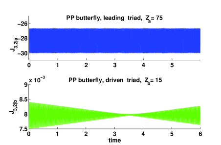
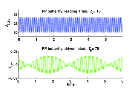
Blockade of the energy transfer in PP-butterfly	Blockade of the energy transfer in PP-butterfly
${\mathcal{C}}$	${\mathcal{D}}$
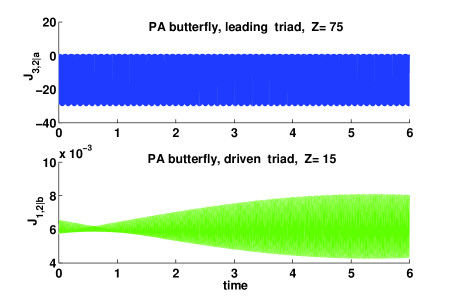
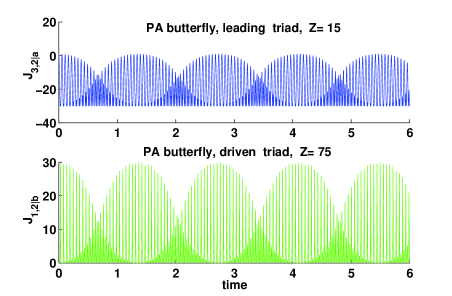
Strong suppression of the energy transfer in PA-butterfly	Efficient energy transfer in PA-butterfly
${\mathcal{E}}$	${\mathcal{F}}$
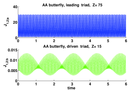
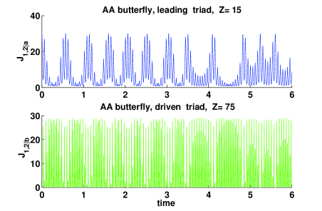
Strong suppression of the energy transfer in AA-butterfly	Efficient energy transfer in AA-butterfly

Figure 11: Color online. Time evolution of PP-, PA- and AA-butterflies with $Z_{a}=75$, $Z_{b}=15$, left panels and $Z_{a}=15$, $Z_{b}=75$, right panels. Initial conditions are given by Eqs. (34a), (35) and (36). In Figs. 11 – 16 time is measured in arbitrary units

${\mathcal{A}}$	${\mathcal{B}}$

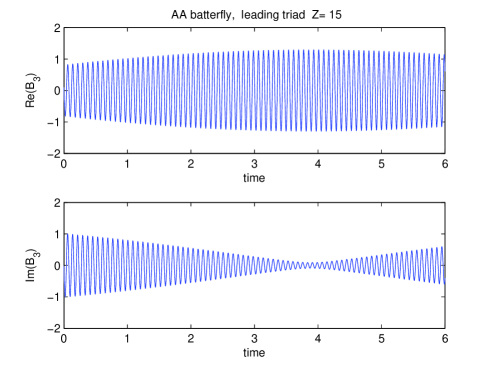
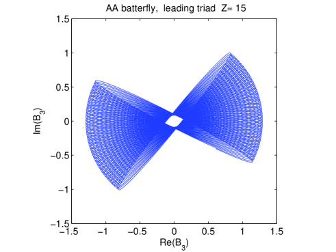
Figure 12: Time evolution of the common mode Re$B_{3|a}(t)$ and Im $B_{3|a}(t)$, panel ${\mathcal{A}}$, and the parametric representation Re$B_{3|a}(t)$ vs. Im $B_{3|a}(t)$, panel ${\mathcal{B}}$, for AA-butterfly with $Z_{a}=15\,,Z_{b}=75$ and the same initial conditions (34b), (35b) and (36) as in Fig. 11.

PP-butterfly

has the most trivial time-evolution, see Fig. 11 for $Z_{a}=75,\ Z_{b}=15$, (panel ${\mathcal{A}}$) and $Z_{a}=15,\ Z_{b}=75$, (panel ${\mathcal{B}}$). As expected, there is practically no energy exchange between triads: amplitudes $J_{2,3|a}\,,J_{2,3|b}$, defined by Eq. (37a), oscillate within the domains, that are determined by initial conditions. We show these evolutions just to illustrate our analytical result that PP-connection is non-penetrative for energy in both directions at any time.

AA-butterfly

is a promising candidate for the energy transfer. Time evolutions of $J_{1,2|a}(t)$ and $J_{1,2|a}(t)$ for AA-butterfly [defined by Eqs. (37b)] are shown in Fig. 11$\,{\mathcal{E}}\,,{\mathcal{F}}$. Indeed, as one sees in panel ${\mathcal{F}}$ the peaks of the amplitudes $J_{1,2|a}(t)$ in the leading triad and $J_{1,2|b}(t)$ in the driven triad are close to 30 for $Z_{a}=15,\ Z_{b}=75$. Quite unexpectedly, the energy transfer may be not efficient even with AA connections. Indeed, as one sees in Fig. 11 ${\mathcal{E}}$, when the leading $a$-triad has larger $Z_{a}=75$, the sum $|B_{1}|^{2}+|B_{2}|^{2}$ in the leading triad oscillates between $\approx 30$ and $\approx 20$ being close to its initial value $\approx 30$. At the same time, this sum in the driven triad oscillates close to its initial value $\approx 0.01$. Therefore the energy transfer is strongly suppressed if $Z_{a}\gg Z_{b}$.

To understand the difference between these two cases, consider time dependence of the common mode $B_{3}(t)$, for the case $Z_{a}=15\,,Z_{b}=75$ shown in Fig. 12 ${\mathcal{A}}$. One sees fast oscillations of the common mode $B_{3}(t)$ with (almost) zero mean and some frequency $\Omega_{a}$ that can be estimated as $Z_{a}B_{a}$, where $B_{a}\equiv\sqrt{J_{1,2|a}}$ is a characteristic value of mode magnitudes in $a-$triad. An illustration of this estimate one sees in Fig. 11 ${\mathcal{E}}$, where (for the same value of $|B_{a}|$) the oscillation frequency of the triads with $Z_{a}\approx 75$ is much higher than that for triads with $Z_{a}\approx 15$. As one can see from the equations of motion (25) for butterflies, the mean energy flux from the leading, $a-$, to the driven $b$-triad (with A-connection), $\varepsilon_{a\to b}$, can be written as

$$\varepsilon_{a\to b}=2Z_{b}\mbox{Re}\big{[}B_{1|b}B_{2|b}B_{3|b}^{*}\big{]}\propto\cos\phi_{b}\,,$$ (38)

where $\varphi_{b}=\varphi_{1|b}+\varphi_{2|b}-\varphi_{3|b}$ is the triad phase, introduces by Eq. (21b). Fast oscillations of $B_{a}(t)$, equivalent to fast growth of $\varphi_{3|b}(t)$ with the speed $d{\varphi}_{3|a}(t)/dt=d{\varphi}_{3|b}(t)/dt\approx\Omega_{a}(t)$ , lead to self-averaging of $\cos\varphi_{b}$ almost to zero, if phases $\varphi_{1|b}$ and $\varphi_{2|b}$ cannot react fast enough to variations of $\varphi_{3|b}(t)$. This is a qualitative explanation of the observed fact that the energy flux from $a-$ to $b-$triad is strongly suppressed if $Z_{a}\gg Z_{b}$ and is observable (but still suppressed) if $Z_{a}\lesssim Z_{b}$. One can hope that the $a-b$ energy flux can be significant if $B_{3|a}(t)$ has a nonzero mean and therefore $\langle\varphi_{3|b}(t)\rangle$ also does not vanish. But this is impossible under the initial conditions of interest: we do not want to put initially energy to $b-$triad, taking large value of $B_{3|a}(t)=B_{3|b}(t)$ at time zero. Therefore at $t=0$ $|B_{3|a}|\ll|B_{1|a}|,|B_{2|a}|$. If so, according to the equation of motion, the time derivative $\dot{B}_{3|a}=-Z_{a}B_{1|a}B_{2|a}$ is large enough to allow $B_{3|a}$ to cross quickly zero and to reach significant value with different sign. Having in mind periodical character of evolution of isolated triad it practically means that $\langle B_{3|a}\rangle\ll\sqrt{\langle|B_{3|a}|^{2}\rangle}$.

PA- and AP-butterflies.

Considering free evolution from asymmetrical initial conditions we will distinguish PA-butterfly, in which the leading triad has P-connection and the driven triad has A-connection, from AP-butterfly, in which the leading triad has A-connection and the driven triad has P-connection.

We found that in AP-butterflies the energy transfer to the driven triad is blocked by the second of the conservation laws (27b) and its evolution is similar to that of PP-butterfly.

On the contrary, PA-butterflies demonstrate time evolution similar to that of AA-butterflies: compare in Fig. 11 panels ${\mathcal{C}}$ and ${\mathcal{D}}$ for PA-butterfly with panels ${\mathcal{E}}$ and ${\mathcal{F}}$ for AA-butterflies. One sees that corresponding plots in both panels are quantitatively the same: in the left panels (with $Z_{a}=75\,,\ Z_{b}=15$) the energy transfer is strongly suppressed (with $J\sim 0.01$ in the driven triad), while in the right panels (with $Z_{a}=15\,,\ Z_{b}=75$) the energy transfer is efficient (with $J\sim 10\div 30$ in the driven triad).

To complete discussion on how the energy transfer depend on the ratio $Z_{a}\big{/}Z_{b}$ we present in Fig. 13 time evolution from the same as in Fig. 11 initial conditions, but with equal values of the interaction coefficients, taking for concreteness $Z_{a}=Z_{b}=15$. The excitation level of the driven triad $J_{1,2|b}\simeq 0.2$. As expected, this level is larger than $\simeq 0.01$ for $Z_{a}\big{/}Z_{b}=5$ and smaller than $\simeq 20$ for $Z_{a}\big{/}Z_{b}=1/5$.

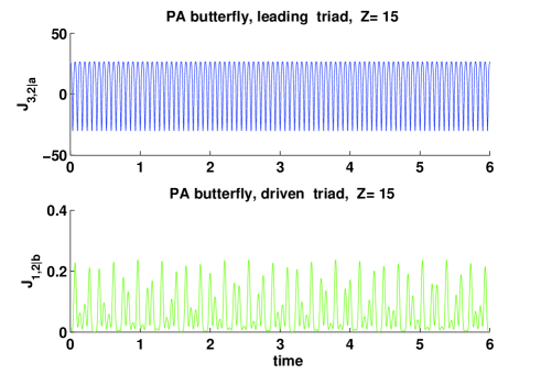
Figure 13: Color online. Suppression of the energy transfer in PA-butterfly with equal values of the interaction coefficients: $Z_{a}=Z_{b}=15$. Initial conditions are the same as in Fig. 11 for PA-butterfly: Eqs. (34a), (35c) and (36).

${\mathcal{A}}$

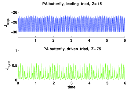
${\mathcal{B}}$

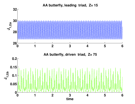
Figure 14: Color online. Suppression of the energy transfer by initial conditions in PA- and AA butterflies.

${\mathcal{A}}$	${\mathcal{B}}$
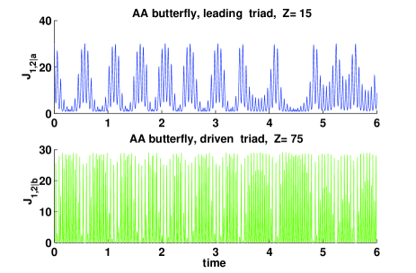
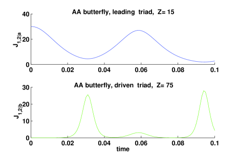
Long time evolution for $C=1\,,0.1$ and $0.01$	Initial stage of the evolution with $C=1$.
${\mathcal{C}}$	${\mathcal{D}}$
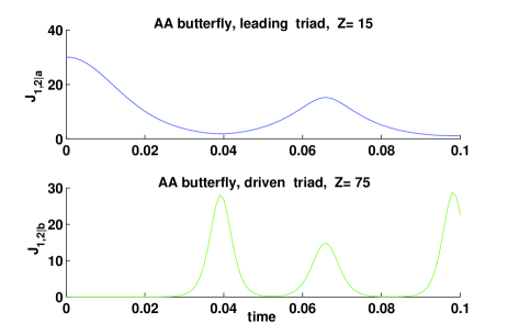
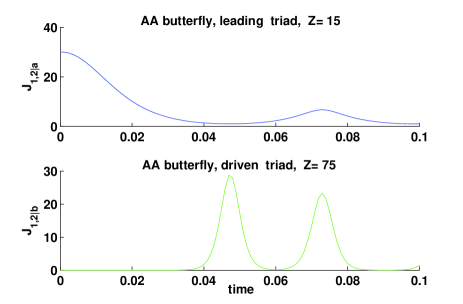
Initial stage of the evolution with $C=0.1$	Initial stage of the evolution with $C=0.01$

Figure 15: Color online. Time evolution of AA-butterfly with different level of excitation in the driven triad, governed by parameter $C$ in Eq. (36).

V.2.3 Effect of initial conditions

As we mentioned, the time evolution and efficiency of the energy transfer between triads crucially depend on the initial conditions. To demonstrate this we present in Fig. 14 the evolution of PA-butterflies ( panel ${\mathcal{A}}$) and AA-butterflies (panel ${\mathcal{B}}$) for the same “efficient” values of the interaction coefficients ($Z_{a}=15,\ Z_{b}=75$), as in Fig. 11$\,{\mathcal{D}}$, ${\mathcal{E}}$ and ${\mathcal{F}}$. The only difference is in initial conditions, that on the first glance are very similar to that used above in Fig. 11. Namely, for PA-butterflies we simply interchange initial amplitudes of individual modes in the leading $a$-triad, replacing $B_{0}\Leftrightarrow\widetilde{B}_{0}$ in Eq. (35c). For AA-butterflies we replace almost equal values of $B_{0}$ and $\widetilde{B}_{0}$ in Eq. (34a) by different in an order of magnitude values (34b) with the same sum $|B_{0}|^{2}+|\widetilde{B}_{0}|^{2}\approx 30$. The result of this “minor” change is crucial: in PA-butterfly the excitation level $J_{1,2|b}$ decreases from $\simeq 20$ to $\simeq 0.4$ and in AA-butterfly from from $\simeq 20$ to $\simeq 0.1$.

In order to rationalize this effect notice that the energy flux from the $a$- to $b$-triad is proportional to the level of excitation of the common mode, $\langle|B_{3|b}|^{2}\rangle$ for both butterflies under consideration. To estimate the upper bound for $\langle|B_{3|b}|^{2}\rangle$ we can approximate $a$-triad as an isolated one, neglecting the feedback effect of the driven triad on the leading one. In this approximation we can use the invariants (19) for isolated triad:

$$I_{1,3|a}=|B_{1|a}|^{2}+|B_{3|a}|^{2}\!\!,\ I_{2,3|a}=|B_{2|a}|^{2}+|B_{3|a}|^{2}.~{}~{}$$ (39)

AA-butterfly.

In AA-butterfly initially the amplitude $|B_{3|a}|\ll|B_{1|a}|,\ |B_{2|a}|$. Therefore $I_{1,3|a}=|B_{1|a}(t=0)|^{2}\equiv|B_{1|a}^{\,(0)}|^{2}$ and $I_{2,3|a}=|B_{2|a}^{\,(0)}|^{2}$ and thus

$$\begin{cases}|B_{3|a}|^{2}\leq|B_{1|a}^{\,(0)}|^{2}\\ |B_{3|a}|^{2}\leq|B_{2|a}^{\,(0)}|^{2}\\ \end{cases}\!\!\!\!\!\!\!\! \Rightarrow \!\!\!|B_{3|a}|^{2}\leq\min\{|B_{1|a}^{\,(0)}|^{2},|B_{2|a}^{\,(0)}|^{2}\}.~{}~{}~{}~{}~{}~{}$$ (40)

This means that the efficiency of the energy transfer is determined by the smallest initial magnitudes of the individual modes; fixing sum of their squares one has the most efficient transfer at (almost) equal initial magnitudes. This was realized in the first version of the initial conditions (34a), that leads to the best energy transfer, in which, according to Fig. 11$\,{\mathcal{F}}$ $\max{J_{1,2|b}}\approx 30$.

Let us show, that this is indeed the maximal possible value of the level of excitation of the driven triad $J_{1,2|b}$. To this goal consider the invariants (27c) of AA-butterfly, that can be combined as follows:

$$I_{\scriptscriptstyle\rm{AA}}=|B_{1|a}|^{2}+|B_{2|a}|^{2}+2|B_{3|a}|^{2}+|B_{1|b}|^{2}+|B_{2|b}|^{2}\ .$$ (41a)

At $$t=0 B_{1|a}=B_{0} B_{2|a}=\widetilde{B}_{0} I_{\scriptscriptstyle\rm{AA}}=B_{1|a}|^{2}+|B_{2|a}|^{2}=J_{1,2|a}=|B_{0}|^{2}+|\widetilde{B}_{0}|^{2}$$ , (or vise versa) and much larger than the rest of the amplitudes. Therefore and thus

$$J_{1,2|b}\simeq|B_{1|b}|^{2}+|B_{2|b}|^{2}\leq I_{\scriptscriptstyle\rm{AA}}\approx 30\,,\quad\mbox{AA.}$$ (41b)

Finally notice, that in view of the restriction (40) it is clear, that with the second choice of the initial conditions (34b) the energy transfer should be much less efficient. This is exactly what one sees in Fig. 14$\,{\mathcal{B}}$.

PA-butterfly.

The situation is a bit different for PA-butterfly with P- and A-modes being individual in the leading $a$-triad. In this case combining invariants (27b) for PA-butterfly one finds new (dependent) invariants:

$$I_{\scriptscriptstyle\rm{PA}} = |B_{3|a}|^{2}-|B_{2|a}|^{2}+2|B_{3|b}|^{2}+|B_{1|b}|^{2}~{}~{}~{}~{}$$

$$+|B_{2|b}|^{2}=J_{3,2|a}+J_{1,2|b}+2|B_{3|b}|^{2}\ .$$

At $$t=0 B_{2|a}=\widetilde{B}_{0} B_{3|a}=B_{0} I_{\scriptscriptstyle\rm{PA}}=J_{2,3|a}(0) -(|B_{0}|^{2}-|\widetilde{B}_{0}|^{2}) I_{\scriptscriptstyle\rm{PA}}=|B_{0}|^{2}-|\widetilde{B}_{0}|^{2}$$, , (or vise versa) and much larger than the rest of the amplitudes. Therefore which is equal to for the old initial conditions and to for the new ones. This allows one to write:

$$I_{\scriptscriptstyle\rm{PA}}=J_{2,3|a}(0)\approx\pm 26.7\,,\ \mbox{PA.}$$ (42b)

Unfortunately, in this case invariant $I_{\scriptscriptstyle\rm{PA}}$ is not positive definite and therefore one cannot get rigorous restriction on $J_{1,2|b}$, similar to (41b). Nevertheless, more detailed analysis allows us to think that the upper bound for $J_{1,2|b}$ for PA-butterfly should be the same as for AA-butterfly, i.e. about 30 for our initial conditions.

In order to clarify the dependence of the energy transfer on initial conditions we should estimate the amplitude of common mode similarly to the case of AA-butterfly, neglecting the excitation of the driven triad. In this case invariants (27b) can be written as:

$$I_{1,3|a}=|B_{1|a}|^{2}+|B_{3|a}|^{2}\!\!,\ I_{1,2|a}=|B_{1|a}|^{2}-|B_{2|a}|^{2}.~{}~{}$$ (43)

At initial moment of time the amplitude $|B_{1|a}|\ll|B_{2|a}|,\ |B_{3|a}|$. Therefore $I_{1,3|a}\simeq|B_{3|a}(t=0)|^{2}\equiv|B_{3|a}^{\,(0)}|^{2}$ and $I_{3,2|a}=|B_{3|a}^{\,(0)}|^{2}-|B_{2|a}^{\,(0)}|^{2}$. Thus the first of Eqs. (43) gives

$$|B_{1|a}|^{2}=|B_{3|b}|^{2}\leq|B_{3|a}^{\,(0)}|^{2}\,,$$ (44)

while the second one leads to the trivial restriction $|B_{1|a}|^{2}\geq-|B_{3|a}^{\,(0)}|^{2}$, that is satisfied automatically. The conclusion is that the efficiency of the energy transfer is determined by the initial magnitudes of the individual A-mode. This was realized in the first version of the initial conditions in which we assigned more energy to $B_{3|a}$ mode; that leads to the best energy transfer.

The next question is how to rationalize why the energy transfer into the driven triad can exceed 50%. Intuitively the answer is rather obvious: we understood already that the energy transfer is much more effective, if the accepting triad has larger interaction coefficient $Z$. Therefore in the considered case, when $Z_{b}\gg Z_{a}$, during long evolution with various values of the triad phase (that determines the direction of the energy flux) and with similar value of the triad excitations, the energy flux from $a$- to $b$-triad is more favorable than the flux in the opposite direction. This leads to the asymmetry of the mean energy content between triads in favor of the $b$-triad with larger value of the interaction coefficient: $Z_{b}\gg Z_{a}$.

What depends on the excitation level of the driven triad?

Up to now we have considered initial conditions in the leading triad, just by mentioning that the driven triads have much smaller values of the initial excitations. The reason for this neglect is that the time evolution is insensitive to the initial excitations in the driven triads, their level just have to be very small. To demonstrate this we compare the time evolution of AA-triad with $Z_{a}=15$, $Z_{b}=75$ from the initial conditions (34a), (35b) and with “standard” level of initial excitation in $b$-triad [$C=1$ in Eqs. (36)] with that for the much smaller initial energy contents in the driven triad, see Fig. 15. The long-time evolution is practically independent of $C$ as shown in Fig. 15$\,{\mathcal{A}}$. The $C$-dependence is visible only on the initial stages of the evolution: panel-${\mathcal{B}}$ with $C=1$, -${\mathcal{C}}$ with $C=0.1$ and -${\mathcal{D}}$ with $C=0.01$. One sees that the position of the first maximum for $C=1$ is at $t_{\text{max}}\approx 0.03$, for $C=0.1$ at $t_{\text{max}}\approx 0.04$, while for $C=0.01$ at $t_{\text{max}}\approx 0.05$. This dependence is quite understandable: according to Eqs. (25b) initial small perturbations in the driven triad grow exponentially in time due to the parametric instability of the common $B_{3|b}$ mode with respect of decay into small individual modes: $B_{1|b}\,,\ B_{2|b}\propto\exp(Z_{b}|B_{3|b}|t)$ modes. Therefore

$$t_{\text{max}}\propto-\ln Z_{b}C\,,$$ (45)

as observed.

${\mathcal{A}}$	${\mathcal{B}}$
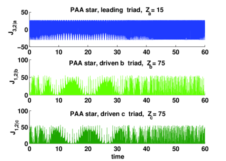
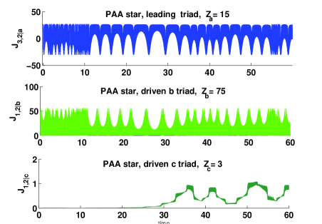
Efficient energy transfer from $a$- to $b$-triad ($Z_{b}/Z_{a}=5$)         and from $a$- to $c$-triad ($Z_{c}/Z_{a}=5$)	Efficiency of the energy transfer from $a$-triad to        $b$-triad ($Z_{b}/Z_{a}=1/5$) is a bit smaller than that        to $c$-triad ($Z_{c}/Z_{a}=5$)
${\mathcal{C}}$	${\mathcal{D}}$
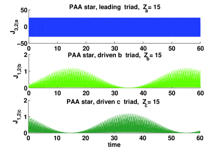
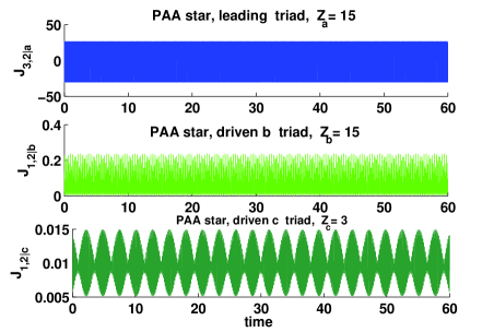
Suppression of the energy transfer in PAA-star        junction with $Z_{a}=Z_{b}=Z_{c}$	Strong suppression of the energy transfer in PAA-star        junction with $Z_{a}=Z_{b}>Z_{c}=3$

Figure 16: Color online. Efficiency of PAA-star energy junction with different $Z_{b}/Z_{a}$ and $Z_{c}/Z_{a}$ [initial conditions (46)].

${\mathcal{A}}$	${\mathcal{B}}$
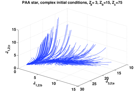
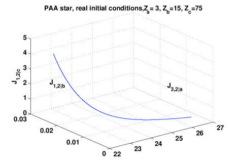
${\mathcal{C}}$	${\mathcal{D}}$

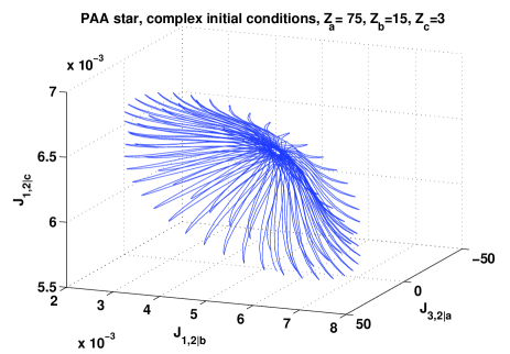
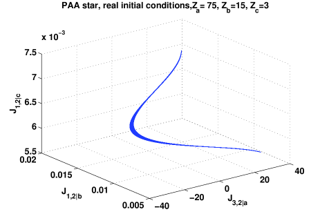
Figure 17: Color online. Three dimensional parametric representation of trajectories of PAA-star with $Z_{a}=3$, $Z_{b}=15$, $Z_{c}=75$, panels ${\mathcal{A}}$ and ${\mathcal{B}}$ and with $Z_{a}=3$, $Z_{b}=15$, $Z_{c}=75$, panels ${\mathcal{C}}$ and ${\mathcal{D}}$. Left panels: Complex initial conditions (46); Right panels: real initial conditions in which complex number in Eq. (46) are replaced by their absolute values.

${\mathcal{A}}$	${\mathcal{B}}$

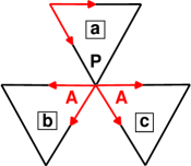
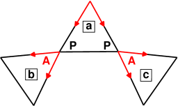
Figure 18: Triple-star (${\mathcal{A}}$) and triple-chain (${\mathcal{B}}$) energy junctions. Initial energy is localized in the leading $a$-triad and goes during free evolution in two driven $b$- and $c$-triads.

V.3 Energy-junctions in the triple-triad clusters

In this Subsection we study free evolution of the triple-triad clusters, that allow to shed light on the energy transfer from one triad to two other triads. To this aim we consider here free evolution of various triple-triad clusters, in which the leading $a$-triad will be initially highly exited, while the level of excitation of two other $b$- and $c$-triads will be relatively small. One topological option for effective energy flux from $a$- to $b$- and $c$-triad, considered in the next Sec. V.3.1 is PAA-star. One more option is the triple-triangle configuration, in which energy goes from one triad to two other, PP-connected triads. This structure is very rare and will not be discussed here. Next option, considered in Sec. V.3.2, is AP-PA chain with the leading $a$-triad in the middle.

${\mathcal{A}}$	${\mathcal{B}}$
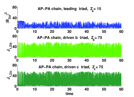
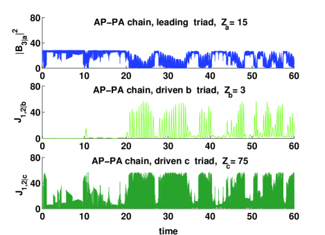
Efficient energy transfer from $a$- to $b$-triad ($Z_{b}/Z_{a}=5$)        and from $a$- to $c$-triad ($Z_{c}/Z_{a}=5$), similar to that        in PAA-star in the same panel in Fig. 16.	The energy transfer from $a$-triad to $b$-triad is very        intermittent, but much more efficient than that        in PAA-star
${\mathcal{C}}$	${\mathcal{D}}$
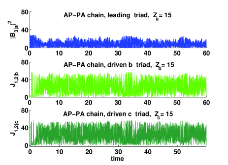
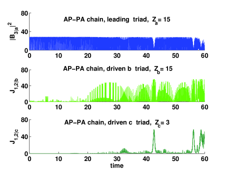
Efficient energy transfer for AP-PA chain        with $Z_{a}=Z_{b}=Z_{c}$, unlike PAA-star	Efficient energy transfer for AP-PA chain        with $Z_{a}=Z_{b}>Z_{c}$, unlike PAA-star

Figure 19: Color online. Efficiency of AP-PA-chain energy junction with different $Z_{b}/Z_{a}$ and $Z_{c}/Z_{a}$ [initial conditions (47)].

V.3.1 Triple-star junction

An effective component in the energy transfer through big clusters is the PAA-star. PAA-star can accept energy via A-mode of $a$-triad and transfer it to two other $b$- and $c$-triads, via their A-modes, $B_{3|b}$ and $B_{3|c}$, connected to the (same) passive $B_{1|a}$ mode of the $a$-triad (see Fig. 18, ${\mathcal{A}}$). In order to clarify how an additional $c$-triad affects the energy in PA-butterfly studied above, we present in Fig. 16 an evolution of PAA-star with the choice of the interaction coefficients similar to that of above and with “energy-transfer effective” initial conditions, given by Eq. (35c) in $a$-triad, Eq. (36) in $b$-triad. For $c$-triad we took initial conditions similar to that for $b$-triad Eq. (36), but with the complex conjugated $B_{1,0}$ and $B_{2,0}$. Hence, the initial conditions are as follows:

$$\begin{cases}B_{1|a}(0)=B_{3|b}(0)=B_{3|c}(0)=B_{3,0}\,,\\ B_{2|a}(0)=\widetilde{B}_{0}\,,\qquad\ B_{3|a}(0)=B_{0}\,;\end{cases}$$ (46a)

$$~{}~{}B_{1|b}(0)=B_{1,0}\,,\qquad B_{2|b}(0)=B_{2,0}\,;$$ (46b)

$$~{}~{}B_{1|c}(0)=B_{1,0}^{*}\,,\qquad B_{2|c}(0)=B_{2,0}^{*}\ .$$ (46c)

Quite expectedly, when the leading triad has much smaller interaction coefficient than the driven ones (see Fig. 16$\,A$ with $Z_{a}\ll Z_{b}=Z_{c}=75$), the energy transfer to both driven triads is fully effective. The new element with respect to the butterfly case is the energy oscillation between driven triads.

Panel ${\mathcal{B}}$ in Fig. 16 demonstrates an evolution of the PAA-star, in which driven $c$-triad has the interaction coefficient $Z_{c}=3$, i.e. five times smaller than in the leading triad. As expected, the energy transfer to very slow $c$-triad is strongly suppressed, below the level $J_{1,2|c}\lesssim 1$.

The same level of excitation, $J_{1,2|b}\approx J_{1,2|c}\lesssim 1$ demonstrates the PAA-star with all equal interaction coefficients, see Fig. 16$\,{\mathcal{C}}$. The energy alternations between equivalent triads is even more pronounced, than in case $Z_{a}\ll Z_{b}=Z_{c}=15$, that demonstrates a more stochastic behavior.

The comparison of Fig. 16$\,{\mathcal{B}}$ and $\,{\mathcal{D}}$ shows that the decrease in $Z_{b}$ (from 75 to 15) suppresses energy transfer to the $c$-triad even further up to level $0.015\ll 1$.

The overall conclusion is that qualitatively the difference in the interaction coefficients affects the energy transfer in triple stars similarly to that in butterflies, but on the quantitative level the interplay of two driven triads cannot be neglected.

Another expected conclusion is that the triple clusters demonstrate “more random” evolution than butterflies. However, the level of randomness strongly depends on the initial conditions. One sees this from three-dimensional parametric representation of PAA-star trajectories in Fig. 17 with different choice of the interaction coefficients in the upper and lower panels. Left panels shows randomization of trajectories, starting from complex initial conditions (46), right panels – much more regular behavior of the trajectories, starting from similar, but real initial conditions (in which complex number in Eq. (46) are replaced by their absolute values). The qualitative explanations of this difference is very simple. Equations of motion for triple stars (29) are real. Therefore the mode amplitudes $B_{\dots}$, that start from the real initial conditions, remain real during the evolution and the dimensionality of the phase space in that case is smaller than that during evolution from general (complex) initial conditions. Note also that the real trajectories, although close to periodical ones, have small random components that lead to the finite “width” of the attractors in Eq. (46), right panels.

V.3.2 AP-PA-chain energy junction

Another example of an effective energy junction is the triple AP-PA-chains, in which energy can be accepted via A-mode of the middle $a$-triad and transferred to other two $b$- and $c$-triads via their A-modes, $B_{3|b}$ and $B_{3|c}$, connected to different P-modes of the $a$-triad from the left and the right: $B_{3|b}=B_{1|a}$ and $B_{3|c}=B_{2|a}$ (see Fig. 18, ${\mathcal{B}}$). A choice of the initial conditions that guarantees efficiency of the energy transfer is similar to Eqs. (46) with the differences that are dictated by different types of the connections:

$$\begin{cases}B_{1|a}(0)=B_{3|b}(0)=B_{3,0}\,,\\ B_{2|a}(0)=B_{3|c}(0)=B_{3,0}^{*},\quad B_{3|a}(0)=B_{0}\,;~{}~{}~{}\end{cases}$$ (47a)

$$~{}~{}B_{1|b}(0)=B_{1,0}\,,\qquad B_{2|b}(0)=B_{2,0}\,;$$ (47b)

$$~{}~{}B_{1|c}(0)=B_{1,0}^{*}\,,\qquad B_{2|c}(0)=B_{2,0}^{*}\ .$$ (47c)

In Fig. 19 we show the time evolution of the triple AP-PA-chain with the same four sets of the interaction coefficients, as in Fig. 16 for APP-stars.

Comparing Fig. 19 with Fig. 16 panel by panel one concludes, that the triple AP-PA-chain, in which the driven triads are connected to different modes of the leading triad, demonstrates much more efficient energy transfer, than the triple PAA-star, in which the driven triads are connected to the same mode of the leading triad. Another difference, is that the time evolution in the triple AP-PA-chain is much more intermittent than in the triple PAA-star.

VI Finite-dimensional wave turbulence in the long-chain clusters

In this Section we study stationary energy distributions of resonant waves and energy exchange between triads in the long-chain clusters in the regime of finite-dimensional wave turbulence with constant energy flux and during free evolution.

VI.1 Pumping and damping in chain clusters

With this subsection we begin to consider the stationary dynamics of the $N$-chain clusters, consisting of many resonant triads (with $N=12,16,20$ and $24$). To do this numerically one should model the energy pumping in the leading $a$-triad and energy dissipation in the driven $N^{\rm th}$-triad.

The simplest and reasonable way to model the energy dissipation is quite obvious: one should introduce linear damping terms into the equations of motion for individual modes of the last driven triad. In our case these are P-modes and instead of Eqs. (25c) we suggest the following two equations for them:

$$\begin{cases}\dot{B}_{1|N}=Z_{N}B_{2|N}^{*}B_{3|N}-\gamma_{1|N}{B}_{1|N}\,,\\ \dot{B}_{2|N}=Z_{N}B_{1|N}^{*}B_{3|N}-\gamma_{2|N}{B}_{2|N}\,,\end{cases}$$ (48)

with some phenomenological damping frequencies $\gamma_{1|N}$ and $\gamma_{2|N}$ that should be compared with the characteristic interaction frequency in these equations

$$\Omega_{\rm int|N}\equiv Z_{N}\sqrt{\langle|B_{3|N}|^{2}\rangle}\ .$$ (49)

Then one can distinguish the cases of symmetrical damping: $\gamma_{1|N}=\gamma_{2|N}$, asymmetrical damping: $\gamma_{1|N}\neq\gamma_{2|N}$, but $\gamma_{1|N}\simeq\gamma_{2|N}$ and strong damping asymmetry: $\gamma_{1|N}\gg\gamma_{2|N}$. In addition there are cases of weak damping, when $\displaystyle\sqrt{\gamma_{1|N}\gamma_{2|N}}\ll\Omega_{\rm int|N}$, intermediate and strong damping, when $\displaystyle\sqrt{\gamma_{1|N}\gamma_{2|N}}\approx\Omega_{\rm int|N}$ and $\displaystyle\sqrt{\gamma_{1|N}\gamma_{2|N}}\gg\Omega_{\rm int|N}$. To start with in this paper we will restrict ourselves by the simplest case of weak symmetrical damping.

In all cases we will include energy pumping term $P_{3|1}$ in the equation of motion for the A-mode of the first (leading) triad, i.e. in the equation for $B_{3|a}$. Now it reads:

$$\dot{B}_{3|1}=-Z_{1}B_{1|1}B_{2|a}+P_{3|1}\ .$$ (50)

How to mimic energy pumping is a much more delicate question. Notice, that in the problems of developed wave or hydrodynamic turbulence researches usually fill free to model the energy source and sink in the simplest possible manner 95LP . For example, one introduces a random force with Gaussian statistics (that has some justification) and $\delta$-correlated in time, which is usually far from reality, see e.g. Fri . The rationale is that for very high levels of turbulence excitation the inertial interval of scales is large enough such that one expects universal statistics of turbulence, independent of characteristics of the energy pumping 95LP . In our case of relatively low level of excitation, when the number of excited degrees of freedom is not so huge, the universality is, generally speaking, questionable: statistics of the system dynamics can depend on the way the system is excited. One can imagine few very different versions of the pumping term.

The first version mimics an instability of the $B_{3|1}$ mode with an inverse growth time $\nu_{(3|1)}$ :

$$P_{3|1}=\nu_{{3|1}}B_{3|1}\,,$$ (51a)

Next one can consider a periodic driving force:

$$P_{3|1}=F_{\omega}\cos(\omega t)\,,$$ (51b)

that can mimic the effect of an “external” triad, connected to $B_{3|1}$ mode. In this case $\omega$ is the leading frequency of energy exchange between modes of the external triad.

Also one can take a random white Gaussian noise

$$P_{3|1}=f(t)\,,\quad\langle f(t)f(t^{\prime})\rangle=f^{2}\delta(t-t^{\prime})\,,$$ (51c)

that mimics the influence of numerous non-resonant triads.

In this paper we will utilize a bit more realistic driving force $P_{3|a}(t)$ [periodic, but not $\propto\cos(\omega t)$, as in Eq. (51b)] that is produced by the equations of motion for an isolated triad. This mimics the effect of an “external” triad, connected to $B_{3|a}$ mode in the approximation, when the feedback effect is neglected.

VI.2 Condition of stationarity

Consider first the dynamical invariants for isolated $N$-chain clusters (without pumping and damping terms). Combining invariants (19), one has in this case a (dependent) invariant for isolated triad in the form

$$I_{|1}=|B_{3|1}|^{2}+\frac{1}{2}\big{(}|B_{1|1}|^{2}+|B_{2|1}|^{2}\big{)}\ .$$ (52a)

Similarly, a combination of invariants (27b) yields the invariant for PA-butterfly:

$$I_{|1,2}=|B_{3|1}|^{2}+|B_{3|2}|^{2}+\frac{1}{2}\big{(}|B_{1|2}|^{2}+|B_{2|2}|^{2}\big{)}\ .$$ (52b)

And finally, from invariants (31c) one derives new (dependent) invariant for PA-PA-chain:

$$I_{|1,2,3}=|B_{3|1}|^{2}+|B_{3|2}|^{2}+|B_{3|3}|^{2}+\frac{1}{2}\big{(}|B_{1|3}|^{2}+|B_{2|3}|^{2}\big{)}\ .$$ (52c)

Similarly, for isolated $$N$$-chain cluster one gets:

$$I_{|1,2,\dots N}=\sum_{j=1}^{N}|B_{3|j}|^{2}+\frac{1}{2}\big{(}|B_{1|N}|^{2}+|B_{2|N}|^{2}\big{)}\ .$$ (52d)

All these invariants include $B_{3|1}$-mode, affected by the pumping, and $\frac{1}{2}\big{(}|B_{1|N}|^{2}+|B_{2|N}|^{2}\big{)}$ terms, affected by the damping. Therefore under the stationary conditions the following equality must hold:

$$\langle P_{3|1}B_{3|1}^{*}\rangle=\frac{1}{2}\big{(}\gamma_{1|N}\langle|B_{1|N}|^{2}\rangle+\gamma_{2|N}\langle|B_{2|N}|^{2}\rangle\big{)}\ .$$ (53a)

In particular for the pumping (51a) one has a simple relationship:

$$\gamma_{3|1}\langle|B_{3|1}|^{2}\rangle=\frac{1}{2}\big{(}\gamma_{1|N}\langle|B_{1|N}|^{2}\rangle+\gamma_{2|N}\langle|B_{2|N}|^{2}\rangle\big{)}\ .$$ (53b)

Equations (53) can be considered as the (nessesary) condition of the energy balance: the left hand side describes the energy pumping, while the right had side – the energy damping. Each of these quantities can be equated (under the stationary conditions) to the energy flux through the clusters.

VI.3 Universality of statistics of finite-dimensional wave turbulence in the long-chain clusters

VI.3.1 Modeling the parameters of the forced chain clusters

We present here our choice of the modeling parameters for the forced PA-PA-…-PA chain clusters. The cluster consists of $N$ triads and is constructed by connecting the first P-mode of $(n-1)$’s triad, $B_{1|n-1}$, with the A-mode of the next, $n$’s triad, $B_{3|n}$. The interaction coefficients $Z_{n}$ were chosen in geometric progression,

$$Z_{n}=\lambda Z_{n-1}=Z_{1}\lambda^{n-1}\,.$$ (54)

The chain is forced by an independent freely evolving triad with $Z_{0}=0.125$ related to $Z_{1}$ as $Z_{1}=Z_{0}\lambda$. The amplitude $B_{1|0}$ of the forcing triad is added to the equation of $B_{3|1}$ of the first triad in the chain 200 times during the period $T_{f}$ of the forcing triad. We made special efforts to ensure the exact periodicity of the forcing.

The linear dissipation with the damping frequency $\gamma$ was added to the equations of two P-modes of the last triad, $B_{1|N}$ and $B_{2|N}$. In most calculations $\gamma=10^{-4}$ was used.

We have studied the mean square amplitudes of “free” modes, $\langle|B_{2|n}|^{2}\rangle$ and “connected” modes $\langle|B_{3|n}|^{2}\rangle=\langle|B_{1|n-1}|^{2}\rangle$ in the chains with different number of triads, $N=16,\ 20,\ 24$, for the set of the frequency scaling parameter $\lambda=1,\ \sqrt{2},\ 2,\ 2\sqrt{2}$ and using different initial conditions in the pumping triad.

We found that initial conditions do not effect the stationary statistics in the cluster. For concreteness, for all presented simulations we chose for the pumping triad

$$B_{1|0} = 0.05+0.02\,i\,,$$ (55)

$$B_{2|0} = 0.02+0.05\,i\,,$$ (56)

$$B_{3|0} = 0.9-0.93\,i\,;$$

and for all $N$ triads of the chain

$$B_{1|n} = 0.05+0.02\,i\,,$$ (57)

$$B_{2|n} = 0.02+0.05\,i\,,$$ (58)

$$B_{3|n} = B_{1|n-1}\ .$$

The time of the chain evolution required to reach stationarity varied from about 1000 $T_{f}$ of the pumping triad for $\lambda=1$ to about 50 $T_{f}$ for $\lambda=2\sqrt{2}$. For times later than 1000 $T_{f}$ we calculated mean values in time, averaging values of $\langle|B_{j|n}|^{2}\rangle$ over $300T_{f}$. In the most fast converging case of $\lambda=2\sqrt{2}$ we averaged over $50T_{f}$. In all cases the evolution was followed for much longer times and we verified that a particular choice of the averaging interval does not affect results.

Our results are presented in Figs. 20 as logarithm of $\langle|B_{2|n}|^{2}\rangle$ and $\langle|B_{3|n}|^{2}\rangle$, normalized by its value in the first triad vs triad number $n$ normalized by $N$. To force all lines to start from the same point and not from $1/N$, we shifted triad numbers by $1$: $n\to n-1$ for presentation. Such a shift leads to better collapse of the data.

VI.3.2 $N$-, $\lambda$- and $\gamma$-independence of the forced-chain statistics

Figure 20$\,{\mathcal{A}}$ presents normalized mean-square amplitudes $\langle|B_{2|n}|^{2}\rangle$ and $\langle|B_{3|n}|^{2}\rangle$ for the chain with $N=16$ and a set of the scaling parameters $\lambda=1,\ \sqrt{2},\ 2$ and $\lambda=2\sqrt{2}$. One sees that the lines for different $\lambda$ are quite close, quickly converging for larger $\lambda$. We conclude that the distributions of $\langle|B_{2|n}|^{2}\rangle$ and $\langle|B_{3|n}|^{2}\rangle$ are almost $\lambda$-independent at least for $\lambda\geq 2$.

Figure 20$\,{\mathcal{B}}$ represents distributions of $\langle|B_{2|n}|^{2}\rangle$ and $\langle|B_{3|n}|^{2}\rangle$ for the chains with $\lambda=\sqrt{2}$ and different number of triads: $N=12,\ 16,\ 20$ and $N=24$. One sees that the lines for different $N$ practically coincide. The conclusion is that the distributions of $\langle|B_{2|n}|^{2}\rangle$ and $\langle|B_{3|n}|^{2}\rangle$ are $N$-independent in the limit of large $N$.

Panel ${\mathcal{C}}$ in Fig. 20 shows $\langle|B_{2|n}|^{2}\rangle$ and $\langle|B_{3|n}|^{2}\rangle$ for the chains with $\lambda=\sqrt{2}$, $N=16$, and different, but small values of $\gamma=10^{-4},\ 5\times 10^{-4},\ 10^{-3},\ 5\times 10^{-3}$. Collapse of these plots is obvious. One can ask, what happens if one increases further the damping parameter? Increasing $\gamma$, we found that in this case the individual amplitudes in the last triad become very small. Its ability to absorb the energy flux from the previous triad diminishes to the stage at which it can not anymore serve as an energy sink. This leads to accumulation of the energy in the N-1’th triad and later in N-2nd triad etc, thus creating a ”bottleneck effect”.

The reason for this effect is that the energy pumping of $B_{1|N}$ and $B_{2|N}$ modes is $\propto\mbox{Re}\big{[}B_{3|N}^{*}B_{1|N}B_{2|N}\big{]}$, while their energy damping (in the simple case $\gamma_{1|N}=\gamma_{2,N}=\gamma$) is proportional to $\gamma(|B_{1|N}|^{2}+|B_{2|N}|^{2})$. In other words, both fluxes are quadratic in the amplitudes $B_{1|N}$ and $B_{2|N}$. It means that for large enough $\gamma$ the energy damping will be larger than the energy pumping, whatever the values of $B_{1|N}$ and $B_{2|N}$ are. In this case these amplitudes will decrease in time exponentially. In the other case, when $\gamma$ is small enough, the energy damping will be smaller than the energy pumping and amplitudes $B_{1|N}$ and $B_{2|N}$ will exponentially grow. In other words, there is a critical value of $\gamma$, above which the last triad is not exited at all. A more detailed analysis shows, that for $\gamma_{1|N}\neq\gamma_{2,N}$ the critical parameter is $\displaystyle\sqrt{\gamma_{1|N}\ \gamma_{2,N}}$.

${\mathcal{A}}$	${\mathcal{B}}$
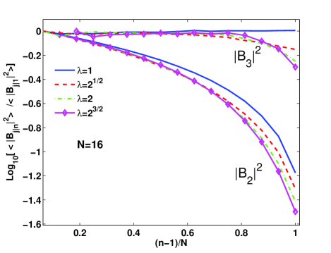
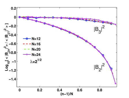
Square amplitude distributions for for different        frequency scaling factor $\lambda=1,\ \sqrt{2},\ 2,\ 2\sqrt{2}$ with        $N=16$. For $\lambda\geq 2$ plots are practically converged.	Square amplitude distributions for different         number of triads $N=16,\ 20,\ 24$ with $\lambda=\sqrt{2}$.        All plots practically coincide
${\mathcal{C}}$	${\mathcal{D}}$
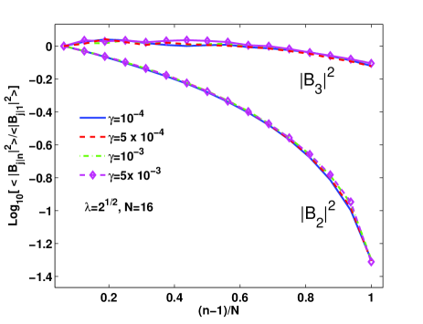
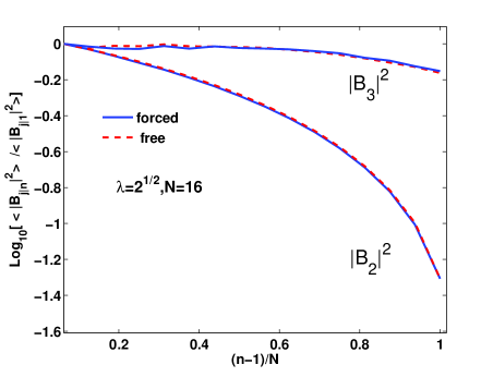
Square amplitude distributions for different $\gamma$         for $\lambda=\sqrt{2}$ and $N=16$.	Comparison of the forced and free chain for $\lambda=\sqrt{2}$        and $N=16$. These two plots practically coincide

Figure 20: Comparison of the plots of $\ln\,\langle|B_{j|n}|^{2}\rangle$ vs $n/(N-1)$ for different $\lambda$, panel ${\mathcal{A}}$, for different $N$, panel ${\mathcal{B}}$ and for different $\gamma$, panel ${\mathcal{C}}$. Panel ${\mathcal{D}}$ compares distributions for the free and forced evolutions.

${\mathcal{A}}$	${\mathcal{B}}$

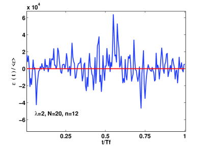
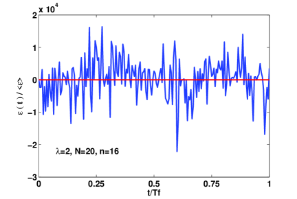
Figure 21: The time evolution of the normalized flux over triad 12 (${\mathcal{A}}$) and over triad 16 (${\mathcal{B}}$) during one period of the forcing triad for $\lambda=2$ for $N=20$.

VI.3.3 Forced- vs free-evolution statistics in the chain clusters

One more surprise is that in the conditions of the energy-flux equilibrium in the scale-invariant situations (in our case, $Z_{n}\propto\lambda^{n}$) we did not observe the expected power-like behavior, when $\langle|B_{j|n}|^{2}\rangle\propto\lambda^{n\,\zeta}$. Moreover, the ratio $\langle|B_{2|n}|^{2}\rangle\big{/}\langle|B_{3|n}|^{2}\rangle$ depends on $n$ and the connected modes $\langle|B_{3|n}|^{2}\rangle$ weakly depend on $n$, as one expects in the thermodynamic equilibrium, after a long free evolution.

That is why we decided to compare forced distributions of $\langle|B_{2|n}|^{2}\rangle$ and $\langle|B_{3|n}|^{2}\rangle$ with the distributions of $\langle|B_{2|n}|^{2}\rangle$ and $\langle|B_{3|n}|^{2}\rangle$ after long free evolutions (without forcing and damping) in the same cluster. For concreteness we took cluster with $\lambda=\sqrt{2}$ and $N=16$ after forced evolution during time $t=1000T_{f}$. To get the values of the forced amplitudes we averaged over last $500T_{f}$. Then we took final complex amplitudes $B_{2|n}$ and $B_{3|n}$ as initial conditions for the free evolution during another period $t=1000T_{f}$, and again averaged over last $500T_{f}$. Both distributions of $\langle|B_{2|n}|^{2}\rangle$ and $\langle|B_{3|n}|^{2}\rangle$ are presented in the Fig. 20$\,{\mathcal{D}}$. As one sees these distributions practicably coincide.

In other words, the distributions with constant energy flux and the distributions with zero energy flux are almost identical. To show, why this happens we presented in Fig. 21 the time evolution of the instant energy flux via $n$-th triad

$$\varepsilon_{n}(t)=2Z_{n}{\rm Re}[{B_{1|n}(t)B_{2|n}(t)B^{*}_{3|n}(t)}]\,,$$ (59)

normalized by its mean value $\widetilde{\varepsilon}_{n}\equiv\langle\varepsilon_{n}(t)\rangle$. One sees enourmous fluctuations of $\varepsilon_{n}(t)$ with peaks, reaching $\approx 6000\,\widetilde{\varepsilon}_{n}$. The computed mean value of the flux fluctuation $\delta\varepsilon_{n}\equiv\sqrt{\langle\varepsilon_{n}^{2}(t)\rangle}$ is about 100 times larger than $\widetilde{\varepsilon}_{n}$. This means that there is a strong energy exchange between triads in the cluster, that essentially exceeds minor mean flux. Therefore one can switch off the mean energy flux without almost any effect on the cluster statistics. We think, that this general statement is valid for all kind on clusters, consisting of connected triads.

The only difference between forced and free long-time evolution of the clusters is the restriction, that follows from the conservations laws, that are satisfied exactly in free evolutions and approximately in the forced case.

VII Conclusions

VII.1 Main points of understanding in finite-dimensional wave turbulence

•  In the first part of the paper we studied the structure of finite clusters of resonant triads using the example of atmospheric planetary waves and showed that:

– In the physically relevant domain of atmospheric planetary waves ($m\,,\ \ell\leq 1000$, when the mode-scale is larger than the height of the Earth atmosphere) we have found and described the topology of all the clusters formed by resonantly interacting planetary modes. The set od clusters contains isolated triads and subsets of 2-, 3-, $\dots$, 16 and 3691 connected triads, with 2- 3-, $\dots$, 9-mode and (maximum) 10-mode connections;

– Analyzing the integrals of motion we suggested a classification i) of triad modes into two types - active (A) and passive (P), and ii) of connection types between triads - AA, AP and PP. We showed explicitly that through the AA-connection the energy can flow in both directions, through the AP-connection only from P-connected triad to the A-connected one, but not vice-versa. The PP-connections are almost impenetrable for energy in both directions. Therefore from the viewpoint of the energy transfer, large clusters can be subdivided into smaller ones (by cutting PP-connections);

– We introduced a notion of PP-irreducible sub-clusters that cannot be further divided by cutting PP-connections and studied their statistics for planetary waves in the spectral domain $m\,,\ \ell\leq 1000$. There are 3005 triads, 400 PA- and AA-butterflies, 143 triple-triad PP-irreducible sub-clusters, etc., and only two 130-triad ones in this domain;

– To first approximation, almost all triads in the methodologically significant domain, Table. 1, can be considered as completely or almost separated from the rest of the atmospheric planetary waves and therefore the energy oscillations between them can really lead to intra-seasonal oscillations in Earth’s atmosphere as suggested in KL-07 .

•  In the second part of the paper we presented a general analysis of the energy transfer in the PP-irreducible sub-clusters. Studying free evolution from asymmetrical initial conditions, when almost all the initial energy is localized in one (leading) triad we showed:

–  the energy flux through the AA- and PA-connections are qualitatively the same and crucially depend on the initial conditions in the leading triad and on the ratio of the interaction coefficients in the leading and driven triads;

–  the energy flux from the leading to two driven triads in triple-triad clusters depends on the type of energy-junction (triple AAA-, PAA-stars or PA-AP chain) and on the relations between three interaction coefficients.

•  We also studied forced stationary energy transfer in a long chain consisting of $N$ PA-connected triads with the interaction coefficients $Z_{n}\propto\lambda^{n}$, $1\leq n\leq N$, with forcing in the first triad and damping in the last one. We showed that stationary energy distributions between triads are universal in the following sense:

–  For $\lambda\geq 1$ the distributions are almost $\lambda$-independent; For $\lambda\geq 2$ the distributions practically collapse on each other.

–  the distributions are practically independent of the damping parameter $\gamma$ for $\gamma<\gamma_{\text{th}}$. For $\gamma>\gamma_{\text{th}}$ the stationary state does not exist.

–  Distributions for the forced case and for the free evolution (with the forced state as initial condition) coincide due to extremely large fluctuations of the energy flux, exceeding its mean value in orders of magnitude.

•  Our analysis of finite-dimensional wave turbulence is based on the simple form (18) of the basic equations and does not exploit the explicit form of the interaction coefficients $Z$ which vary substantially for different wave systems. This means that our results can be used directly for arbitrary 3-wave resonant systems governed by Eqs. (18), e.g. drift waves, gravity-capillary waves, etc.

VII.2 Remaining unclear issues in finite-dimensional and mesoscopic regimes of weak wave turbulence

•  Having in mind the extremely rich variability of the structure of concrete finite clusters of resonance triads and the various important aspects of the cluster dynamics and statistics (some of them were not mentioned at all), this paper opens more questions than answers. Among them:

–  What might be the peculiarities of free evolutions of finite clusters from other initial conditions, more general than those studied in this paper, especially for particular clusters which may be important in some applications?

–  How energy goes through more complicated junctions, than triple stars, studied in this paper, such as stars with four and five and more triads, etc.?

–  How integrability of clusters (with special choice of the ratios of interaction coefficients and/or initial conditions ver ; 08-BK ) or closeness to the integrable cases affect the energy transfer and the statistics of the mode amplitudes?

–  What is the dimensionality of the cluster trajectories, how does it depends on the details of the initial conditions and/or the ratios of interaction coefficients for various cluster structure?

–  How different-mode, different-time correlation functions depend on the mode position in a cluster and on the time difference between them?

–  What is the values of the flatness (ratio of the forth-order correlation functions to the square of the second-order ones) and how does it depend on the cluster structure, initial conditions, etc.?

–  To what extent can the statistics of the amplitudes of individual modes be considered close to Gaussian at least for very large (but finite) clusters?

–  How does this closeness (if it exists) depend on the mode position in a cluster and on initial conditions?

–  If this closeness exists (we believe that it does), how can one formulate appropriate closures that will lead to an analytical statistical description of the finite cluster behavior?

•  A few of the most important questions, at least from the theoretical viewpoint, are:

–  What is the principal difference between finite size cluster behavior for three-wave resonances, discussed here, and that for four-wave resonance systems?

–  How mode statistics and possible applicability of the closure procedures changes, if one accounts for small damping of the mode energy and external random noise, that can mimic interaction of a cluster with the “rest of the world”?

–  How all the features of a cluster behavior (both for those studied and those left open) get modified if one accounts for quasi-resonances that can become crucially important with increasing the level of the modes excitation?

–  How to describe the statistical behavior of finite-size dynamical systems (in the case of three- and four-wave interactions) with further increases in the system size or in the level of system excitation? How this behavior approachs (step by step, probably via an intermediate kind of behavior) the limit of infinite system with quasi-Gaussian statistics, that can be successfully described with the help of wave-kinetic equations?

VII.3 The road ahead

Our feeling is that all these (and many similar and different, but related) questions are the subject of a new fields in nonlinear wave physics, finite-dimensional wave turbulence and mesoscopic wave turbulence. This subject offers very interesting issues both from the physical and the methodological viewpoints, with possible important applications in numerous physical examples.

- (1) V. E. Zakharov, V. S. L’vov, and G. Falkovich, Kolmogorov Spectra of Turbulence (Springer-Verlag, Berlin, 1992)
- (2) Lvov Y, Nazarenko S V, ”Noisy” spectra, long correlations and intermittency in wave turbulence, Physical Review E, 69, 1539-3755 (2004)
- (3) Nazarenko S V, Choi Y, Lvov Y, Joint statistics of amplitudes and phases in Wave Turbulence, Physica D: Nonlinear Phenomena, 201, 121-149 (2005).
- (4) Yuri V. Lvov, Sergey Nazarenko, Boris Pokorni, Discreteness and its effect on water-wave turbulence, Physica D: Nonlinear Phenomena 218, 24-35 (2006)
- (5) A.C. Newell, V.E. Zakharov, The role of the generalized Phillips’ spectrum in wave turbulence, Physics Letters A 372, 4230-4233 (2008)
- (6) E. Kartashova, V.S. L’vov. Phys. Rev. Lett. 98, 198501 (2007)
- (7) E. Kartashova and V.S. L’vov, Europhys. Letters 83, 50012 (2008).
- (8) V. I. Arnold, Geometrical Methods In The Theory Of Ordinary Differential Equations, Springer-Verlag (1988).
- (9) E. Kartashova, JETP Lett., 83, 341 (2006).
- (10) S. Nazarenko, 2D enslaving of MHD turbulence, New J. Phys. 9 307 (2007).
- (11) V. E. Zakharov, A. O. Korotkevich, A. N. Pushkarev and A. I. Dyachenko, Mesoscopic wave turbulence, JETP Letters 82(8), 487-491 (2006)
- (12) J. Pedlosky, Geophysical Fluid Dynamics, (Second edition, Springer-Verlag, 1987)
- (13) Jacobs et al., Nature 370, 360 (4th August 1994)
- (14) F. Isotta et al., Int. J. Climatol. (2008)
- (15) E. Kartashova, A. Kartashov., Physics A: Stat. Mech. Appl. 380, 66 (2007)
- (16) E. Kartashova, C. Raab, Ch. Feurer, G. Mayrhofer, W. Schreiner, In: Extreme Waves in the Oceans, eds.: Ch. Harif and E. Pelinovsky, Springer (to appear). E-print: arXiv:0706.3789v2 [nlin.PS] (2008)
- (17) Zakharov V.E. et al., JETP Letters 82, 491 (2005)
- (18) M. Tanaka, J. Phys. Oceanogr. 37, 1022 (2007)
- (19) P. Denissenko, S. Lukaschuk, S. Nazarenko, Phys. Rev. Lett. 99, 014501 (2007)
- (20) Isadore Siberman, Planetary waves in the Atmosphere, J. Atm. Sci. 11, 27-34 (1954).
- (21) M. Ghil, D. Kondrashov, F. Lott, and A.W. Robertson, Pis’ma Zh. Eksp. Teor. Fiz. 82, 544 (2005); see also an extensive bibliography therein.
- (22) K. Hasselmann, J. Fluid Mech., 30, 737 (1967).
- (23) E. Kartashova, private communication, 2007.
- (24) L. F. Shampine, and M. W. Reichelt, SIAM Journal on Scientific Computing, 18, 1, (1997).
- (25) F. Verheest, J. Phys. A: Math. Gen., 21, L545 (1988); J. Math. Phys., 29 2197 (1988)
- (26) M.D. Bustamante and E. Kartashova, EPL, 85, 14004 (2009).
- (27) V.S. L’vov and I. Procaccia. Exact Resummation in the Theory of Hydrodynamic Turbulence. 0. Line-Resummed Diagrammatic Perturbation Approach. Lecture Notes of the Les Houches 1994 Summer School “Fluctuating Geometries in Statistical Mechanics and Field Theory”, ed. by F. David and P. Ginsparg North-Holland, Amsterdam, pp. 1027 - 1075 (1995)
- (28) Uriel Frisch, Turbulence: The Legacy of A. N. Kolmogorov (Cambridge University Press, Cambridge, England, 1995)