Synchronization in non dissipative optical lattices

Abstract

The dynamics of cold atoms in conservative optical lattices obviously depends on the geometry of the lattice. But very similar lattices may lead to deeply different dynamics. In a 2D optical lattice with a square mesh, it is expected that the coupling between the degrees of freedom leads to chaotic motions. However, in somme conditions, chaos remains marginal. The aim of this paper is to understand the dynamical mechanisms inhibiting the appearance of chaos in such a case. As the quantum dynamics of a system is defined as a function of its classical dynamics – e.g. quantum chaos is defined as the quantum regime of a system whose classical dynamics is chaotic – we focus here on the dynamical regimes of classical atoms inside a well. We show that when chaos is inhibited, the motions in the two directions of space are frequency locked in most of the phase space, for most of the parameters of the lattice and atoms. This synchronization, not as strict as that of a dissipative system, is nevertheless a mechanism powerful enough to explain that chaos cannot appear in such conditions.

1 Introduction

Optical lattices are one of the most efficient tools to manipulate cold atoms, by tuning or adjusting parameters such as the mesh and height of the sites (atom confinement, atomic density), or the lattice geometry. Thus it is not surprising that they became a toy model in many fields. However, depending on the considered situation, the role of the interactions between atoms varies a lot. Condensed matter systems and strongly correlated cold atoms in optical lattices offer deep similarities. The flexibility of the latter allowed the observation of the superfluid-Mott insulator quantum phase transition mott , of the Tonks-Girardeau regime tonks , and more generally to the superfluidity properties, including the instabilities. In these experiments, the interactions between the cold atoms play a major role, and require the use of a Bose-Einstein condensate. In particular, instabilities are described by the Gross-Pitaevskii equation, through the non-linear term kuan . Quantum computing also required a coupling between qubits. Optical lattices with controlled or “on demand” interactions appear to be an efficient implementation of a Feynman’s universal quantum simulator quantum simulator , and are among the most promising candidates for the realization of a quantum computer mandel2004 .

On the other hand, interesting behaviors can be found in noninteracting systems. In many situations, including the one considered here, the underlying physics is that of a single atom, without any interaction between neighbors. The higher number of atoms simply increases the observable signal. It is the case in statistical physics, where cold atoms in optical lattices, through their tunability, made possible the observation of the transition between Gaussian and power-law tail distributions, in particular the Tsallis distributions tsallis ; anders . Non-interacting cold atoms in optical lattices also allowed the observation of Anderson localization anderson aspect ; anderson roati ; anderson garreau . Such cold atoms appear also to be an ideal model system to study the dynamics in the classical and quantum limits. Both are closely related, as the latter is only defined as a function of the former. For example, quantum chaos is defined as the quantum regime of a system whose classical dynamics is chaotic. A good understanding of the classical dynamics is therefore an essential prerequisite to the study of quantum dynamics. In non dissipative optical lattices, both the classical and the quantum situations are experimentally accessible, and it is even possible to change quasi continuously from a regime to the other raizen2000 . Moreover, the extreme flexibility of the optical lattices makes it possible to imagine a practically infinite number of configurations by varying the complexity of the lattice and the degree of coupling between the atoms and the lattice. Many results have been obtained during these last years in the field of quantum chaos raizen2000 ; lignier2005 . As mentioned above, these results in the quantum regime follow extensive studies of the classical system CKR .

Most of the above works used very simple potentials, mainly 1D. For example, chaos is obtained only with a periodic (or quasi-periodic) temporal forcing of the amplitude or frequency of the lattice raizen2000 ; lignier2005 , and only the temporal dynamics of the individual atoms is studied. But recently, it appeared necessary to introduce more complex potentials, in particular 2D potentials guo2009 . Although the dynamics of particles in 2D potential has been extensively studied in the past, it was mainly in model potentials chaikovsky1991 ; panoiu2000 . Experimental optical lattices approach these models at best on a limited domain, at the bottom of the wells. But in most cases, the potential is more complex, and leads to a more complex and richer dynamics philo . Understanding acutely the classical dynamics of atoms in real potentials is important, in particular because it has significant consequences in the corresponding quantum systems.

The most common approach for the study of complex dynamics in conservative systems is statistical, e.g. evaluating the percentage of the chaotic area in the phase space. However, a more deterministic approach is possible, as in dissipative systems. In a recent study, we studied the dynamics of atoms in different 2D conservative optical lattices. We chose experimentally feasible lattices, as these studies were motivated by experiments, and we showed that different types of chaotic dynamics appear, leading to different macroscopic behaviors: we showed in particular that the lifetime of atoms in the lattices depend drastically on their dynamics philo .

One of the simplest experimental 2D conservative potential that we studied in philo is the square lattice, resulting from the interference of 2 orthogonal pairs of counter-propagating stationary waves. This lattice has a square mesh, and the two directions in space are strongly coupled. Therefore the dynamics is expected to be fully chaotic when anharmonicity is high enough, i.e. for high enough energy of the atoms. This fully chaotic regime is effectively observed, except when the lattice is red detuned. In this case, chaos disappeared almost completely, and the dynamics remains essentially quasiperiodic, although the nonlinearities remain the same. The reasons of this unusual behavior was not discussed inphilo , where we focused on the chaotic behaviors. However, the lack of chaos where it is expected deserves to be studied in details, to understand what are the mechanisms inhibiting its appearance?

In the present paper, we give some answers to this question by studying in detail the square optical lattice with red detunings. We show that at the bottom of the wells, the resonance frequencies in both directions are degenerate, but when the atom energy increases, this degeneracy should obviously disappear because of the anharmonicity of the potential. However, we show that the motions in both directions remain locked to the same frequency on a large domain, following a synchronization mechanism close to the frequency locking process of dissipative systems. Because of the conservation of energy, it is not a strict frequency locking, but the quasiperiodic regime appears to be mainly a frequency locked periodic regime with small sidebands. Even when the edges of the wells are approached, chaos appears very marginally, in a regime where the frequencies remain locked. The paper is organized as follows: after this introduction, we discuss the model of the lattice, and we search analytically for periodic solutions at the bottom of the well, where approximations lead to a Duffing-like model. Then we discuss the general case, i.e. far from the bottom of the well. In this case, results are obtained mainly from numerical simulations. We show that the main frequency of the motion is the same in both directions, whatever the energy is, and we analyze the mechanisms leading to this synchronization.

2 Description of the square lattice

When cold atoms are dropped in a stationary wave, they undergo a force $F$, the potential $U$ of which is proportional to the wave intensity $I$, and inversely proportional to the detuning $\Delta$ between the wave frequency and the atomic transition frequency:

$$F = -\nabla U$$

$$U \propto \frac{I}{\Delta}$$

The detuning is a key parameter for the behavior of the atoms: they accumulate in bright sites for red detunings ($\Delta<0$), and in dark sites for blue detunings ($\Delta>0$). This paper is restricted to the red detuned case, i.e. atoms located in the bright areas. When the atoms are cooled with a Magneto Optical Trap (MOT), the atomic density in these optical lattices is small enough to neglect the collisions between atoms, and so the only source of dissipation is the spontaneous emission. As spontaneous emission is proportional to $I/\Delta^{2}$, it is relatively easy to build conservative optical lattices.

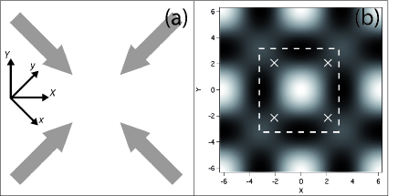
Figure 1: a) Layout of the laser beams. b) Spatial distribution of the intensity in the $\left(X,Y\right)$ space for $\alpha=0.5$. Black corresponds to the minimum value (zero intensity), while white corresponds to the maximum. The dashed square delimits the elementary mesh of the lattice, and the white crosses are the saddle points.

The lattice geometry is a decisive parameter for the motion of the atoms. Many geometries can be experimentally built, as a vertical stack of ring traps courtade2006 , five-fold symmetric lattice guidoni1999 or quasiperiodic lattices guidoni1997 . But one of the simplest experimental optical lattice is the case of two orthogonal stationary plane waves with the same linear polarization. The configuration of the laser beams is shown on Fig. 1a. The total field is $\mathcal{E}=\cos kx+e^{i\phi}\sin ky$, where $x$ and $y$ are the two space coordinates, $\phi$ a phase, $k=2\pi/\lambda$ the wave vector and $\lambda$ the wavelength of the laser beam. The intensity can be written as:

$$I=\cos^{2}kx+\cos^{2}ky+2\alpha\cos kx\cos ky$$

where $\alpha=\cos\phi$. With the adequate normalization, the potential is, for $\Delta<0$:

$$U=-I$$

When $\alpha=0$, the coupling between $x$ and $y$ disappears, and the problem becomes separable. In all the other cases, the coupling between $x$ and $y$ could induce complex dynamics. It is easy to see that in these cases the elementary mesh of the potential is turned of $\pi/4$ as compared to the $\left(x,y\right)$ axes, and thus it is natural to introduce the following new coordinates:

$$X = kx+ky$$

$$Y = ky-kx$$

The intensity and the potential can now be written:

$$I=-U=1+\alpha\left(\cos X+\cos Y\right)+\cos X\cos Y$$ (1)

The minus sign is that of the red detuning ($\Delta<0$) that we consider here. In this conditions, the atoms accumulate in the bright areas: the maxima of intensity correspond to the minima of the potential. For blue detunings, atoms accumulate in the dark areas, leading to significant differences in the motion philo .

As an example, the following of the paper will be illustrated with numerical values and plots obtained with $\alpha=0.5$. The choice of this value is not restrictive, and these illustrations are representative of the behaviors for other values of $\alpha$. Fig. 1b shows the spatial distribution of the intensity in this case. The elementary mesh is indicated through the dashed line. Assuming $\alpha>0$, the potential $U$ has its main well at the absolute minimum $E_{0}=-2\left(1+\alpha\right)$ at coordinates $\left(n2\pi,m2\pi\right)$, where $m$ and $n$ are integers. It has also a relative minimum $-2\left(1-\alpha\right)$ in $\left(\pi+n2\pi,\pi+m2\pi\right)$. $\alpha=0$ is a special case because the absolute and relative minima have the same value. The intensity goes to zero in $\left(\pi+n2\pi,m2\pi\right)$ and $\left(n2\pi,\pi+m2\pi\right)$, corresponding to the maxima of the potential. Two neighboring maxima are separated by a saddle point where $U=E_{T}=-\left(1-\alpha^{2}\right)$ (remind that $\alpha\leq 1$). $E_{T}$ is the minimum energy required for a classical atom to jump from one well to another one. In the quantum world, atoms can also tunnel through the barrier, leading to a band structure. However, we do not have to consider the tunnelling here, because, prior to any quantum treatment, the classical behavior has to be deeply understood. On the other hand, it has been shown that, for wells deep enough, the tunnelling vanishes bloch . Thus atoms, the energy $E$ of which is smaller than the threshold $E_{T}$, are trapped into one site. On the contrary, atoms with $E>E_{T}$ can travel between sites, if they move in the right direction. It is also important to note that these saddle points are on the bissectors, connecting on a straight line a main well to a secondary one and again to the next main well. Thus an atom with $E>E_{T}$ following this straight line does not meet any obstacle: bissectors are clearly escape lines.

Inside a trap site, the energy of the atom plays the role of a stochastic parameter. Indeed, for low energies, the atoms remain located close to the bottom of the well, and their dynamics can be approximated by an harmonic motion. As the energy increases, the potential becomes more and more anharmonic, the nonlinearities increase, and the dynamics can become more and more complex philo .

3 The lattice around the origin: periodic solutions

We study in the following the classical dynamics of cold atoms in an optical lattice, and more generally that of a classical particle in the corresponding potential. Let us first examine what is the motion at the bottom of a main well. We approximate the potential to the fourth order:

$$U=-\left(\alpha+1\right)\left(D_{X}+D_{Y}\right)-\frac{X^{2}Y^{2}}{4}$$ (2)

with

$$D_{X} = 1-\frac{X^{2}}{2}+\frac{X^{4}}{24}$$

$$D_{Y} = 1-\frac{Y^{2}}{2}+\frac{Y^{4}}{24}$$

$D_{X}$ and $D_{Y}$ have the shape of the potential of a conservative Duffing oscillator. Thus the motion of the particles at the bottom of a well appears to follow the dynamics of two coupled Duffing oscillator, and so we can search for approximate harmonic solutions. The equations to solve are immediately derived from eq. (2):

$$F_{X} = -\left(\alpha+1\right)\left(X-\frac{X^{3}}{6}\right)+\frac{XY^{2}}{2}$$ (3a)

$$= \ddot{X}$$ (3b)

$$F_{Y} = -\left(\alpha+1\right)\left(Y-\frac{Y^{3}}{6}\right)+\frac{X^{2}Y}{2}$$ (3c)

$$= \ddot{Y}$$ (3d)

Let us first search if periodic oscillations are approximate solutions of these equations. We search for:

$$X = X_{0}\cos\left(\omega t+\psi_{X}\right)$$ (4a)

$$Y = Y_{0}\cos\left(\omega t+\psi_{Y}\right)$$ (4b)

where $X_{0}$, $Y_{0}$, $\omega$, $\psi_{X}$ and $\psi_{Y}$ are constant. First, we look at the constraints that have to be satisfied for the solutions. Then, to fully characterize a solution, we need to check its stability, i.e. the behavior of the trajectories close to that solution. In a dissipative system, a stable periodic orbit is an attractor, and thus it plays a crucial role in the effective dynamics of the system. On the contrary, an unstable periodic orbit is not directly observable in experiments. The situation is not so different in a conservative system. A periodic orbit is stable if the behavior in its vicinity changes slowly with the distance, i.e. if the trajectories change continuously from the periodic orbit to a torus. The motion in the vicinity of the periodic orbit is then not very different from a periodic oscillation. On the contrary, if the periodic orbit is unstable, a small change in the initial conditions leads to a completely different behavior, which cannot be considered as a small perturbation of the initial periodic cycle.

The force terms in (3) are developed in their Fourier components, dropping the higher harmonics:

$$F_{X} = A_{X}\cos\left(\omega t+\psi_{X}\right)+B_{X}\sin\left(\omega t+\psi_{X}\right)$$ (5a)

$$F_{Y} = A_{Y}\cos\left(\omega t+\psi_{Y}\right)+B_{Y}\sin\left(\omega t+\psi_{Y}\right)$$ (5b)

$A_{X,Y}$ and $B_{X,Y}$ are the corresponding Fourier components:

$$A_{X,Y} = \frac{\omega}{\pi}\int_{0}^{2\pi/\omega}dt\,F_{X,Y\,}\cos\left(\omega t+\psi_{X,Y}\right)$$ (6a)

$$B_{X,Y} = \frac{\omega}{\pi}\int_{0}^{2\pi/\omega}dt\,F_{X,Y\,}\sin\left(\omega t+\psi_{X,Y}\right)$$ (6b)

which lead to:

$$A_{X} = -X_{0}\left(1+\alpha\right)+\frac{X_{0}^{3}}{8}\left(1+\alpha\right)$$ (7a)

$$+\frac{X_{0}Y_{0}^{2}}{8}\left(2+\cos\left(2\psi_{Y}-2\psi_{X}\right)\right)$$

$$B_{X} = -\frac{X_{0}Y_{0}^{2}}{8}\sin\left(2\psi_{Y}-2\psi_{X}\right)$$ (7b)

$$A_{Y} = -Y_{0}\left(1+\alpha\right)+\frac{Y_{0}^{3}}{8}\left(1+\alpha\right)$$ (7c)

$$+\frac{X_{0}^{2}Y_{0}}{8}\left(2+\cos\left(2\psi_{Y}-2\psi_{X}\right)\right)$$

$$B_{Y} = -\frac{X_{0}^{2}Y_{0}}{8}\sin\left(2\psi_{Y}-2\psi_{X}\right)$$ (7d)

Differentiating twice the equations (4), we obtain another expression for the system equations which imposes $B_{X}=B_{Y}=0.$ There are 6 periodic solutions for Eqs (3):

$$X_{0} = 0$$ (8a)

$$Y_{0} = 0$$ (8b)

$$\psi_{X} = \psi_{Y}$$ (8c)

$$\psi_{X} = \psi_{Y}+\pi$$ (8d)

$$\psi_{X} = \psi_{Y}-\frac{\pi}{2}$$ (8e)

$$\psi_{X} = \psi_{Y}+\frac{\pi}{2}$$ (8f)

The trivial solutions (8a) and (8b) are those of a particle oscillating along one of the main directions, where the minimum of the motion coincides with the bottom of the well. As the potential is invariant when $X$ and $Y$ are exchanged, we have to study only one of these solutions. The antiphase solution (8d) corresponds to a change of sign of $Y$ as compared to in-phase solution (8c). As the potential is even in $X$ and $Y$, we need to study only one of them. For the same reasons, only one of the quadrature solutions (8e) and (8f) has to be studied.

Trivial solutions

Let us first look at the $Y_{0}=0$ trivial solution. It comes immediately from Eqs (7a) and (3) that the frequency of the motion is:

$$\omega^{2}=\omega_{0}^{2}\,\left(1-\frac{X_{0}^{2}}{8}\right)$$ (9)

where $\omega_{0}=\sqrt{1+\alpha}$ is the frequency of the oscillations at the very bottom of the wells. This relation is nothing but the well-known dependence on the amplitude of motion, of the period of oscillation for a simple pendulum $T=T_{0}\,\left(1+\frac{X_{0}^{2}}{16}\right)$.

Let us look in the neighboring of our trivial solution. For $Y$ small, Eq. (3c) writes:

$$\ddot{Y}+\omega_{0}^{2}\,Y-\frac{X^{2}Y}{2}=0$$ (10)

With a solution of the type of (4a), this equation becomes

$$\ddot{Y}+\left(\omega^{2}-\frac{X_{0}^{2}}{8}\left(1-\alpha\right)-\frac{X_{0}^{2}}{4}\,\cos 2\omega t\right)Y=0$$ (11)

This equation is that of a parametric oscillator with a frequency close to $\omega$, with no damping, and excited at the frequency $2\omega$. Such an oscillator is known to diverge rapidly, and thus the behavior in the vicinity of the trivial solutions does not remain close to these solutions. Thus trivial solutions are unstable solutions of the system.

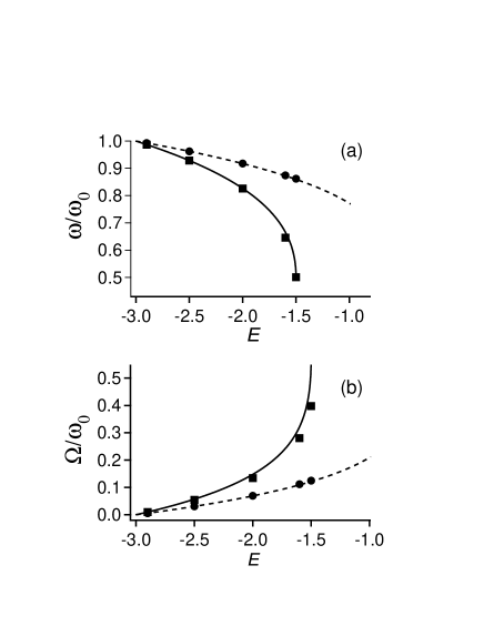
Figure 2: Oscillation frequencies of the particle in the vicinity of the periodic orbits, in the case of the Duffing approximation. In (a), frequency of the periodic solution; in (b), frequency of the beating. The solid (resp. dashed) lines refer to the analytical in-phase (resp. quadrature) frequencies. The square (resp. round) markers refer to the values computed through numerical simulations, of the in-phase (resp. quadrature) solutions.

In-phase and antiphase solutions

Let us now look at the (8c) in-phase solution. Eqs (7a) and (7c) give two expressions for $\omega$, which are compatible only if the motions in the two directions have the same amplitude $X_{0}^{2}=Y_{0}^{2}$, with a frequency given by:

$$\omega_{1}^{2} = \omega_{0}^{2}-\left(1+\frac{\alpha}{4}\right)\frac{X_{0}^{2}}{2}$$ (12)

This solution appears to be very similar to the trivial solutions: the particles oscillate along a straight line, namely one of the bissectors. Their frequency decreases as the motion amplitude increases. However, as the stochastic parameter of our potential is the energy, it is more convenient to represent the evolution of the dynamics as a function of this parameter. The conversion between amplitude and energy depends on the motion. For the present motion, the total energy $E_{1}$ leading to a motion amplitude of $X_{0}$ is equal to the potential energy in $\left(X_{0},X_{0}\right)$. Thus the relation between $X_{0}$ and $E_{1}$ is easily deduced from Eq. (2):

$$E_{1} = \omega_{0}^{2}\,\left(X_{0}^{2}-2\right)-\left(\alpha+4\right)\frac{X_{0}^{4}}{12}$$ (13)

Fig. 2a shows (solid line) the evolution of $\omega_{1}$ as a function of the energy, for $\alpha=0.5$. In this case, the bottom of the main well corresponds to an energy $E_{0}=-3$, while the saddle in the full model corresponds to $E_{T}=-0.75$. The Duffing model is an approximation of the motion at the bottom of well, i.e. for energies of the order of $E_{0}$. For higher energies, the Duffing approximation diverges from the full model. In particular, the threshold energy in the Duffing approximation is $E_{D}=-1.5$, and the in-phase solution vanishes for larger energies, as shown in Fig. 2a. The reason is that the motion occurs exactly along the bissector, where is also located the threshold between the wells. When the threshold energy is reached, the particle leaves the well.

To estimate more precisely the domain of validity of the Duffing approximation, it is more intuitive to use the motion amplitude rather than the energy. Eq. (13) gives the relation between $E$ and $X_{0}$ for the (8c) and (8d) solutions: one finds that $X_{0}=1$ corresponds to $E=-1.875$, which corresponds to the half height of the non-approximated well. This means that the interval on which the Duffing approximation is realistic is typically $-3<E\lesssim-1.875$.

To evaluate the stability of this solution, we study the motion in its vicinity. We search for solutions of the type:

$$X = \left(X_{0}+\varepsilon_{X}\right)\cos\left(\omega_{1}t+\phi_{X}\right)$$

$$Y = \left(X_{0}+\varepsilon_{Y}\right)\cos\left(\omega_{1}t+\phi_{Y}\right)$$

If this solution is injected into the motion equations, one finds that $\varepsilon_{X}+\varepsilon_{Y}=C$ where $C$ is a constant. It is easy to show that taking $C\neq 0$ is equivalent to translate from the solution $\left(X_{0},X_{0}\right)$ to the solution $\left(X_{0}+\frac{C}{2},X_{0}+\frac{C}{2}\right)$. Thus we choose $\varepsilon_{X}=-\varepsilon_{Y}=\varepsilon$. The equations of motion, in the slow varying envelop approximation (SVEA), become:

$$\dot{\phi}_{X}-\dot{\phi}_{Y} = \left(1-\frac{\alpha}{2}\right)\frac{X_{0}}{2\omega_{1}}\varepsilon$$ (14a)

$$\dot{\varepsilon} = -\frac{X_{0}^{3}}{8\omega_{1}}\left(\phi_{X}-\phi_{Y}\right)$$ (14b)

or:

$$\ddot{\varepsilon}+\Omega_{1}^{2}\varepsilon = 0$$

with

$$\Omega_{1} = \frac{X_{0}^{2}}{4\omega_{1}}\sqrt{1-\frac{\alpha}{2}}$$ (15)

The perturbation of the in-phase solution oscillates, and thus the in-phase solution is a stable periodic orbit. The amplitudes of the motions along $X$ and $Y$ are modulated in antiphase at the frequency $\Omega_{1}$. A phase modulation, in quadrature with the amplitude modulation, is also present, as expressed in (14b). The neighboring solutions are quasiperiodic solutions with the same main frequency $\omega_{1}$, and sidebands at the frequency $\Omega_{1}$ increasing with the energy (Fig. 2b, solid line). Note that for the highest energies ($E=-1.5$), $\Omega_{1}\simeq\omega_{1}$, and thus the SVEA is no more valid. However, we already established above that this energy domain is not fully relevant, as the Duffing approximation is itself too much rough to describe the experimental system for such energies. Thus the valid domain remains typically $-3<E\lesssim-1.875$, as discussed previously.

As argued above, the $\psi_{X}=\psi_{Y}+\pi$ solution is the same solution as $\psi_{X}=\psi_{Y}$ when $Y$ is changed in $-Y$. It consists in a particle oscillating on the other bissector. This solution $\left(X_{0},-X_{0}\right)$ is stable, and neighboring solutions are an oscillating motion around the main solution. The dependence between the frequencies and the energy is the same as in the $\psi_{X}=\psi_{Y}$ solution.

Quadrature solutions

The last pair of solutions are those where $X$ and $Y$ oscillate in quadrature of phase. The same steps as for the $\psi_{X}=\psi_{Y}$ lead to the solutions:

$$X = X_{0}\cos\left(\omega_{2}t\right)$$ (16a)

$$Y = X_{0}\cos\left(\omega_{2}t\pm\frac{\pi}{2}\right)$$ (16b)

with:

$$\omega_{2}^{2} = \omega_{0}^{2}-\left(2+\alpha\right)\frac{X_{0}^{2}}{8}$$ (17)

The motion of a particle is a circle around the origin. The only difference between both solutions is the rotation direction. The analysis of the motion in the neighboring of these solutions leads to an oscillating motion with a frequency:

$$\Omega_{2} = \frac{X_{0}^{2}}{4\omega_{2}}\sqrt{\frac{\alpha}{2}}$$ (18)

These solutions are stable periodic orbits, and the motion in the neighboring is quasiperiodic, with a main frequency $\omega_{2}$ decreasing with the energy, and sidebands at a frequency $\Omega_{2}$ increasing with the energy (Fig. 2, dashed lines). Note that for a circular motion, the kinetic energy never vanishes: this is why this motion still exists for total energies larger than $-1.5$, as it does not reach the saddle point.

To summarize the above results, we found that the dynamics in the bottom of the main well of the lattice is organized around two unstable periodic orbits and four stable periodic orbits. As expected, the dynamics in the vicinity of these stable periodic orbits follows KAM tori. These quasiperiodic regimes can be described as a motion at the same frequency as the periodic orbits, perturbed by sideband components. Although this system consists in two perturbed pendula, the effects of the small perturbation is outstanding: whereas uncoupled pendula can oscillate with any relative phase, the coupling introduced here allows only four relative phases, even for very small motions, where the perturbation tends to zero. To evaluate the pertinence of the above description, let us now switch to the results of numerical simulations.

4 Numerical simulations in the Duffing approximation

The aim of numerical simulations is to determine how the previous results evolve far from the bottom of the potential wells. Let us first examine the results of numerical simulations in the Duffing approximation. The interest of such simulations is to give complementary information as compared to the previous results, as the shape of the $X$ and $Y$ time evolution, or the complexity of the spectra.

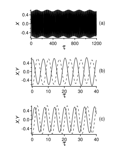
Figure 3: Motion of the particles as a function of the time $\tau=\omega_{0}t$, for $\alpha=0.5$ and $E=-2.5$. (a) large scale motion along $X$; (b) oscillations along $X$ (solid line) and $Y$ (dashed line) in the vicinity of the antiphase solution; (c) oscillations along $X$ (solid line) and $Y$ (dashed line) in the vicinity of a quadrature solution.

Fig. 3 shows the time evolution of $X$ and $Y$ in the vicinity of the antiphase solution (Fig. 3b) and of one of the quadrature solution (Fig. 3c) for $\alpha=0.5$ and $E=-2.5$. In first approximation, it seems that the time evolution in both directions follows the same frequency, with a clear phase relation between them. However, the small amplitude modulation (Fig. 3a) shows that other frequencies are present.

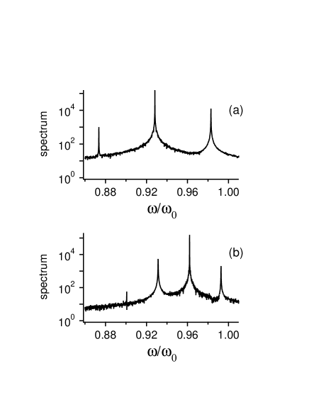
Figure 4: Spectrum of the motion of the particles along the $X$ direction, in the vicinity of the (a) anti-phase solution, and (b) quadrature solution. These are respectively the FFT of the signals of Figs 3b and 3c. Both spectra are represented with the same scales, to make the comparison easier.

More details can be found on the Fourier transform of the signals (Fig. 4). Both dynamics appear to be driven by a main frequency shifted as compared to the frequency $\omega_{0}=\sqrt{1+\alpha}$ at the bottom of the well. The sidebands are more than one order of magnitude weaker, and the second sidebands are still two orders of magnitude smaller. Thus the dynamical regimes along the $X$ and $Y$ directions can effectively be approximated as two frequency locked oscillations, slightly perturbed by a sideband modulation.

It can be noticed that the spectra of Fig. 4 are asymmetric. On Fig. 4a, the high frequency sideband is larger than the low frequency one, while it is inverted on Fig. 4b. This sideband imbalance is simply due to the fact that we have both amplitude modulation and phase modulation. The coupling between these two modulations, expressed in (14a) and (14b) for the in-phase solution, leads to a high frequency component stronger than the low frequency one, as observed in Fig. 4a. On the contrary, for the quadrature solutions, the high frequency sideband is predicted to be weaker than the low frequency one.

The frequencies obtained by the simulations are reported on Fig. 2. For low energies, they are identical to those predicted theoretically in the previous section. For higher energies, small differences appear, in particular for the sidebands of the antiphase solution. This originates, as discussed previously, from the fact that the SVEA is no more valid in this domain, as $\omega_{1}\simeq\Omega_{1}$.

5 Behaviors far from the bottom of the wells

In the above sections, the approximation of the optical lattice to two coupled Duffing oscillators allows us to show that in the vicinity of the bottom of the well, the dynamics is governed by a synchronization process, very similar to the frequency locking. It is well known that this type of phenomenon is able to inhibit complex dynamics in dissipative systems, and if this synchronization applies to a large part of the well, it could explain that chaos appears only into a very narrow area. We study in this section the dynamics of the particles beyond the domain where the Duffing approximation is valid.

Before to examine in details the dynamics of the particles in the exact potential, let us remind the global evolution of the dynamics in the Poincaré section. Our phase space is 4-dimensional, with directions $\left(X,Y,\dot{X},\dot{Y}\right)$, but because of the energy conservation, the accessible space reduces to a 3D surface. We choose to consider Poincaré section at $\dot{Y}=0$ with increasing values, and thus, Poincaré sections are in the 3D space $\left(X,Y,\dot{X}\right)$, and they lie on a 2D surface $S_{P}$, which has the shape looking like a semi-ellipsoid. To represent the Poincaré sections we could project them on the $\left(X,Y\right)$ plane, but we use here the more usual $\left(X,\dot{X}\right)$ plane. It shows the Poincaré sections viewed from the vertex of the semi-ellipsoid. However , because of the stiff sides of $S_{P}$, we have to keep in mind that many curves are projected almost at the same location, and thus are superimposed.

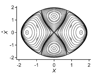
Figure 5: Poincaré sections for $\alpha=0.5$ and $E=-1.02$.

For relatively high energies, we know that the Duffing approximation is no more valid. Thus it is interesting to look if, in spite of that, the behaviors remain those described in the Duffing approximation. As an example, we choose arbitrarily to illustrate the following of the paper with the behaviors obtained for $E=-1.02$, i.e. an energy well above the domain of validity of the Duffing approximation. These behaviors are representative to those observed for all large energy values, i.e. typically larger than $-2$. Fig. 5 shows the Poincaré section in this situation. These results have been obtained through numerical resolution of the equations of motion which are derived from the potential (1), without any approximation. We see four distinct domains separated by an X-shaped separatrix. The central point $\left(X=0,\dot{X}=0\right)$ corresponds to the first trivial solution (8a). This solution has been found to be unstable, which is compatible with the fact that all trajectories move away from it. The second unstable periodic orbit corresponds to $Y=0$, and so $\dot{Y}=0$, and thus it cannot be represented in this Poincaré section through the $\dot{Y}=0$ plane.

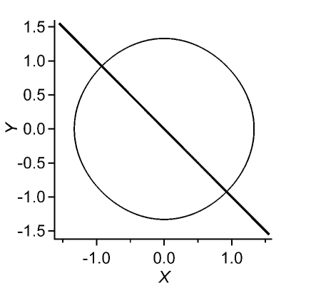
Figure 6: Real space trajectories for the antiphase and the quadrature solutions, calculated for $\alpha=0.5$, $E=-1.02$. The antiphase solution consists in an oscillation of the particle along the straight line, while the quadrature solutions correspond to a rotation of the particle along the circle.

In the right and left domains, the Poincaré sections are closed curves around two points with $\dot{X}=0$. As by definition of the Poincaré section, $\dot{Y}=0$, these points are turning points of the motion, and thus correspond to the in-phase and antiphase solutions. In the same way, in the top and bottom domains, the trajectories are also cycling around two points, with $X=0$, which correspond to the quadrature solutions. Fig. 6 shows the real space trajectories of the antiphase solution and of one of the quadrature solutions. The antiphase solution appears as a straight line on a bissector, along which the particle oscillates with the frequency $\omega^{\prime}_{1}$. The quadrature solution appears as a circle around which the particle turns with the frequency $\omega^{\prime}_{2}$. The values of $\omega^{\prime}_{1}$ and $\omega^{\prime}_{2}$ are reported on Fig. 7a as a function of the energy. As expected, the values predicted with the Duffing approximation and those obtained from the full model diverge significantly for energies larger than -2. However, the global evolution remains that the main frequency decreases as energy is increased.

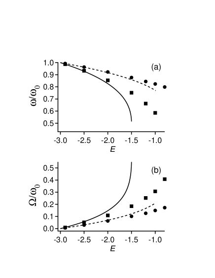
Figure 7: Oscillation frequencies of the particle in the vicinity of the periodic orbits. In (a), frequency of the periodic solution; in (b), frequency of the beating. The solid (resp. dashed) lines are the same as in Fig. 2, i.e. they refer to the analytical in phase (resp. in quadrature) frequencies in the Duffing approximation. The square (resp. round) markers refer to the values computed, through numerical simulations of the full model, for the in-phase (resp. in-quadrature) solutions.

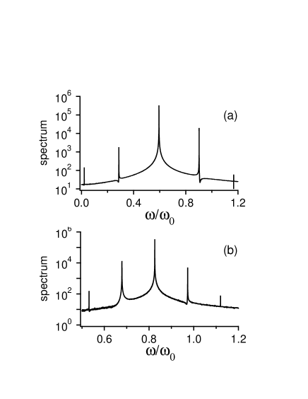
Figure 8: Spectrum of the motion along the $X$ direction, in the vicinity of the (a) antiphase solution, and (b) quadrature solution for $\alpha=0.5$, $E=-1.02$. The corresponding trajectories give the Poincaré sections which are the first circles around the periodic solutions in Fig. 5. In (a), Poincaré section crossing the $\dot{X}=0$ axis in $X=1.46$. In (b), Poincaré section crossing the $X=0$ axis in $\dot{X}=1.195$.

Let us now examine the dynamics on the tori close to a periodic stable solution. We know that for lower energies, it can be considered as periodic oscillations slightly perturbed by sidebands. To know if this approximation is still valid for larger energies, we look at the spectra of the trajectories. Fig. 8 shows the spectrum of two trajectories close to the antiphase and quadrature solutions. The spectra have definitely the same characteristics as those found for the lowest energies: the dynamics is mainly a periodic oscillation, with the same frequency in both directions. This oscillation is perturbed by sidebands, the amplitude of which is more than one order of magnitude smaller. The second sideband is still one order of magnitude smaller. Thus the behavior in the vicinity of the two periodic orbits at large energy remains essentially a periodic oscillation, where the motion along both directions is locked to the same frequency. The frequency beating as a function of the energy is reported on Fig. 7b: as for the main frequency, a clear divergence as compared to the Dufffing approximation appears at energies larger than -2, when the approximation is no more valid. But the global evolution remains an increasing of the beating frequency with the energy.

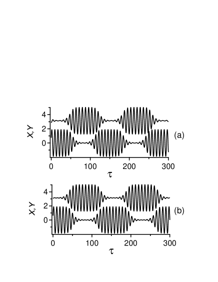
Figure 9: Motion of the particles as a function of the time $\tau=\omega_{0}t$, for $\alpha=0.5$ and $E=-1.02$, for initial conditions close to the unstable periodic orbits. In both plots, $X$ and $Y$ trajectories are centered on $0$, but for sake of clarity, the $Y$ trajectories have been shifted by $\pi$, so that they appear to be centered on $\pi$. The corresponding trajectories are on tori centered on (a) the antiphase periodic orbit and (b) a quadrature periodic orbit.

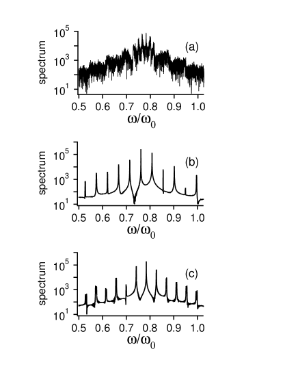
Figure 10: Spectrum of particle trajectories close to the unstable periodic cycles, in (a) the chaotic area, (b) on the side of the antiphase solution and (c) on the side of a quadrature solution.

We examine now the behavior of the system in the vicinity of the unstable solutions. As discussed in philo , the dynamics in the immediate vicinity of the separatrix is chaotic when the energy is large enough. Fig. 10a shows a typical spectrum with the characteristics of chaos, in particular a large continuous component. The existence of chaotic trajectories in the vicinity of the trivial solutions confirms the unstable nature of these solutions. However, the chaotic area remains marginal in the lattice we discuss here. For example, in Fig. 5, the chaotic area is so small that it cannot be visible at the scale of the representation.

Fig. 9 shows the temporal dynamics on tori passing close to the ($X=0$, $\dot{X}=0$) point, just outside the chaotic area, on the antiphase solution side in (a), and on the quadrature side in (b). As expected in the vicinity of an unstable solution, these dynamics do not seem to be linked to the solution itself. On the contrary, they appear as an evolution of the regimes generated by the corresponding stable periodic orbit. Indeed, they have the main characteristics of the regimes observed in the vicinity of the periodic cycles. In particular, the two regimes differ by the phase difference between the oscillations in $X$ and $Y$, and the amplitude modulations for the motion in $X$ and in $Y$ are always in antiphase, i.e. the particle oscillates for a while along the $X$-axis and then moves to the $Y$-axis, and vice-versa. Fig. 10b and 10c shows the spectra associated with these dynamics. The dynamics in the $X$ and $Y$ directions are still synchronized, with one main frequency and sidebands well below this main frequency. However, some differences appear as compared to the vicinity of the stable solutions: in particular, the amplitude of the sidebands is larger, with less than one order of magnitude as compared to the main frequency, and several harmonics have a non negligible amplitude.

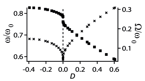
Figure 11: Evolution of the main frequency $\omega$ (squares) and the beating $\Omega$ (crosses) for different trajectories, for $\alpha=0.5$ and $E=-1.02$. Trajectories are identified through the point where they intersect a line linking the quadrature and the antiphase solution. $D$ is the distance between the intersection point and the separatrix. The quadrature (resp. antiphase) solution is in $D=-0.4$ (resp. $D=0.6$).

We have now a good picture of the motion of an atom in a well of our lattice. Whatever its energy is, its motion is mainly a periodic oscillation distorted by a slow drift. This drift vanishes on the periodic stable solutions, and increases when one moves away from these solutions. The frequency of the oscillation, together with that of the sidebands, evolve with the energy, but evolve also in the phase space of a given energy. Fig. 11 shows the evolution of the behavior when one moves away from the stable solutions, for $\alpha=0.5$ and $E=-1.02$. On the whole accessible phase space, the dynamics is still essentially an oscillation with the same frequency in both directions, perturbed by sidebands. Fig. 11 shows that the main frequency evolves continuously between the resonance frequencies of the different stable solutions. In particular, for the four domains delimited by the separatrix, the main frequency tends to that of the unstable solution for trajectories at the edge of the domain. The beating frequency also evolves monotonically in each domain, tending to zero when the separatrix is approached. So the transition between each periodic solution occurs without any discontinuity.

6 Conclusion

We have shown in philo that the nature and the complexity of the motion of an atom in an optical lattice – or similarly of a classical particle in the corresponding external potential – can change drastically as a function of the lattice properties. We study the fundamental mechanisms leading to so important differences in the dynamics, and especially the absence of chaos in the potential wells of a red detuned square optical lattice. We adopt an approach quite unusual in the domain of conservative chaos, because our aim is to find experimental tools able to characterize more precisely the complex conservative dynamics, and in particular able to distinguish between different complex behaviors. In square lattices, atoms traveling between sites follow two different chaotic behavior, depending on the lattice blue or red detuning. This difference probably originates in the behavior of atoms inside the wells: full chaos appears when the laser frequencies are blue detuned, whereas chaotic trajectories are quasi inexistent when they are red detuned. The former is not surprising: the edges of a well are far from harmonicity, and the coupling between the two directions, together with the nonlinearities, become very high. On the contrary, the mechanism leading to the absence of chaos in the latter needed to be clarified. We show here that synchronization between the motion in the two directions of space inhibits chaos, through a mechanism very similar to that of frequency locking in dissipative systems. Indeed, the frequencies in both directions of space are degenerate at the bottom of the well. For atoms with higher energies, the degeneracy should be broken, but the coupling overcomes the anharmonicity and leads to a motion with one single frequency. Synchronization is not strictly frequency locking, as our system is conservative, and there is no dissipation to compensate for frequency pulling. So the periodic oscillations are modulated in phase and in amplitude, i.e. the main frequency comes along with small sidebands. In the phase space, the amplitude modulation can increase, and even reach 100% in the vicinity of the unstable periodic orbits, but the description in terms of frequency locking remains valid on most of the phase space. Finally, in our conservative lattice, synchronization appears to be at the origin of the absence of chaos, following the same mechanisms as in dissipative systems. This intrinsic origin of this inhibition is not a local behavior, i.e. the lack of chaos will remain whatever the lattice parameters are, except for the lattice frequency. In particular, the quantum dynamics should be studied in another lattice, as e.g. the blue detuned square lattice, where chaos is fully developed.

This analysis shows that the dynamics of conservative systems can be characterized using deterministic tools rather than the traditional statistical approaches. Atoms in optical lattices are a good model system to apply these tools and test them on experiments. Future studies could refine the present results, in particular by checking that this approach is still valid when, at the main resonance, the frequencies in both spatial directions are not equal, but only multiple. This can be achieved with the blue detuned square lattice, by choosing adequately $\alpha.$

References

- (1) M. Greiner, O. Mandel, T. Esslinger, T. W. Hänsch and I. Bloch, Nature 415, 39 (2002)
- (2) B. Paredes, A. Widera, V. Murg, O. Mandel, S. Fölling, I. Cirac, G. V. Shlyapnikov, T. W. Hänsch and I. Bloch, Nature 429, 277 (2004)
- (3) W. H. Kuan, T. F. Jiang, and Szu-Cheng Cheng, Chin. J. Phys. 45 219 (2007)
- (4) D. Jaksch and P. Zoller, Ann. Phys. 315, 52 (2005)
- (5) O. Mandel, M. Greiner, A. Widera, T. Rom, T. W. Hänsch and I. Bloch, Nature 425, 937 (2003); K. G. H. Vollbrecht, E. Solano and J. I. Cirac, Phys. Rev. Lett. 93, 220502 (2004)
- (6) P. Douglas, S. Bergamini. and F. Renzoni, Phys. Rev. Lett. 96, 110601 (2006)
- (7) J. Jersblad, H. Ellmann, K. Støchkel, A. Kastberg, L. Sanchez-Palencia, and R. Kaiser, Phys. Rev. A 69 013410 (2004)
- (8) J. Billy, V. Josse, Z. C. Zuo, A. Bernard, B. Hambrecht, P. Lugan, D. Clement, L. Sanchez-Palencia, P. Bouyer and A. Aspect, Nature 453 891-894 (2008)
- (9) G. Roati, C. D’Errico, L. Fallani, M. Fattori, C. Fort, M. Zaccanti, G. Modugno, M. Modugno and M. Inguscio, Nature 453, 895 (2008)
- (10) J. Chabe, G. Lemarie, B. Gremaud, D. Delande, P. Szriftgiser, and J. C. Garreau, Phys. Rev. Lett. 101 255702 (2008)
- (11) D. A. Steck, V. Milner, W. H. Oskay, and M. G. Raizen, Phys. Rev. E 62, 3461 (2000)
- (12) H. Lignier, J. Chabe, D. Delande, J. C. Garreau and P. Szriftgiser, Phys. Rev. Lett 95, 234101 (2005)
- (13) A. L. Lichtenberg et M. A. Lieberman, “Regular and chaotic dynamics”, Springer Verlag, Berlin (1991)
- (14) H. Guo, Y. Wen and S. Feng, Phys. Rev. A 79, 035401 (2009)
- (15) D. K. Chaikovsky and G. M. Zaslavsky, Chaos 1, 463 (1991)
- (16) N. C. Panoiu, Chaos 10, 166 (2000)
- (17) D. Hennequin and Ph. Verkerk, arXiv:0906.2121 [physics.atom-ph]
- (18) E. Courtade, O. Houde, J.-F. Clément, P. Verkerk and D. Hennequin, Phys. Rev. A, 74 031403(R) (2006)
- (19) L. Guidoni and Ph. Verkerk, J. Opt. B: Quantum Semiclass. Opt. 1, R23 (1999)
- (20) L. Guidoni, C. Triche, P. Verkerk and G. Grynberg, Phys. Rev. Lett. 79, 3363 (1997)
- (21) M. Greiner, I. Bloch, O. Mandel, T. W. Hänsch, and T. Esslinger, Phys. Rev. Lett. 87 160405 (2001)