Neutral pion electroproduction in the resonance
region at high $Q^{2}$

Abstract

The process $ep\rightarrow ep\pi^{0}$ has been measured at $Q^{2}$ = 6.4 and 7.7 (GeV/c²)² in Jefferson Lab’s Hall C. Unpolarized differential cross sections are reported in the virtual photon-proton center of mass frame considering the process $\gamma^{\ast}p\rightarrow p\pi^{0}$. Various details relating to the background subtractions, radiative corrections and systematic errors are discussed. The usefulness of the data with regard to the measurement of the electromagnetic properties of the well known $\Delta(1232)$ resonance is covered in detail. Specifically considered are the electromagnetic and scalar-magnetic ratios $R_{EM}$ and $R_{SM}$ along with the magnetic transition form factor $G_{M}^{\ast}$. It is found that the rapid fall off of the $\Delta(1232)$ contribution continues into this region of momentum transfer and that other resonances may be making important contributions in this region.

I Physical Motivation

Electromagnetic elastic and transition form factors have historically proved essential in furthering the understanding of baryon structure and the concomitant degrees of freedom necessary to describe it. The spectra of baryon transition resonances led directly to the quark model, and the basic measurable static and dynamic properties of many excited baryon states were successfully described by the constituent quark model (CQM). Properties of charge and current distributions such as the charge radius were obtained from elastic electron scattering as a function of the 4-momentum transfer $q^{2}$.

By far the most studied of the resonances has been the $\Delta(1232)$, which has both spin and isospin quantum numbers of 3/2. It is the lowest lying excitation and it decays almost exclusively into the simple $N-\pi$  final state with a $p$-wave. It is relatively isolated from other resonances and is very strongly excited, almost completely saturating the unitary circle in an Argand plot. Since its spin is 3/2 it can be electromagnetically excited via three electromagnetic multipoles - $M1$, $E2$ and $S1$, which denote magnetic dipole, electric quadrupole and scalar dipole, respectively.

For real photons ($Q^{2}$=0) the $\Delta(1232)$ resonance (hereafter simply referred to as “the $\Delta$”) is nearly a pure $M1$ excitation. Early on this was explained in the framework of the SU(6) CQM as a magnetic spin-flip excitation of one of the nucleon’s quarks, which move in a spherically symmetric oscillator type potential Becchi and Morpurgo (1965). However, it is found that the $\Delta$ excitation also has small, but non-zero, components of $E2$ and $S1$ amplitudes. Near $Q^{2}$=0 it is found that the ratio $R_{EM}\equiv E2/M1\sim$ -0.02 to -0.03 . This non-zero $R_{EM}$ implies that the $N\to\Delta$ transition has an electric quadrupole moment and therefore the $\Delta$ is slightly deformed from sphericity. The splitting of the $\Delta$ mass from the nucleon has been interpreted Isgur and Karl (1978); Isgur et al. (1982) as arising from a color hyperfine interaction, which also induces the small electric quadrupole moment. The existence of this small distortion of shape has been alternatively described Sato and Lee (1996, 2001) as a non-spherical pion cloud, which is part of the sea quarks, surrounding the spherical quark core.

As $Q^{2}$ increases one begins to penetrate this cloud and access the core. The small wavelength virtual photons begin to resolve current quarks. The description of the process must evolve with with $Q^{2}$ as well. At the asymptotic limit, $Q^{2}\to\infty$, it is widely accepted that the pQCD approach should explain all exclusive reactions in which the entire process involves only the minimum Fock state configuration of quarks, which exchange the minimum number of gluons. For baryon elastic and transition form factors this implies three valence quarks exchanging two gluons, with helicity conservation at each vertex. The result is the so-called pQCD constituent scaling, which for baryons means the leading form factors should scale as $1/Q^{4}$. In addition to constituent scaling, the pQCD process requires helicity conservation for the overall process.

The question of how to describe exclusive reactions at $Q^{2}$ between zero and infinity is one of the major fields of study in nuclear physics today, and will be continue to be so in the foreseeable future. The present range of $Q^{2}$ over which baryon form factors can be studied in detail (aside from the elastic proton magnetic form factor $G_{Mp}$) is approximately from $0$ to around 8 (GeV/c²)², over which the wavelength of the probe varies from about 1 fm to less than 0.05 fm. Over such a large range of probe resolution it is not clear which models of description are most appropriate, and their ranges of relevance must also evolve.

The present analysis is concerned with the upper range of the available momentum transfers. There are several approaches which have been applied to the study of the exclusive reactions and baryon form factors in this kinematic range: pQCD; generalized parton distributions (GPD); light cone-sum rules (LCSR); lattice QCD (LQCD); and relativistic versions of the CQM. A review of the physics of resonances at high $Q^{2}$ can be found in Ref. Burkert et al. (2009), which also includes pertinent references. The important signatures relating to the onset of pQCD are the constituent scaling rules and helicity conservation. The scaling rules predict that the leading order $N\to\Delta$ transition form factor $G_{M}^{\ast}$, which is directly related to the dominant $M_{1+}$ multipole, scales as $1/Q^{4}$. Helicity conservation implies $R_{EM}=+1$. A further consequence of pQCD is that $R_{SM}$ be a constant. It would be very significant if $G_{M}^{\ast}$, $R_{EM}$, and $R_{SM}$ begin to approach these behaviors in the range $2.5\leq Q^{2}\leq 10.0$ (GeV/c²)². At intermediate values of $Q^{2}$ estimates have been made in terms of GPDs Stoler (1993), LCSRs Stoler (1993) large $N_{C}$ and chiral limits Pascalutsa and Vanderhaeghen (2006); Pascalutsa et al. (2007), and LQCD Alexandrou et al. (2005).

Earlier analysis of inclusive electron scattering data at SLAC Stoler (1993); Stuart et al. (1998) indicated that the $p\to\Delta$ form factor is decreasing with $Q^{2}$ at a slope steeper than pQCD scaling. Exclusive experiments Frolov et al. (1999); Joo et al. (2002); Ungaro et al. (2006) unambiguously show that one has not reached a kinematic region where pQCD contributions become dominant up to a momentum transfer of almost $Q^{2}=6$ (GeV/c²)². However, it is also possible that the data is beginning to show an interpolating behavior between the values at the currently accessible kinematic regions and the pQCD predictions. Some simple expectations have been put fourth based on the knowledge of the behaviors of other known form factors and specific pQCD predictions Carlson and Mukhopadhyay (1998).

The goal of this experiment was to measure the $N\to\Delta$ transition form factors at the highest possible momentum transfers and to confront current theoretical issues:

• Whether $G_{M}^{*}$ continues to fall anomalously fast as a function of $Q^{2}$, or whether it begins to approach the scaling behavior equivalent to the dipole form.

• Whether E2/M1 remains very small and negative, or whether it begins to turn positive, and asymptotically begin to approach +1.

• Whether S1/M1 also approaches a scaling behavior, constant with $Q^{2}$.

The data presented here will facilitate the examination of the $N\to\Delta$ amplitudes vis-a-vis the prediction of theoretical formalisms in this higher $Q^{2}$ but sub-pQCD kinematic region.

The new measurements reported here are for the reaction $\gamma^{\ast}+p\to\Delta^{+}\to p^{\prime}+\pi^{0}$. Previous experiments at Jefferson Lab for this reaction  Joo et al. (2002); Frolov et al. (1999); Ungaro et al. (2006) have provided data up $Q^{2}$ = 6.0 (GeV/c²)². The present experiment provides data of higher statistical accuracy at $Q^{2}$ = 6.4 and 7.7 (GeV/c²)², which was the highest possible at the beam energy of 5.5 GeV. In the future, the Jefferson Lab upgrade, will enable the experiments to approach $Q^{2}$ values near 13 or 14 (GeV/c²)².

II Electroproduction of $\pi^{0}$ Mesons

The single dynamical assumption which is made that makes kinematics simpler and indeed even allows straightforward parameterization of the dynamics is the single photon perturbative approximation. The results of this work relating to dynamical form factors are valid only to the extent that this approximation is satisfied. It is also very important to understand the process at hand in both the laboratory and the center of mass frames, to be defined in what follows. This is essential because the measuring apparatus are understood more fully in the lab frame while the dynamical predictions are simplified in the center of mass frame.

II.1 Definition of Coordinates and Cross Sections

We examine the differential cross section for a neutral pion from the following exclusive reaction:

$$e+p\rightarrow e^{\prime}+p^{\prime}+\pi^{0}.$$ (1)

The kinematics for such a process are displayed in Fig.1.

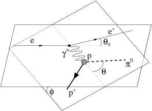
Figure 1: Lab frame neutral pion production. The symbol $e$ represents the incoming electron and $e^{\prime}$ the outgoing electron. The incoming and outgoing protons are denoted by $p$ and $p^{\prime}$, respectively. The symbol $\pi^{0}$ is the outgoing neutral pion and $\gamma^{\ast}$ is the exchanged photon.

In electroproduction of a single meson five kinematic variables are needed to specify the unpolarized reaction fully. Assuming that the energy of the incident electron, $E$, is known and that the target energy is simply $m_{p}$, these variables can be chosen to be the scattered electron energy $E^{\prime}$, the electron angles $\Omega_{e}$ and the meson angles $\Omega_{\pi}$. These completely specify the reaction. Given this convention, the 5-fold differential cross section can be obtained as a function of the mentioned variables. We express as many of the variables as possible through the use of Lorentz invariants. This procedure also makes one able to predict some simple dynamical effects from the covariant procedures for calculating QED matrix elements (the Feynman rules). Another advantage is that the lepton current portion will completely factorize in a frame-invariant way, which enables one to write the amplitudes in terms of only hadronic variables multiplied with some known (and frame invariant) QED factors. The most obvious new coordinate which is suggested from the lab frame kinematics and the canonical treatment of the elastic process is the momentum transfer from the electron to the target proton. In view of the one-photon exchange approximation this can be viewed as the 4-momentum of the exchanged virtual (off-shell) photon. This understanding of the 4-momentum transfer will be especially useful when moving to the center of mass frame.

$$q^{\mu}=k^{\mu}-k^{\prime\mu}$$ (2)

The symbol $k$ is the 4-momentum of the incoming electron and $k^{\prime}$ is the 4-momentum of the outgoing electron. Defining the incoming proton 4-momentum to be $p$ and the outgoing to be $p^{\prime}$, the two electron invariants become the following.

$$Q^{2} \equiv-q^{2}=2EE^{\prime}(1-\cos{\theta_{e}})$$ (3)

$$W \equiv\sqrt{(q+p)^{2}}=\sqrt{m_{p}^{2}+2q^{0}m_{p}-Q^{2}}$$

The rightmost equalities in Eq. 3 hold in the lab frame. Another experimentally useful invariant is the missing mass, $M_{x}^{2}$, which is the square of the undetected 4-momentum. In the present case this is:

$$M_{x}^{2}=(q+p-p^{\prime})^{2}.$$ (4)

The dependence on the leptonic variables is now completely in terms of invariants which can be calculated in any frame.

It is desirable to move to the hadron-virtual photon center of mass frame. Kinematically this is desirable because it essentially replaces three body final state with the two body version. Dynamical considerations for the pure QED portion of the matrix element must, however, be taken into account. As previously indicated, the lepton current portion of the matrix element will factorize. Lorentz boosting to the center of mass along the direction of the momentum transfer enables one to treat the hadronic cross section as the interaction of a virtual photon with a target hadron and treat the leptonic current as a prefactor to the amplitude which is a function of the Lorentz invariants $Q^{2}$ and $W$. The center of mass frame is shown in Fig. 2.

Figure 2: Center of mass frame neutral pion production.

An asterisk denotes a center of mass quantity except when symbolically referring to a photon in which case an asterisk (as in $\gamma^{\ast}$) denotes that the photon is virtual (off-shell).

The details of the lepton current factorization are reviewed in Refs. Lyth (1978); Dombey (1969); Pilkuhn (1967). The result is that the 5-fold differential cross section can be written as follows.

$$\frac{d\sigma}{dE^{\prime}d\Omega_{e}d\Omega^{\,\ast}_{\pi}}=\Gamma\frac{d\sigma^{\gamma^{\ast}}}{d\Omega^{\,\ast}_{\pi}}$$ (5)

The factor $\Gamma$ in Eq. 5 is the virtual photon flux factor. In the Hand convention Hand (1963) this reads:

$$\Gamma \equiv\frac{\alpha}{2\pi^{2}}\frac{E^{\prime}}{E}\frac{(W^{2}-m_{p}^{2})}{2m_{p}Q^{2}}\frac{1}{1-\epsilon}$$ (6)

$$\epsilon \equiv\left(1+2\frac{|\mathbf{q}|^{2}}{Q^{2}}\tan^{2}{\frac{\theta_{e}}{2}}\right)^{-1},$$

in which $\epsilon$ describes the ratio of longitudinal to transverse polarization of the virtual photons. Because of the structure of the virtual photon density matrix Dombey (1969); Villano (2007), one can write explicitly the $\phi^{\,\ast}$ dependence of the center of mass cross section in terms of the transverse (T), longitudinal (L), transverse-transverse interference (TT) and longitudinal-transverse interference (LT) portions of the interaction.

$$\frac{d\sigma^{\gamma^{\ast}}}{d\Omega^{\,\ast}_{\pi}}=\sigma_{T}+\epsilon\sigma_{L}+\epsilon\sigma_{TT}\cos{2\phi^{\,\ast}}+\sqrt{2\epsilon(1+\epsilon)}\sigma_{LT}\cos{\phi^{\,\ast}}$$ (7)

The goal of the experiment is to obtain the center of mass pion differential cross sections and interpret all of the components displayed in Eq. 7 in terms of multipole amplitudes from the pion production data in this work.

III Experimental Overview

The experiment was carried out in the Jefferson Laboratory Hall C using a two-spectrometer setup for detection of outgoing electrons and protons.

A schematic of the Jefferson Lab Hall C setup is shown in Fig. 3. The hall is equipped with two magnetic spectrometers: the High Momentum Spectrometer (HMS) and the Short Orbit Spectrometer (SOS). The target consisted of liquid hydrogen (LH₂), at a temperature of 19.0 K.

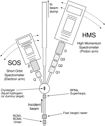
Figure 3: Plan view of the experimental layout in Hall C (from Ref. Blok et al. (2008)). The symbols Q, Q1, Q2 and Q3 denote quadrupole magnets, D denotes forward bending dipole and $\rm\bar{D}$ denotes reverse bending dipole.

Exclusive electroproduction data for the process $ep\rightarrow epX$ was gathered in the spring of 2003 run period. The electron beam energy was about 5.5 GeV and the $Q^{2}$ values were 6.4 and 7.7 (GeV/c²)² at the $\Delta$ resonance.

The HMS was used to measure the proton momentum and angles while the SOS was used to measure the electron momentum and angles. Details of the spectrometer properties and detector packages as used in this experiment can be found in Ref. Villano (2007). Though the magnetic spectrometers have a small acceptance compared to the acceptance of a $4\pi$ detector, the relatively low values of $W$ and high values of $Q^{2}$ cause protons to emerge in a rather narrow cone around the $\mathbf{q}$ vector. Full coverage can thus be obtained in the center of mass variables by using several HMS angle and momentum scans. The spectrometer settings for the experiment are listed in Tbl. 1.

Electron Arm		Proton Arm
$p_{\mathrm{SOS}}$	$\theta_{\mathrm{SOS}}$	$p_{\mathrm{HMS}}$	$\theta_{\mathrm{HMS}}$
GeV/c	degrees	GeV/c	degrees
		4.70†	18.0, 15.0
		4.50†	19.5, 16.5, 13.5, 11.2
		3.90†	21.0, 18.0, 15.0, 12.0
		3.73†	22.5, 19.5, 16.5, 13.5, 11.2
1.74	47.5	3.24†	24.0, 21.0, 18.0, 15.0, 12.0
		3.10†	22.5, 19.5, 16.5, 13.5, 11.2
		2.69†	24.0, 21.0, 18.0, 15.0, 12.0
		2.57†	22.5, 19.5, 16.5, 13.5, 11.2
		2.23†	21.0, 18.0, 15.0, 12.0
		2.13†	22.5, 19.5, 16.5, 13.5
		4.70	11.2
		4.50	14.2
1.04	70.0	3.90	11.2
		3.73	14.2, 11.2
		3.24	11.2

Table 1: The kinematic settings of the two spectrometers. The beam energy is nominally 5.5 GeV.

III.1 Beamline and Target

The experiment depends on knowing to a reasonable accuracy the beam energy, and current. Prior to the interaction in the target the electron beam traverses the beam current monitoring, beam energy measurement and beam raster devices.

In standard running, the beam is tuned in an achromatic mode through an arc which consists of eight dipoles and is located just before the beam enters Hall C. To measure the beam energy, the beam is tuned to a dispersive mode through the arc dipoles. The current in the arc dipole magnets is varied until the beam is centered at the exit of the dipole arc. The relationship between the current in the arc dipoles and the field integral is known from previous measurements. The angle and position of the beam when entering and exiting the arc are measured and used to determine the correct path length through the arc dipoles. The relative uncertainty on the beam energy measurement is 5$\times$10^-4 which is due to uncertainty in the field integral and in the path length through the arc dipoles. Ref. Yan et al. (1993) is a detailed description of the beam energy measurement technique. The beam energy measurement was done only once during the experiment, since the measurement interrupts regular data taking. To monitor changes in the beam energy during the experiment relative to the arc energy measurement, the positions and angles of the beam in the arc dipoles are measured throughout experiment and the beam energy is determined continuously. The beam energy varied during the first quarter of the experiment. The beam energy varied from 5.501 GeV to as low as 5.492 GeV. After this period, the beam energy was stable at 5.499 GeV. The small beam energy difference was taken into account in all simulation work and data reconstruction. Since results are not reported as a function of beam energy and the values of kinematics were calculated with the appropriate value for $E$, the beam energy is stated to be 5.5 GeV throughout this work when listing kinematics.

The beam current measurement is accomplished by using two beam current monitors (BCMs) positioned along the beam line. These current monitors are quite stable but do not have the ability to make an accurate absolute measurement. An additional current monitor, the Unser monitor, has a very stable gain but an offset that drifts considerably on short time scales Unser (1981), experiencing typical drifts of 3 $\mu$A. The solution used in this experiment was to extract the Unser monitor zero at various intervals during the experiment by ramping the beam current down in several steps. The BCMs, which are more stable but lack the absolute accuracy of the Unser, are then calibrated with the Unser monitor. This method was measured to be stable to 0.2% from run-to-run and had an overall accuracy of 0.5% on the charge measurement Blok et al. (2008).

After several current monitors on the beam line there is the fast raster system Yan et al. (1995). The Jefferson lab electron beam has very small spacial extent and therefore would induce significant boiling in cryogenic targets if the beam were allowed to impinge on the target for too long at a current of a few to several tens of microamps. For this reason, Hall C uses the fast raster which sweeps the beam uniformly over a square pattern on the target. The size of this pattern is typically $\pm$1.2 mm in the horizontal and vertical directions.

It should also be noted that the beam itself has a periodic time structure due to the RF techniques used to create and accelerate the beam. For the Jefferson Lab accelerator the frequency of this structure (corresponding to the excitation frequency of the cryogenic accelerator cavities) is 1497 MHz which corresponds to beam pulses which are about 668 ps apart. The beam is delivered to each hall by a kicker magnet which moves a third of the beam into each of the three hall beam pipes. Therefore when the beam arrives in each hall it will have bunches which are separated by roughly 2 ns. This intrinsic beam structure was important for subtracting coincidence spectrometer events which have two particles that do not correlate to the same beam bunch.

We turn now to the target specifications. The geometry of the target is especially important because of the possibility of electron scattering interactions in the target walls. The LH₂ target was kept in a constant cooling loop with a temperature of 19.0 K and pressure of 24 psi. At this temperature and pressure, the density of liquid hydrogen is 0.0723 g/cm³. The target ladder for the experiment contained several other targets along with a “dummy” target which was used for measuring the contribution to the data due to scattering in the target walls. This experiment used the LH₂ target and the Al dummy only. The target cell was cylindrical and 4.013$\pm$0.008 cm in diameter, made of 7075 aluminum with the beam impinging on the non-circular face. The thickness of the target cell was measured at four places around the cylinder Meekins (2003) and the results average to 0.1330 $\pm$ 0.0013 mm. There was a beam offset of 3 mm from the center of the cell so that the active length of the target included 3.941 cm of liquid. Electron radiation from this material was included in the Monte Carlo simulation used for the data analysis.

III.2 Detector Properties

The spectrometer coordinate system is defined such that the “z” axis is along the central axis of the spectrometer, “x” axis points in the positive dispersive direction and the “y” is perpendicular to the dispersive plane defined by the choice of a right handed coordinate system. Figure 4 shows the coordinate systems of both the SOS and HMS spectrometers. Both the focal plane and target quantities use this coordinate system for detected particles. In particular the change in the x or y coordinates per unit change in the z coordinate is used to calculate angles.

Figure 4: Spectrometer coordinate systems. The octagonal shapes represent the boundaries of the collimators at the entrances of the first quadrupole magnets of each spectrometer.

The entrances to the spectrometers are equipped with collimators having different dimensions for the HMS and the SOS. The octagonal shape of the collimators are displayed in Fig. 4 centered around the coordinate axes. The flight distance from the target to the collimator is 166.4 cm for the HMS and 126.3 cm for the SOS spectrometer. Each of the collimators are 6.3 cm thick and with beveled interiors so that exit openings are slightly larger than the entrance openings.

The HMS and SOS use momentum dispersion due to dipole magnetic fields in order to analyze the momentum of particles. Different momenta will pass through at different positions inside the detector hut on a two dimensional surface referred to as the focal plane.

The magnet configuration for the HMS is $QQQD$ (three quadrupoles then a dipole) and the configuration for the SOS spectrometer is $QD\bar{D}$, where the bar denotes a central bend angle in the opposite direction. The quadrupoles are used as focusing elements in general to allow the apparatus to accept events which would hit the spectrometer material had they not been focused prior to bending Green (2000). Both the HMS and SOS spectrometers used a point-to-point magnetic configuration, wherein particles which originate from a common point with common momenta will be focused to the same point on the focal plane. The magnets in the spectrometer are typically modeled by transport matrices in phase space where the matrix elements are fitted to data or obtained from a precise field map. Procedures for the optimization of the matrix elements for the magnets in Hall C have been refined over the years Dutta and Welch (1996); Blok et al. (2008). The SOS dipole magnet saturates above about 1 GeV/c in momentum so that a separate transport matrix had to be used for the 1.74 GeV/c (low $Q^{2}$) setting in the current experiment. The HMS had the same magnet matrix for all settings. This fact leads to a somewhat poorer knowledge of the SOS acceptance than the HMS acceptance which can be checked by measuring inclusive data in each spectrometer. The SOS acceptance was studied by using inclusive electron scattering and results are presented in Ref. Dalton et al. (2009). The HMS acceptance has been extensively studied in electron inclusive scattering experiments Christy et al. (2004); Tvaskis et al. (2007).

Figure 5 shows the typical detector package which is utilized in each spectrometer hut. Drift chambers are located on either side of the focal plane in each spectrometer and are shown schematically in Fig. 5. The drift chambers are used to determine the detected particle’s position and direction in each spectrometer’s focal plane. The rest of the detector package is located after the last drift chamber.

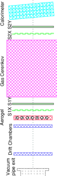
Figure 5: (color online) Typical spectrometer detector package. The graphic was taken from Ref. Blok et al. (2008). Particles travel from left to right.

The two sets of X-Y hodoscopes are shown on either side of the gas Čerenkov detector. These are labeled S1X, S1Y, S2X and S2Y in order along $+\hat{\mathbf{z}}$, with the X or Y label referring to the orientation of the scintillator strips. The hodoscopes were used for the electronics trigger in a 3-out-of-4 configuration, that is, a pretrigger is generated if 3 out of 4 of the hodoscope planes fire.

The basic electronics selection mechanisms and read out scheme is represented in Fig. 6. The scintillator bars on the four hodoscope X or Y planes were read out at each end and used to create a pretrigger. A signal on either edge of the bars give an electronic logical true if any of these bars fire. As Fig. 6 indicates, these pretriggers were then passed to a programmable module which decides which kind(s) of data acquisition triggers to produce. The so-called “8LM” programmable module will not produce a data acquisition (DAQ) trigger if it receives a “busy” signal from the DAQ, indicating that the DAQ is not ready for another event. When the DAQ was not busy, the 8LM module produced HMS, SOS, or coincidence triggers which were passed along to the trigger supervisor. The coincidence trigger was the logical “and” of the HMS and SOS triggers which require a 3 out of 4 scintillator plane event in each spectrometer. The timing between the SOS and HMS pretriggers was adjusted so that there was an overlap for a coincidence trigger.

Figure 6: Simplified representation of the electronics and data acquisition system for experiment E01-002.

The trigger supervisor controls the DAQ by dispensing gates to the ADC and TDC modules only when a valid event is present and the DAQ is not already busy digitizing a previous event. The trigger supervisor also performed any necessary prescaling of the signals. The prescaling allows the DAQ to skip some set number of events, or, read only every $n^{th}$ event where $n$ is the prescale factor. For example SOS singles prescale factors used in this work were 1, 2, 3 and 5. The HMS singles have prescale factors which ranged from 100 to a few thousand at the low hadron momentum settings where $\pi^{+}$ production is copious. After the appropriate gates are dispensed for the appropriate triggers, the ADC and TDC modules (located in FastBus crates) will begin to digitize all relevant information concerning analog photomultiplier signals and time difference signals.

After being triggered the computer DAQ system digitized and stored the information from all of the detectors and monitors. The Jefferson Lab CODA Abbott et al. (2004) event builder was used to retrieve all relevant information from the ADC and TDC modules while storing event information on disk and/or on tape. Internet connections were used to communicate with the CPUs which were storing the ADC or TDC results.

Several data restrictions were made simply to ensure that the analyzed events include only ones where the SOS spectrometer recorded an electron event, the HMS spectrometer recorded a proton event and that these events are in coincidence.

Before the particle identification selections were made, however, the so-called “fiducial volume” was restricted to ensure that we use parts of the spectrometer focal plane which are well understood and avoid optics ambiguities. This allows the acceptance to be well modeled by Monte Carlo techniques. The fiducial restrictions were:

$$-20.0\leq \;X_{s}\leq 22.0\quad(\text{mm})$$ (8)

$$y^{\prime}_{min}\leq \;y^{\prime}_{s}\leq y^{\prime}_{max}$$

$$-18.0\leq \;\delta_{s}\leq 18.0\quad(\%)$$

$$-9.0\leq \;\delta_{h}\leq 9.0\quad(\%).$$

The symbols $y^{\prime}_{min}$ and $y^{\prime}_{max}$ are defined as follows.

$$y^{\prime}_{min} \equiv\frac{1}{1000}(-125.0+4.25\delta_{s}+64.0y_{s}-1.7\delta_{s}y_{s})$$

$$y^{\prime}_{max} \equiv\frac{1}{1000}(125.0-4.25\delta_{s}+64.0y_{s}-1.7\delta_{s}y_{s})$$

The symbol $\delta_{s}$ is defined as $(p-p_{c})/p$ with $p_{c}$ the central momentum in the SOS spectrometer and $p$ the detected particle momentum, $\delta_{h}$ is the analogous quantity for the HMS, $y_{s}$ is the SOS “y” position at the target, $X_{s}$ is the SOS “x” position at the focal plane, and $y^{\prime}_{s}$ is the SOS “y” angle at the target. A further fiducial restriction is made by removing events which reconstruct to outside either of the collimator apertures.

The particle identification restrictions include two restrictions to identify electrons in the SOS spectrometer along with a timing restriction to verify that the HMS detects a coincident proton. Figure 7 displays the HMS momentum vs. the corrected time signal called “coincidence time,” $t^{\star}_{c}$. The corrected time signal is constructed so that the proton events arrive at zero relative time independent of momentum. The figure displays the relative timing curves for other possible HMS contaminants. One can see that the $\pi^{+}$ signal is largest but still easily separated from the proton signal.

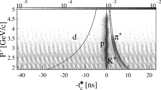
Figure 7: The “relative” $t^{\star}_{c}$ vs. hadron momentum for coincidence data normalized to make the proton’s time constant for all proton momenta.

The particle identification requirements are listed in Eq. 9 where the coincidence time is relative to the center of the proton peak.

$$|t^{\star}_{c}| \leq 1.5\quad(\text{ns})$$ (9)

$$\epsilon_{s} \geq 0.8$$

$$N^{\gamma}_{s} \geq 0.5$$

The variable $\epsilon_{s}$ represents the energy deposited in the SOS calorimeter divided by the particle momentum. The symbol $N^{\gamma}_{s}$ is the number of Čerenkov photons detected in the SOS.

III.3 Data Overview

It is useful to examine the overall results of the experiment to obtain intuition about backgrounds and cuts. The most natural distributions to look at are the missing mass, $M_{x}^{2}$, and invariant mass, $W$, distributions in Fig. 8. The invariant mass is that of the virtual photon-nucleon system and was quantified in Eq. 3. The missing mass distribution shows peaks corresponding to exclusive single mesons and continua due to multi-meson production and background. The invariant mass distribution indicates along which regions of invariant mass the meson events come from. Clear correlations between $W$ and $M_{x}^{2}$ can be seen in the figure. Further, one can see that $\pi^{0}$ production peaks at the $\Delta(1232)$ resonance and $\eta$ at the $S_{11}(1535)$ resonance. It should be noted that the $\Delta(1232)$ resonance is by no means the only source of $\pi^{0}$ production, whereas the $S_{11}(1535)$ dominates the $\eta$ production in the present region of $W$.

Figure 8: Upper panel: the missing mass distribution. The shaded regions highlight the peaks corresponding to $\pi^{0}$, $\eta$ and $\omega$ production. Lower panel: the $W$ distribution corresponding to the events in the upper panel. the shaded regions in the lower panel correspond to events in the shaded region of the upper panel. Each of the plots report the number of counts normalized to the total charge in millicoulombs (mC).

The invariant mass thresholds for $\pi^{0}$, $\eta$ and $\omega$ production are 1073.3, 1486.1 and 1720.9 MeV respectively. The two pion production threshold is at $M_{x}^{2}=$0.0729 (GeV/c²)², above the $\pi^{0}$ production analysis restrictions used in the present work.

IV Background Subtractions

Not all of the events present in the raw data acquisition represent the physical process of interest. One therefore must remove or modify a significant amount of events before the analysis can proceed. These modifications of the data set come in several varieties including background subtraction, and data corrections. Each of these modifications are considered in turn with specific attention given to radiative corrections on the pion production amplitudes, which have a physical origin distinct from any detector effects.

IV.1 Radiative Background Processes

There are two types of radiative processes which need to be treated. Radiative elastic scattering gives a background to the $\pi^{0}$ peak in the missing mass spectrum. Radiative processes accompanying $\pi^{0}$ electroproduction deplete the number of events under the single $\pi^{0}$ missing mass peak.

This section concerns elastic radiative processes which may “masquerade” as pion electroproduction processes in data analysis. The elastic radiative process is represented in Eq. 10.

$$e+p\rightarrow e^{\prime}+p^{\prime}+\gamma$$ (10)

The $\pi^{0}$ electroproduction process is:

$$e+p\rightarrow e^{\prime}+p^{\prime}+\pi^{0}$$ (11)

and is, in principle, easily distinguished from the radiative process but because of finite detector resolutions care must be taken in separating the two.

The missing mass for this work is always calculated by summing the 4-momenta of the incoming and outgoing measured particles. With the standard kinematic conventions one has that $p_{m}^{2}=(k+p-k^{\prime}-p^{\prime})^{2}=M_{x}^{2}$. For elastic scattering, or the case where a single photon is radiated, $M_{x}^{2}=0$. The low mass of the $\pi^{0}$, $m_{\pi}^{2}\sim$ 0.018 (GeV/c²)², makes it difficult to separate from processes which have $M_{x}^{2}=0$. This is because of experimental resolution effects on the calculated missing momenta. The result is that the pion and radiative missing mass peaks will have an apparent broadening and, depending on $Q^{2}$ and $W$, the peaks may overlap. Generally speaking, the widths of the $M_{x}^{2}$ peaks are smallest for $W$ near the elastic peak and become larger with increasing $W$, so that in the region at or above the peak of the $\Delta(1232)$ there is a significant overlap of the $\pi^{0}$ and elastic missing mass peaks.

The radiative processes of QED have been studied for many years and an authoritative body of literature exists on the subject Maximon and Tjon (2000); Walecka (2001); Ent et al. (2001); Mo and Tsai (1969). Some of the major developments were the treatment of the infrared divergences and the re-summing of the QED expansion for multiple low-energy photons Yennie and Suura (1957). In this work the resulting angular and energy dependences of the radiative events are used to remove elastic radiative contamination from the pion production peak.

The amplitudes for initial or final state radiation can be calculated exactly using well known QED techniques and suitable parameterizations of proton elastic form factors Rosenbluth (1950). An immediate result of the photon radiation amplitudes is that there are strong peaks along the direction of the outgoing or incoming charged particles. Since the proton is about two thousand times more massive than the electron, the radiation will be predominantly along the directions of the incoming and outgoing electrons. This fact is an important kinematic reality that allows this contribution to be excluded fairly efficiently even without simulation of the radiative events.

The result of this tight angular distribution is that elastic radiative events, though they might have a recorded invariant energy in the $\Delta$ region will emerge very nearly in the electron scattering plane. In other words they will peak around $\phi^{\,\ast}$= $\pi$. In contrast, the plane of emitted protons and pions can be distributed around the electron scattering plane with $\delta\phi^{\,\ast}\sim 2\pi$. By cuts close to $\phi^{\,\ast}$= $\pi$ one eliminates nearly all the elastic radiated events while losing only a small fraction of non-radiated events. The binning used for the data is such that removing events in a tight angular region around $\phi^{\,\ast}$= $\pi$ will not have an adverse affect on the data quality. The two dimensional distribution displayed in Fig. 9 shows the elastic radiative events around zero missing mass spreading to lower and higher missing mass in a narrow line along $\phi^{\,\ast}$= $\pi$.

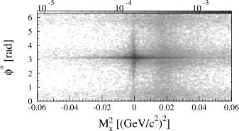
Figure 9: $M_{x}^{2}$ vs. $\phi^{\,\ast}$ with only standard cuts and $W>$ 1.1 GeV applied. Events in the vertical band near $M_{x}^{2}=$ 0.018 (GeV/c²)² are from single $\pi^{0}$ electroproduction. Elastic events form a peak around $M_{x}^{2}=$ 0 and elastic radiative events form a broad band centered on $\phi^{\,\ast}=\pi$.

A composition of two exponential contours were chosen to eliminate the unwanted radiative events while impacting the signal events minimally. For this purpose an envelope equation $\tilde{\phi}(M_{x}^{2})$ is defined with several adjustable parameters.

$$|\tilde{\phi}(M_{x}^{2})|=\begin{cases}\left(\frac{\phi_{g}}{e^{-\gamma^{\prime}m_{g}}}\right)e^{-\gamma^{\prime}M_{x}^{2}}+\pi,&M_{x}^{2}<m_{t}\\ \left(\frac{\phi_{t}}{e^{-\gamma m_{t}}}\right)e^{-\gamma M_{x}^{2}}+\pi,&M_{x}^{2}\geq m_{t}\end{cases}$$ (12)

With the definition:

$$\gamma^{\prime}\equiv\left(\frac{1}{m_{t}}\ln{\frac{\phi_{g}}{\phi_{t}}}\right).$$ (13)

The missing mass resolution becomes poorer with increasing $W$ since the range of protons are emitted with a greater variation in momenta over a greater range of $\cos{\theta^{\,\ast}}$, and detected over a larger range of the spectrometer focal plane. Thus, the parameters which define the elastic radiative rejection should be functions of the azimuthal angle.

$\cos{\theta^{\,\ast}}$ range	$\phi_{t}$	$\phi_{g}$	$\gamma$	$m_{t}$ (GeV2)	$m_{g}$ (GeV2)
-1.0 $\leq\cos{\theta^{\,\ast}}<$ -0.4	0.4	3.0	30.0	0.006	0.0
-0.4 $\leq\cos{\theta^{\,\ast}}<$ 0.25	0.19	.20	20.0	0.006	0.0
0.25 $\leq\cos{\theta^{\,\ast}}<$ 1.0	0.19	.20	20.0	0.006	0.0

Table 2: Radiative rejection in different $\cos{\theta^{\,\ast}}$ bins.

Table 2 displays the elastic radiative rejection parameters in each region of the azimuthal angle. The binning in the table was chosen empirically in order to reflect the variation in $\phi^{\,\ast}$ vs. $M_{x}^{2}$ of the radiative tail distribution.

The two dimensional radiative rejection depends on the missing mass ($M_{x}^{2}$). In addition to this two dimensional restriction there is a simpler missing mass restriction that should be applied for the final analysis to be sure that only pion production events are selected. The missing mass requirement is a standard one dimensional restriction, made with a width that is a function of $\cos{\theta^{\,\ast}}$ to account for the resolution change in the double arm measurement. The value of $\cos{\theta^{\,\ast}}$ is taken to be at the center of the kinematic bin. The specific form is determined by an empirical fit to the missing mass widths.

$$M^{2}_{min} =(-0.0118\cos{\theta^{\,\ast}}+0.00014)$$

$$M^{2}_{max} =(0.0136\cos{\theta^{\,\ast}}+0.04134)$$

The missing mass requirement can then be expressed as the following:

$$M^{2}_{min}\leq M^{2}_{x}\leq M^{2}_{max}.$$ (14)

Figure 10 displays this missing mass requirement for several kinematic bins.

Figure 10: Experimental missing mass ($M_{X}^{2}$) distributions for ten $\cos{\theta^{\,\ast}}$ bins after the cuts in Tbl. 2 were applied. The histograms are arbitrarily normalized and include all $\phi^{\,\ast}$ values. The dashed vertical lines represent the regions around the $\pi^{0}$ peaks outside of which the events are rejected by the further $\cos{\theta^{\,\ast}}$ cuts of Eq. 14. The vertical scale of the plots displays the number of events normalized to the maximum bin content of each histogram.

In summary, the radiative elastic events have been removed from the current data set via a restriction on the kinematic variables. Since the missing mass spectra look quite clean after the subtraction, no further subtractions were needed for this background.

IV.2 Background Simulation for $p(e,e^{\prime}p)\gamma$

We simulated the $p(e,e^{\prime}p)\gamma$ process with a Monte Carlo method similar to that for the exclusive pion production. The angle peaking approximation was used to generate photons along the direction of incident or scattered electron (or both) with a probability distribution based on the formulas of Ref. Mo and Tsai (1969). The elementary cross section was modeled using the form factor parameterization of Ref. Bosted (1995). The number of events below pion threshold $W<1.08$ GeV was found to be in good agreement with those observed in this experiment. The distribution of events for $W>1.1$ GeV is plotted in three bins of $\cos{\theta^{\,\ast}}$ in the upper panels of Fig. 11 as a function of $M_{x}^{2}$ and $\phi^{\,\ast}$. The distributions are strongly peaked near $\phi^{\,\ast}=\pi$, as expected, and for forward angle protons, a strong peak is also evident near $M_{x}^{2}=0$. The curves on the plots show the cuts used to reduce the background from events near $\phi^{\,\ast}=\pi$ to a negligible level (less than 1% contamination of the $\pi^{0}$ sample, in the worst case). The functional form of the $M_{x}^{2}$-dependent cuts on $\phi^{\,\ast}$ was described in the previous section and the parameters were listed in Tbl. 2. The vertical dashed lines show the cuts used to remove the events near $M_{x}^{2}=0$ (and also to reduce the background from accidental coincidences).

Figure 11: Comparison of the radiative rejections with simulated elastic radiative events. The upper panels a), b) and c) are the simulated elastic radiative events with the cuts from Sec. IV.1 superimposed. The lower panels d), e) and f) repeat the data distributions for comparison. Panels a) and d) display the rejection for the 0.25 $\leq\cos{\theta^{\,\ast}}\leq$ 1.0 range. The panels b) and e) show the rejection curve for the -0.4 $\leq\cos{\theta^{\,\ast}}\leq$ 0.25 range. The panels c) and f) show the rejection curve for the -1.0 $\leq\cos{\theta^{\,\ast}}\leq$ -0.4 range. The dotted lines represent the additional $M_{x}^{2}$ restriction placed on the data in the analysis.

The actual distributions of events from this experiment versus $M_{x}^{2}$ and $\phi^{\,\ast}$ are repeated for comparison in the lower panels of Fig. 11. It can be seen that distributions very similar to those in the upper panels (from the simulation) are super-imposed on a flatter distribution from $\pi^{0}$ production, and a very flat distribution from accidental coincidences. It was checked that the magnitude of the simulated $p(e,e^{\prime}p)\gamma$ background was within 20% to 30% of the observed distributions. Since the background is so concentrated in a narrow region of $\phi^{\,\ast}$, it was decided to not subtract this background, but simply reduce it to a negligible level with the cuts described above. As a further check that the simulation matched the $M_{x}$ and $\phi^{\,\ast}$ resolutions of the experiments, the cuts were varied over a reasonable range, and no significant change in the cross section was observed. This is described further in Section VI

IV.3 Data Corrections

There are several corrections that must be made to the data that are unrelated to competing physical processes but are a result of the apparatus used for the measurement. For the current measurement these include “accidental” coincidence counts, missed counts due to inefficiency in the data collection process, particle tracking inefficiencies and proton absorption. Still other effects are observed to be small and so they are not explicitly corrected for but are included in the systematic error estimation. These include target boiling, target window scattering, and calibration inefficiencies.

Because a radio frequency (RF) pulsed beam has a characteristic timing structure, there is a possibility that a coincidence trigger can originate from two particles from different beam bunches. The electron beam at Jefferson Lab’s continuous electron beam accelerator has a regular periodic structure in time and this structure helps identify contamination from non-vertex electrons or hadrons. The “coincidence time” is a variable which measures when the HMS detector triggers (proton detection) with respect to when the SOS detector triggered. Fig. 12 shows the distribution of events in this timing variable.

Figure 12: Timing spectrum of coincidence events. The cross-hatched insert shows the typical analysis cut made on this spectrum. The diagonal shading shows typical RF beam structure populated with accidental coincidences. Proton coincidence events are normalized to appear at zero with lighter particle coincidences appearing to the right.

In Fig. 12, the large peak corresponds to proton coincident events and the large shoulder at higher coincidence time are $\pi^{+}$ events (there are enough $\pi^{+}$ events to analyze the charged pion production cross section). Outside of these peaks the periodic structures correspond to events which make a coincidence between two different RF bunches. These events are the “accidental” coincidences and are removed by using data from far out on the coincidence time spectrum and assuming that the structure persists through the proton peak. The events used for the subtraction were taken from the diagonally shaded region in Fig. 12 and were far from the region where one could expect deuteron coincidences.

A more sophisticated extraction of the underlying beam structure might have been warranted if there were higher rates for these other positively charged hadrons. The accidental count subtraction was typically small, $<1.0$%, with the worst case being 8.0% which occurred in only one kinematic bin.

Although the timing selections select events in the SOS and HMS spectrometers that are coincident, the electronics and computers which allow this data to be recorded have associated deadtimes. The resulting computer and electronic deadtimes have been quantified.

The electronic deadtime was measured on a run by run basis using a scalar read out of different gate generators which are triggered by the coincidence event pulse. Having a rate measurement for several different generated gate widths allows extrapolation to the zero gate width and thus a determination of the electronic deadtime Gaskell (2003); Villano (2007). In the present experiment the electronic deadtime was 0.49% on average.

The computer dead time was calculated from the ratio of pretriggers $N_{pre}$ to the number of triggers $N_{trig}$ created programmable module. Recalling Fig. 6, one can see that this comparison gives a direct measure of the average percentage of counts which encountered a busy programmable logic module. The computer dead time $\frac{N_{pre}}{N_{trig}}$ was 6.8% on average for this experiment and data was corrected on a run-by-run basis.

The efficiency of tracking in the SOS and HMS drift chambers was defined as the probability of finding a valid track for a particle identified as a electron (proton) for the SOS (HMS). For the SOS, the rates in the focal plane were 10 kHz or lower and the tracking efficiency averaged about 99.5%. With the HMS at more forward angles, the rates in the HMS focal plane were higher and ranged from 40 kHz to 400 kHz at the most forward angle. A study Horn et al. (2007) of the tracking efficiency of the HMS drift chambers found a linear fall-off in the tracking efficiency with increasing rates at focal plane which was related to increased likelihood of multiple tracks. The HMS tracking efficiency was 95.2% when averaged over all kinematic settings.

Because the proton interacts strongly there is a reasonable probability that it will interact with the nuclei in either the target housing material or the material that makes up the HMS detection package. This means that the HMS trigger will have an inefficiency and this effect is termed “proton absorption.”

An estimate of the “proton absorption” inefficiency was made with data from an experiment which ran just after this experiment. The physics governing the proton absorption is the nuclear proton-nucleon interaction. The proton-proton interaction cross section $\sigma_{pp}$ varies from about 47 to 42 mb over the range of incident proton momentum from 2 to 5 GeV/c Yao et al. (2006). For heavier nuclei the cross section can be approximated as $\sigma_{pp}A^{0.7}$. Using the measured cross sections to compute the proton disappearance one obtains that 95% of the protons are detected by the HMS.

The spectrometer configuration with $\theta_{SOS}=50.01^{o}$ and $\theta_{HMS}=18.00^{o}$ was used to measure the proton absorption. The SOS and HMS central momenta were 1.74 GeV/c  and 4.34 GeV/c respectively, while the beam energy was 5.25 GeV. The data acquisition system records single arm events from both the SOS and HMS spectrometers in addition to coincidence events. Given this, one can compare the electron arm (SOS) elastic events to the coincidence elastic events in the pure elastic region of invariant energy, 0.9$\leq W\leq$1.0 GeV. Requiring that the SOS in-plane angle be $\pm$ 50 mrad ensures the HMS acceptance is large enough to detect all expected protons. Comparing the elastic yields in each spectrometer shows that the proton absorption effect causes an inefficiency of approximately 4.0$\pm$1.0%. That is, the coincidence case registered 95$\pm$1% of the single arm events. This measurement is in good agreement with the simple prediction and so will be used as an estimate for the proton absorption effect.

The experimental corrections are reported in Tbl. 3.

Correction	Size
proton absorption	4.0%
HMS D.C. efficiency	5.0%
SOS D.C. efficiency	0.5%
electronic deadtime	0.49%
computer deadtime	6.8%

Table 3: Efficiency corrections for E01-002 extracted cross sections. The size reported for is the size (or average size) of the correction factor applied to the data. The abbreviation “D.C.” stands for drift chamber.

All corrections, except proton absorption, are calculated on a run-by-run basis, and are given a nominal 0.1% uncertainty. This corresponds to approximately 10,000 events used to calculate the deadtimes. An experimental run in E01-002 usually had at least this many events. The efficiency of the Čerenkov detector and electromagnetic calorimeter were measured to be 100%. The SOS 3/4 trigger efficiency is assumed to be 100%. The HMS 3/4 trigger efficiency is taken to be 100% and assigned a systematic error of 1.4% Dalton et al. (2009).

V Extraction of the Cross Sections

The acceptance and efficiencies of the detectors must be corrected for in the data analysis. This necessitates a detailed understanding of how the acceptance effect modifies the observed number of counts.

Acceptance effects are dealt with by comparing the experimental yields (after appropriate cuts) to Monte Carlo simulations. Dividing the experimental yields with the Monte Carlo yields will remove any acceptance effects assuming that the acceptance and the cross sections do not change much over the angular bins and that the acceptance is properly modeled in the Monte Carlo.

V.1 Acceptance Correction and Normalization

The Hall C simulation package, SIMC, was used for both the signal process and elastic radiative background processes. This package was developed by many members of the Hall C collaboration and has been tuned to the appropriate magnet optics and apertures of the HMS and SOS spectrometers Arrington (2001). After the appropriate data subtractions and restrictions were made the $\pi^{0}$ production process was simulated with a constant differential cross section in the virtual photon-hadron center of mass. The number of counts produced by this Monte Carlo simulation was then compared to the number of counts in the data distributions. The measured cross section was extracted assuming that the ratio of these counts is equal to the ratio of the differential cross section in a particular kinematic bin. The chief assumption made by using this method is that either the cross sections do not vary much over a kinematic bin or the model cross section and the measured cross section have the same functional dependence over a bin. The kinematic binning in the current work is such that the former condition is likely to hold to high accuracy.

The Monte Carlo simulation was carried out for each configuration of detector settings. Typically, several detector settings contributed differently to each kinematic bin, and these were appropriately combined to obtain the final cross section for each bin.

The number of counts in a kinematic bin were represented as the sum of signal and background processes. Indexing the kinematic bins by $i$ we have:

$$N^{\pi(exp)}_{i}=N^{exp}_{i}-N^{\gamma}_{i}-N^{acc}_{i}-N^{tar}_{i}.$$ (15)

The notation is such that $N^{exp}$ is the number of counts observed in the experiment and is composed of $N^{\pi(exp)}_{i}$ which is the number from the signal process, $N^{\gamma}_{i}$ which is the number from elastic radiative events, $N^{acc}_{i}$ which are the accidental counts, and $N^{tar}_{i}$ which are events which emerge from the target container materials. Only the accidental counts are explicitly subtracted to compute $N^{\pi(exp)}_{i}$, since the elastic radiative events are removed by kinematic restrictions and the events from the target materials were found to be negligible. The errors are assumed to obey Gaussian statistics, and $\sqrt{N}$ was taken as the error on the raw counts after data restrictions. Bins with less than five events were not reported. Ultimately, these errors are rescaled for any correction factors in the analysis.

The number of counts in each experimental configuration $j$ contributing to the kinematic bin $i$, is denoted $N^{exp}_{ij}$. Normalized to the integrated luminosity and the efficiency corrections for each setting, one has, for each kinematic bin:

$$\tilde{N}^{exp}_{i}\equiv\sum_{j}\tilde{N}^{exp}_{ij}=\sum_{j}\frac{N^{exp}_{ij}}{\mathcal{L}_{j}\epsilon_{j}}$$ (16)

where, $\mathcal{L}_{j}$ is the integrated luminosity for the $j^{th}$ setting. The factor $\epsilon_{j}$ is the correction for the efficiency and deadtime for the $j^{th}$ setting, which is the product of individual efficiency contributions. Generically, the efficiencies can be expanded as in Eq. 17.

$$\epsilon=\epsilon^{dc}\times\epsilon^{cdt}\times\epsilon^{edt}\times\epsilon^{abs}$$ (17)

The labels $dc$, $cdt$, $edt$ and $abs$ denote drift chamber, computer deadtime, electronic deadtime and proton absorption contributions respectively.

Taking the ratio of experimental to Monte Carlo $\pi^{0}$ events was used to quantify the experimental differential cross section.

$$r_{i}\equiv\frac{\tilde{N}^{\pi(exp)}_{i}}{\tilde{N}^{\pi(mc)}_{i}}$$ (18)

To the extent that the acceptances are properly modeled we have that $A_{j}(\Lambda)\sim A_{j}^{mc}(\Lambda)$, where $A_{j}(\Lambda)$ represents the acceptance near a kinematic point $\Lambda$ for the $j^{th}$ spectrometer configuration. The above ratio then has a simple interpretation in terms of the data and model differential cross sections.

$$\left(\frac{d\tilde{\sigma}}{dE^{\prime}d\Omega_{e}d\Omega^{\,\ast}_{\pi}}\right)\Bigg{|}_{i}=r_{i}\left(\frac{d\tilde{\sigma}^{mc}}{dE^{\prime}d\Omega_{e}d\Omega^{\,\ast}_{\pi}}\right)\Bigg{|}_{i}$$ (19)

In Eqs. 5 and 6 the 5-fold cross section was written in terms of the virtual photon cross section and the photon flux factor. The photon flux factor will cancel in the cross section extraction since it is the same on each side of Eq. 19.

$$\left(\frac{d\tilde{\sigma}}{d\Omega^{\,\ast}_{\pi}}\right)\Bigg{|}_{i}=r_{i}\left(\frac{d\tilde{\sigma}^{mc}}{d\Omega^{\,\ast}_{\pi}}\right)\Bigg{|}_{i}$$ (20)

The extracted differential cross section $d\tilde{\sigma}/d\Omega^{\,\ast}_{\pi}$ must then be corrected for radiative effects on the pion production process to produce the final reported cross section $d\sigma^{\gamma^{\ast}}/d\Omega^{\,\ast}_{\pi}$.

Equation 20 embodies the method used to extract center of mass differential cross sections in this work. First we selected a cross section in the center of mass to simulate with, then we constructed the appropriate ratio from the data analysis after all the appropriate subtractions, after which the differential cross section (without radiative correction) was extracted.

For the analysis of the pion production data at hand, an initial differential cross section of a constant 1 $\mu$b/Sr was used in conjunction with the mentioned procedure. A binning scheme which gave appropriate counting statistics in each bin was selected in the kinematic variables $\{W,\cos{\theta^{\,\ast}},\phi^{\,\ast}\}$. The current experimental statistics suggest the binning schemes reported in Tbls. 4 and 5.

variable	$W$ (GeV)	$\cos{\theta^{\,\ast}}$	$\phi^{\,\ast}$ (rad)
range	1.092$\leq W\leq$1.412	-1.0$\leq\cos{\theta^{\,\ast}}\leq$ 1.0	$0\leq\phi^{\,\ast}\leq 2\pi$
bins	8	10	10

Table 4: E01-002 analysis binning for low $Q^{2}$ data.

variable	$W$ (GeV)	$\cos{\theta^{\,\ast}}$	$\phi^{\,\ast}$ (rad)
range	1.092$\leq W\leq$1.412	-1.0$\leq\cos{\theta^{\,\ast}}\leq$ 1.0	$0\leq\phi^{\,\ast}\leq 2\pi$
bins	8	6	6

Table 5: E01-002 analysis binning for high $Q^{2}$ data.

V.2 Radiative Corrections

Elastic radiative contamination to the data has been treated and subtracted as a background process in Sec. IV.1. The single pion production mechanism, however, can also be accompanied with radiation and vertex corrections from the initial or final state charged particles. The treatment of these radiations must be different from the treatment of elastic radiative events because they directly involve single pion electroproduction. The electromagnetic structure of these real photon emissions and vertex corrections are similar on the leptonic current side but more complicated on the meson production side, with the possibility of dependence on many more form factors than the elastic radiative effects.

The purely single pion production and the single photon processes are illustrated in Eqs. 21 and 22.

$$e+p\rightarrow e^{\prime}+p^{\prime}+\pi^{0}+\gamma$$ (21)

$$e+p\rightarrow e^{\prime}+p^{\prime}+\pi^{0}$$ (22)

In addition to the hard photon radiations there are soft photon radiations. These actually affect the experimental results since the missing mass resolution of the experiment has a limit below which one cannot detect an extra radiated photon. Thus, all the soft radiations must be included in a consistent manner to obtain a physically measurable cross section. The missing mass constraint allows one to limit the maximum energy of the radiated photons.

Here the interest is in correcting the experimentally accessible cross section, which includes the processes of Eqs. 21 and 22, such that it only represents the pure meson production process. This means one must remove the effects of soft photon radiations on the pion production amplitude. A method for doing this has been developed by Afanasev et al. Afanasev et al. (2002). This calculation is model dependent and a MAID model Drechsel et al. (1999) is used in this work for the neutral pion production portion of the relevant diagrams. The method of Ref. Afanasev et al. (2002) calculates exactly the contributions from the pure QED portion of the matrix elements up to uncertainty in the hadronic models. The hadronic models, however, are included in a modular way such that better models (perhaps constrained by a first iteration of data analysis) can be included. The reference does not calculate radiations due to the hadronic currents and states that these are smaller by an order of magnitude and contain considerable theoretical uncertainties. This situation is understandable given the fact that the hadronic observables are typically poorly known in any new region of kinematics, and sparsely known in general.

In Ref. Afanasev et al. (2002) the non-covariant approach of Ref. Ent et al. (2001) is replaced by a covariant approach which instead of using the maximum radiated energy, $\Delta E_{m}$, as a parameter uses the maximum value of the “inelasticity,” $v$, which specifies the boundaries of missing mass to allow in the calculation. The missing mass must be integrated up to the boundary of the inelasticity parameter Bardin and Shumeiko (1977). The inelasticity parameter is defined by:

$$v\equiv(k_{\pi}+k_{\gamma})^{2}-m_{\pi}^{2},$$ (23)

for situations where the pions are undetected experimentally. The parameter is such that no radiation corresponds to the situation where $v=0$. If all particles were detected then the procedure would have the value of the inelasticity unambiguously specified with no need for integration. It is clear that the minimum value of $v$ is always zero due to the possibility of radiating a photon with arbitrarily low energy and the maximum value should correspond to the experimental data selection. Since in the present work pions are selected via missing mass technique the method described here for radiative corrections is especially appropriate. The correction factor which must be applied to the measured cross section is defined as $\frac{1}{\delta}$, with:

$$\delta(v)\equiv\frac{\sigma^{mes}_{m}}{\sigma^{m}}$$ (24)

In Eq. 24, $\sigma^{mes}_{m}$ is the measured cross section including soft radiations and $\sigma^{m}$ is the pure pion production cross section. This correction factor must be applied to all the measured data in this work since the born cross section $\sigma^{m}$ is the one to be extracted. Equation 24 explicitly shows that the correction factor is a function of the inelasticity parameter though it is implicitly a function of other kinematic variables like $W$ and $Q^{2}$.

V.3 Application of Radiative Corrections

The radiative corrections of the type discussed in section V.2 were applied after the raw cross sections are extracted. Typically, for Hall C studies the radiative corrections are applied implicitly by including them into the simulation package. In this method one is comparing radiated to radiated cross sections and the ratio of the number of counts is taken to be the same as the ratio of two non-radiated cross sections. Current codes which compute the radiative effects Afanasev et al. (2002) are too computationally intensive to calculate the full radiative correction on event-by-event basis, so “peaking approximations” are used Ent et al. (2001). For exclusive processes this should not introduce large systematic errors but here we follow the more direct approach of extracting the uncorrected cross section $d\tilde{\sigma}/d\Omega^{\,\ast}_{\pi}$ and correcting it to obtain $d\sigma^{\gamma^{\ast}}/d\Omega^{\,\ast}_{\pi}$. The code EXCLURAD Afanasev et al. (2002) was used. The cross section that was extracted has a pure pion production part added to a pion production plus soft photon radiation part. This center of mass cross section has been introduced in Eq. 5. Referring to Eq. 24 above, the factor which one must apply to make $d\tilde{\sigma}$ into the final measured Born-level cross section, $d\sigma^{\gamma^{\ast}}$ is simply $\frac{1}{\delta}$. That is, the EXCLURAD Afanasev et al. (2002) calculated radiative correction.

$$\frac{d\sigma^{\gamma^{\ast}}}{d\Omega^{\,\ast}_{\pi}}=\frac{1}{\delta}\frac{d\tilde{\sigma}}{d\Omega^{\,\ast}_{\pi}}$$ (25)

The code EXCLURAD must be supplied with a model and we used MAID03 Drechsel et al. (1999) as the standard, extrapolating the response functions to higher $Q^{2}$ by a dipole factor.

One might be concerned that this procedure is marred by subtle acceptance effects in the Monte Carlo simulation. If one relaxes the constraint that the model and “data” should have the same distributions after iteration, then this is not a problem. The acceptance functions which the Monte Carlo creates should be the same for a given set of detected particles and their respective momenta. That is, the acceptance should not depend on what other particles are created in any given reaction. Therefore, the only possible problem which can, and will, arise in this procedure is that processes with different numbers of undetected particles can have non-zero cross sections in regions where processes with other undetected particles are kinematically forbidden. For example, elastic radiative events have a different phase space than the pure elastic events. However, one will never seek to measure a cross section in a kinematically dis-allowed region so the ratios will never be extracted in those troublesome regions. The only constraint, then, is that the simulated process has the same “measured” particles and is kinematically allowed in every region where one wishes to obtain the final cross section.

Figures 13 and 14 display the sizes of the correction factors in the region of the $\Delta$ resonance as a function of $\phi^{\,\ast}$ for $\cos{\theta^{\,\ast}}=$ 0 and as a function of $\cos{\theta^{\,\ast}}$ for $\phi^{\,\ast}=\pi$, respectively.

Figure 13: Radiative corrections for $W=1.232$ GeV, $Q^{2}=6.36$ (GeV/c²)² and $\cos{\theta^{\,\ast}}=$ 0. The inelasticity parameter $v$ was varied to produce several curves. The shift of the inelasticity parameter from nominal, $\delta v_{cut}$ is displayed in the figure.

Figure 14: Radiative corrections for $W=1.232$ GeV, $Q^{2}=6.36$ (GeV/c²)² and $\phi^{\,\ast}=\pi$. The inelasticity parameter $v$ was varied to produce several curves. The shift of the inelasticity parameter from nominal, $\delta v_{cut}$ is displayed in the figure.

The parameter $v$ corresponds to the upper bound of the missing mass restriction shown in Eq. 14. Figures 13 and 14 show several radiative correction schemes where the parameter $v$ is varied from the nominal $v_{nom}$. For the plots we have $\delta v_{cut}\equiv(v-v_{nom})$.

The radiative correction is 20.0-25.0% in the $\Delta$ region for the nominal inelasticity values. Over the entire $W$ range the correction varies over the somewhat larger range 15.0-27.0%. Since a change in the inelasticity parameter used in the analysis will change the radiative correction, a systematic error should be assigned. In this case the corrections for the nominal inelasticity parameters vary very little with a reasonable sized change in the inelasticity parameter (missing mass restriction). The number of data counts, however, is correlated with the radiative correction through the analysis cuts. For this reason the error induced on the final cross section is considered. A systematic error of 2.0% corresponding to the largest deviation is adopted here.

VI Systematic Errors

Two types of systematic errors for the measurements were considered. Some systematics are errors which affect the cross section data by an overall factor and can be quantified straightforwardly. Other systematic errors are errors which arise from some analysis procedures which introduce somewhat arbitrary but necessary parameters like the missing mass acceptance window. The way the latter type of systematic errors will be treated is by varying the arbitrary parameters within “reasonable” boundaries and observing the outcomes.

Error	Size
beam current	0.5%
proton absorption	1.0%
fiducial cuts	0.5%
collimator cuts	0.5%
target boiling	$<$0.5%
Čerenkov-calorimeter cut	1.6%
HMS D.C. efficiency	0.1%
SOS D.C. efficiency	0.1%
HMS 3/4 trigger efficiency	1.4%
electronic deadtime	0.1%
computer deadtime	0.1%
$M_{x}^{2}$ cut	0.35 - 2.8%
radiative cut	0.35 - 2.8%
SOS acceptance	5.0%
$\pi^{0}$ radiative	1.0-2.0%
target walls	1.0%

Table 6: Systematic errors for the extracted cross sections.

Table 6 displays the systematic errors that were assessed and the sources which contributed them. Some of these errors contribute to the overall normalization of the data and some vary from one data point to another. These errors are included as uncertainties on the final cross section result. Section VI.1 quantifies the errors which vary from point-to-point.

VI.1 Aggregate Error Estimation

The point-to-point systematic errors mentioned above require a sensitivity study because of the fact that the error does not have a straight forward multiplicative effect on the cross section data. The cause of these errors is aggregate in some sense, built up by the use of several physically arbitrary (or unknown) but practically necessary parameters.

The three data analysis techniques in this work which produce this type of systematic error are the $\pi^{0}$ particle identification, the elastic radiative rejection and the $\pi^{0}$ radiative correction. The $\pi^{0}$ particle identification uses a missing mass acceptance width to select the appropriate events, the elastic radiative rejection uses empirically defined curves to reject background and the radiative correction uses a radiated energy parameter, $v$, and a model pion production cross section.

By using several variations of the missing mass restrictions one can observe how the cross section will change. Figure 15 shows the various restrictions used to estimate this error.

Figure 15: Various missing mass restrictions used to probe the systematic error of the nominal width. The dashed lines represent the nominal width. The vertical scale of the plots displays the number of events normalized to the maximum bin content of each histogram.

The variation of the cross sections and other extracted observables were monitored with only the missing mass restrictions varied from the nominal values. If a simple straight line is fit through the values one can get a determination of the local first order rate of change of the quantities of interest. The scale of the width increments is used as a multiplier for the approximate error. For small variations and a generic $f(a)$:

$$f(a)\simeq f(a_{0})+\frac{df}{da}\bigg{|}_{a=a_{0}}\delta_{a}.$$ (26)

The symbol $a_{0}$ represents the nominal parameter and $\delta_{a}$ the approximate scale on which $f$ changes, taken to be the parameter increments. The correction term in Eq. 26 is then taken to be the systematic error on the measured cross section due to the missing mass restriction. Typical values of this error range from 0.35% to 2.8%.

An exactly analogous study was carried out for the elastic radiative rejection. Recall from Sec. IV.1 that the radiative rejection is broken up into three regions of $\cos{\theta^{\,\ast}}$. Each region has a two dimensional restriction. Varying these parameters within reasonable boundaries one can come up with the curves displayed in Figs. 16 and 17.

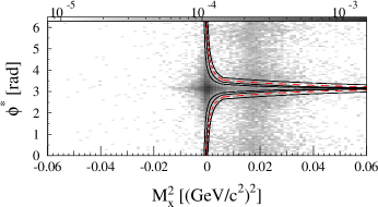
Figure 16: (color online) Radiative rejection overlay for lowest $\cos{\theta^{\,\ast}}$ bin. Several variations on the nominal rejection curves are displayed. The dashed curves are those using the nominal parameters.

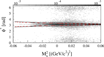
Figure 17: (color online) Radiative rejection overlay for intermediate and large $\cos{\theta^{\,\ast}}$ bin. Several variations on the nominal rejection curves are displayed. The dashed curves are those using the nominal parameters.

The errors due to the uncertainty in these rejection cuts are in the range 0.35 - 2.8%, which are very similar to the uncertainties induced by the missing mass cuts.

VII Extraction of Multipoles

In Eq. 7, the $\phi^{\,\ast}$ dependence of the differential cross section is explicit, but the $\cos{\theta^{\,\ast}}$ dependence is not so easily constrained unless one restricts oneself to states of definite angular momentum or at least states with some finite and small set of definite angular momentum contributions.

An empirical fitting procedure is used to extract information about the P₃₃ or $\Delta(1232)$ resonance in the present work. Multipole amplitudes of the Chew-Goldberger-Low-Nambu (CGLN Chew et al. (1957)) type: $E_{l\pm}$, $M_{l\pm}$ and $S_{l\pm}$ were extracted where $l$ is the orbital angular momentum of the final state and the final state nucleon spin is denoted by $\pm$. The procedure hinges on assuming a dominant magnetic dipole, $M_{1+}$, amplitude and assuming that one has only s- and p-wave contributions to the differential cross section.

VII.1 Expansion with s- and p-waves

The working assumption for the empirical fit is that in the partial wave series expansion only s- and p-waves will contribute. Indeed, the $\Delta(1232)$ resonance is a p-wave resonance, P₃₃ in spectroscopic notation. The next higher excitation, the P${}_{11}(1440)$, or “Roper” resonance is also p-wave. The lowest lying excitation which decays into a d-wave is the D${}_{13}(1520)$. Furthermore, the underlying non-resonant backgrounds are believed to be s- and p-wave dominated at these low excitation energies.

Thus, the $\cos{\theta^{\,\ast}}$ dependent cross sections can be written explicitly and fit to experimental data. The dependence that one obtains by including only the lowest two final state pion angular momentum contributions is well known Drechsel and Tiator (1992); Frolov (1998). It is then possible to write the s- and p-wave expansion in terms of three unknown functions which depend on $W$ and $Q^{2}$ and are well defined functions of $\cos{\theta^{\,\ast}}$ but not functions of $\phi^{\,\ast}$.

$$\frac{d\sigma^{\gamma^{\ast}}}{d\Omega^{\,\ast}_{\pi}}= A(\cos{\theta^{\,\ast}})+\epsilon B(\cos{\theta^{\,\ast}})\cos{2\phi^{\,\ast}}$$ (27)

$$+\sqrt{2\epsilon(1+\epsilon)}C(\cos{\theta^{\,\ast}})\cos{\phi^{\,\ast}}$$

The $\sigma_{L}$ and $\sigma_{T}$ contributions get combined into one parameter, $A$, since the present experiment does not vary $\epsilon$ at a fixed value of $Q^{2}$ and therefore cannot separate these contributions. Using the truncated partial wave expansion one can then write the explicit angular dependence.

$$A(\cos{\theta^{\,\ast}}) \equiv A_{0}+A_{1}\cos{\theta^{\,\ast}}+A_{2}\cos^{2}{\theta^{\,\ast}}$$ (28)

$$B(\cos{\theta^{\,\ast}}) \equiv B_{0}\sin^{2}{\theta^{\,\ast}}$$

$$C(\cos{\theta^{\,\ast}}) \equiv(C_{0}+C_{1}\cos{\theta^{\,\ast}})\sin{\theta^{\,\ast}}$$

The parameters $A_{i}$, $B_{i}$, and $C_{i}$ are now only functions of the electron variables $W$ and $Q^{2}$, and not functions of the hadronic center of mass angles. A simple way to proceed in characterizing the extracted cross sections is to fit the angular distributions in each $W$ and $Q^{2}$ bin independently. This point of view is taken in this section, since to include the $W$ and $Q^{2}$ dependence in the fitting procedures requires detailed knowledge of the dynamics at least at a level where one can add many resonance and background contributions with enough free parameters to obtain a physically realistic parameterization. Figure 18 shows an example of fit results using the $Q^{2}=$ 6.4 (GeV/c²)² experimental data and the $W=1.192,1.232$ and $1.272$ GeV center of mass energy bins. The previously described fit is superimposed onto the data.

Figure 18: Fit to differential cross sections at $W=1.192,1.232$ and $1.272$ GeV with $Q^{2}=6.43,6.36$ and $6.29$ (GeV/c²)² respectively. The data is binned in $\phi^{\,\ast}$ and displayed as a function of $\cos{\theta^{\,\ast}}$. Outer error bars are systematic. The values of $\chi^{2}/n_{dof}$ for these fits are 1.31, 0.79 and 1.46 respectively.

Figure 19: Fit to differential cross sections at $W=1.192,1.232$ and $1.272$ GeV with $Q^{2}=6.43,6.36$ and $6.29$ (GeV/c²)² respectively. The data is binned in $\cos{\theta^{\,\ast}}$ and displayed as a function of $\phi^{\,\ast}$. Outer error bars are systematic. The values of $\chi^{2}/n_{dof}$ for these fits are 1.31, 0.79 and 1.46 respectively.

This illustrates the procedure for energy independent analysis of the differential cross sections. The binning represented in Fig.18 shows 40 MeV wide W bins centered on $W=1.192,1.232$ and $1.272$ GeV along with ten angular bins in $\cos{\theta^{\,\ast}}$ and $\phi^{\,\ast}$. Since the measurement is unpolarized one should observe only symmetric distributions in $\phi^{\,\ast}$.

Figure 19 displays data points which are (to within statistical accuracy) symmetric about the point $\phi^{\,\ast}=\pi$. This fact is a good check on any extracted cross section. The $\phi^{\,\ast}$ symmetry is a general feature of the cross section data for the present experiment.

All of the other experimental observables can be extracted from these types of fits by assigning certain physical significance to the fit parameters. The extracted cross sections will be made available through Jefferson Lab for various world data fits or other scientific purposes. The extracted cross sections are also displayed in Tbls. LABEL:T:xntabl and LABEL:T:xntabh in the Appendix.

VII.2 Multipole Fitting

The fit parameters used in the last section had but one assumption in their use, namely, that they included only up to p-wave contributions. The $\chi^{2}$ parameters for these fits are fairly good and therefore one has confidence for at least the low $Q^{2}$ settings that s-wave and p-wave contributions approximate the cross section well.

One can now attempt to go further in the interpretation of these parameters by constraining the CGLN multipoles. The $M1$ dominance procedure Lyth (1978); Frolov (1998) has traditionally been employed to reduce the number of contributing multipoles in the s- and p-wave amplitudes so that they can be extracted from fits to the angular distributions. If one assumes that the $M_{1+}$ multipole dominates, the s- and p-wave fit parameters can be related to the multipole ratios in a simple way.

$$A_{0} =\frac{2W|\mathbf{k}^{\,\ast}_{\pi}|}{W^{2}-m_{p}^{2}}|M_{1+}|^{2}\left[\frac{5}{2}-3\frac{\Re\left(E_{1+}^{\ast}M_{1+}\right)}{|M_{1+}|^{2}}+\frac{\Re\left(M_{1+}^{\ast}M_{1-}\right)}{|M_{1+}|^{2}}\right]$$ (29)

$$A_{1} =\frac{2W|\mathbf{k}^{\,\ast}_{\pi}|}{W^{2}-m_{p}^{2}}|M_{1+}|^{2}2\frac{\Re\left(E_{0+}^{\ast}M_{1+}\right)}{|M_{1+}|^{2}}$$

$$A_{2} =\frac{2W|\mathbf{k}^{\,\ast}_{\pi}|}{W^{2}-m_{p}^{2}}|M_{1+}|^{2}\left[-\frac{3}{2}+9\frac{\Re\left(E_{1+}^{\ast}M_{1+}\right)}{|M_{1+}|^{2}}-3\frac{\Re\left(M_{1-}^{\ast}M_{1+}\right)}{|M_{1+}|^{2}}\right]$$

$$B_{0} =\frac{2W|\mathbf{k}^{\,\ast}_{\pi}|}{W^{2}-m_{p}^{2}}|M_{1+}|^{2}\left[-\frac{3}{2}-3\frac{\Re\left(E_{1+}^{\ast}M_{1+}\right)}{|M_{1+}|^{2}}-3\frac{\Re\left(M_{1-}^{\ast}M_{1+}\right)}{|M_{1+}|^{2}}\right]$$

$$C_{0} =\frac{2W|\mathbf{k}^{\,\ast}_{\pi}|}{W^{2}-m_{p}^{2}}|M_{1+}|^{2}\sqrt{\frac{2Q^{2}}{|\mathbf{q}^{\ast}|^{2}}}\frac{\Re\left(S_{0+}^{\ast}M_{1+}\right)}{|M_{1+}|^{2}}$$

$$C_{1} =\frac{2W|\mathbf{k}^{\,\ast}_{\pi}|}{W^{2}-m_{p}^{2}}|M_{1+}|^{2}6\sqrt{\frac{2Q^{2}}{|\mathbf{q}^{\ast}|^{2}}}\frac{\Re\left(S_{1+}^{\ast}M_{1+}\right)}{|M_{1+}|^{2}}$$

In Eq. 29, $\mathbf{k}^{\,\ast}_{\pi}$ is the pion momentum in the center of mass, $\mathbf{q}^{\,\ast}$ is the virtual photon momentum in the center of mass and $m_{p}$ is the proton rest mass. There are six combinations of multipoles, all involving $M_{1+}$. By substitution for the six parameters in Eq. 27 the differential cross section can be expressed in terms of the leading $|M_{1+}|^{2}$ and the five interference terms in Eq. 29. Then, the experimental differential cross sections can be fit to extract these six multipole combinations.

The results of the $W$-independent fits for the current experimental data sets are shown in Figs. 20 and 21.

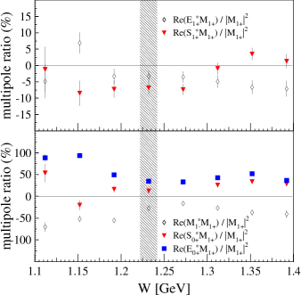
Figure 20: (color online) Results of the simple $M_{1+}$ dominance fit for the nominal $Q^{2}=$ 6.4 (GeV/c²)² data set as a function of invariant energy $W$. The region of the $\Delta(1232)$ resonance is shaded.

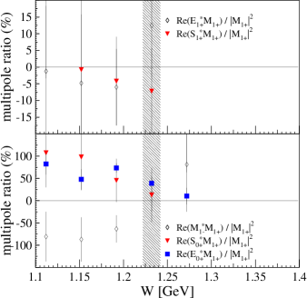
Figure 21: (color online) Results of the simple $M_{1+}$ dominance fit for the nominal $Q^{2}=$ 7.7 (GeV/c²)² data set as a function of invariant energy $W$. The region of the $\Delta(1232)$ resonance is shaded.

From Fig. 20 it is seen that even near the $\Delta(1232)$, unlike the situation for low $Q^{2}$, the assumption of $M_{1+}$ dominance is only approximate. This is due to a combination of factors. The $\Delta$ resonance is known to fall off with $Q^{2}$ more steeply than other resonances and background. The amplitudes of the Roper (P${}_{11}(1440)$) resonance, while very small at low $Q^{2}$ have recently been shown to become large Aznauryan et al. (2005) with increasing $Q^{2}$. These phenomena are manifested in the relative importance of $\Re\left(M_{1-}^{\ast}M_{1+}\right)/|M_{1+}|^{2}$ and $\Re\left(E_{0+}^{\ast}M_{1+}\right)/|M_{1+}|^{2}$ in Fig. 20.

The values of $R_{EM}$ and $R_{SM}$ extracted at the $W=1.232$ GeV and $Q^{2}=6.4$ (GeV/c²)² are listed in Tbl. 7. This includes systematic errors in the extracted multipole parameters. These are extracted with similar methods to those presented in Sec. VII.3. The values of $R_{EM}$, modulo the caveats given above, are somewhat consistent with previous values which are negative and small in magnitude. The value of $R_{SM}$ is more controversial. Previous analyses of the world data by two different schemes, JINR Aznauryan et al. (2005) and MAID Drechsel et al. (1999) yield differences of a factor of two.

As seen in Fig. 21 the fits for multipole amplitudes at the higher $Q^{2}$ ($W=1.232$ GeV, $Q^{2}=7.7$ (GeV/c²)²) are poorly constrained, since this data has less statistical significance and poor angular coverage. One can only say that it is likely that $R_{EM}$ continues to be small.

The angular integrals, $\sigma$, of the differential cross sections $d\sigma^{\gamma^{\ast}}/d\Omega^{\,\ast}_{\pi}$ were calculated in terms of the fit parameters. The errors on the fit parameters can then be propagated through to this integrated cross section. This method is the most consistent way of displaying the desired cross sections with the detector acceptance effects removed. The method is subject to large uncertainty when the data points have incomplete angular distribution. For the present data set this happens for the high $W$ points at higher $Q^{2}$.

Figures 22 and 23 display the experimentally observed angle-integrated cross sections and fits to them. For these figures the differential cross section with 16 $W$ bins and 49 angular bins were fit using the previous parameters. The angular bins included 7 $\phi^{\,\ast}$ bins and 7 $\cos{\theta^{\,\ast}}$ bins. The fits to the $W$ behavior include a resonance contribution with the appropriate threshold behavior Stoler (1993) and a polynomial background of various order. The specific function used to fit the resonance and background was the following:

$$\sigma =\frac{fa_{0}^{2}}{(W^{2}-a_{1}^{2})^{2}+a_{2}^{2}}+p(W-W_{th},\{a_{n}\}_{3}^{N})$$ (30)

$$f \equiv\sqrt{\left(\frac{W^{2}+m_{\pi}^{2}-m_{p}^{2}}{2W}\right)^{2}-m_{\pi}^{2}}.$$

The $a_{i}$ are adjustable parameters and the function $p(W-W_{th},\{a_{i}\}_{3}^{N})$ represents a polynomial in $W$ with $N-3$ terms. To obtain the best fit a polynomial including all non-zero integer and half-integer powers up to $(W-W_{th})$ was included in Fig. 22. For Fig. 23 the same polynomial was used. One can see that the background contribution is roughly 50% and 100% of the peak height for the lower $Q^{2}$ and higher $Q^{2}$ data respectively. One should be aware that this rough determination of the background has large systematic error due to the arbitrary selection of the type of polynomial to use. These factors can be used as a rough correction factor to the cross section for extraction of $(G_{M}^{\ast})^{2}$. The seemingly large background contribution for the higher $Q^{2}$ data indicates that the resonance may not be dominating the cross section at these high values of momentum transfer. The fit is a very rough approximation and detailed procedures with more physical inspiration are discussed at the end of this section.

Figure 22: The total angle-integrated cross section with $Q^{2}\sim$ 6.4 (GeV/c²)² at the $\Delta$ peak. Cross sections are fit with a Breit-Wigner function and a fractional power polynomial of first order.

Figure 23: The total angle-integrated cross section with $Q^{2}\sim$ 7.7 (GeV/c²)² at the $\Delta$ peak. Cross sections are fit with a Breit-Wigner function and a fractional power polynomial of first order. The dark inverted triangle data points are the only ones used to constrain the fit due to lack of statistics for higher $W$ and the possibility of small elastic radiative contamination at lower $W$.

We extracted the transition form factor $G_{M}^{\ast}$ from the angle integrated cross sections evaluated at the $\Delta$ pole position. The notation which we adopt is that of Jones and Scadron Jones and Scadron (1973) which is based on relativistic current structures in analogy with elastic scattering.

The magnetic form factor $G_{M}^{\ast}$ will be extractable and directly related to the multipole $M_{1+}$ if the resonance is completely dominant at the peak position. First note that when one integrates the angular distribution quoted in Eq. 27 one obtains $\frac{2}{3}(A_{2}+3A_{0})$. This expression can easily be put in terms of the multipole amplitudes (assuming, still, $M_{1+}$ dominance) to get:

$$\sigma=8\pi\frac{2W|\mathbf{k}^{\,\ast}_{\pi}|}{W^{2}-m_{p}^{2}}|M_{1+}|^{2}$$ (31)

One can therefore extract the (presumed dominant) $M_{1+}$ multipole from just a measure of the angle integrated cross section. Further, one has the relation:

$$\Im\left(M_{1+}^{(3/2)}\right)=\eta_{b}\sqrt{\frac{2}{3}}G_{M}^{\ast}.$$

The factor $\eta_{b}$ serves to relate the magnetic transition form factor to the multipole amplitude as in Ref. Burkert and Lee (2004). Therefore a measurement of the cross section, armed with the assumption that $M_{1+}\simeq i\Im\left(M_{1+}^{(3/2)}\right)$, is a direct measurement of the magnetic transition form factor assuming resonance and magnetic multipole dominance.

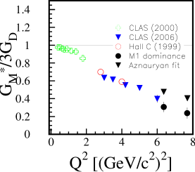
Figure 24: (color online) Current experimental situation for $G_{M}^{\ast}$ (in the Jones and Scadron convention) with increasing $Q^{2}$. The points are from CLAS Joo et al. (2002); Aznauryan et al. (2005); Ungaro et al. (2006), and Hall C Frolov et al. (1999). The error bars for the $M1$ dominance results are the sum (in quadrature) of the statistical and systematic errors. The result from the Aznauryan fit to the present cross section is also shown Aznauryan (2003) with only statistical error bars displayed.

Figure 24 shows the current experimental situation for the transition form factor including the values extracted in this work. The values for $G_{M}^{\ast}$ are computed by taking the total center of mass cross section at the $\Delta$ pole position ($W=$ 1.232 GeV) from Figs. 20 and 21 and correcting the resonance value using the fits displayed in Figs. 22 and 23. According to these fits the non-resonant background accounts for 50 % and 100 % of the resonant contribution for the $Q^{2}=$ 6.4 and 7.7 (GeV/c²)² points respectively. Note that these values are statistically quite well constrained by the data even at the higher $Q^{2}$ point. The results for $G_{M}^{\ast}$ are compared to the dipole form factor $G_{D}=3(1+Q^{2}/0.7)^{-2}$ in Fig. 24.

Clearly, although the transition form factor is well constrained statistically, the magnetic multipole dominance is a rather crude approximation since the total cross section is not simply due to the $M_{1+}$. The problem is that we have neglected all other amplitudes which do not interfere with $M_{1+}$, such as $|E_{0+}|^{2}$ and $|M_{1-}|^{2}$ which certainly contribute significantly to the total cross section, and should be included in the fit, especially at these higher values of $Q^{2}$. The numerical results of the fit for $G_{M}^{\ast}$ are given in Tbl. 7. The systematic uncertainties in $G_{M}^{\ast}$ introduced by this method have been quantified by obtaining $G_{M}^{\ast}$ for various assumptions of the background shape, and are significantly greater that the statistical uncertainties.

$Q^{2}$	$G_{M}^{\ast}/3G_{D}$	$R_{EM}$(%)	$R_{SM}$(%)
6.36	0.307 $\pm$ 0.0033 $\pm$0.058	-3.349 $\pm$1.711 $\pm$0.028	-6.894 $\pm$1.876 $\pm$0.084
7.69	0.238 $\pm$0.014 $\pm$0.059	12.482 $\pm$15.738 $\pm$0.056	-7.217 $\pm$12.819 $\pm$0.020

Table 7: The results of the fits to the data as described above. The first error is statistical, the second systematic.

A more realistic fitting procedure has been undertaken at Jefferson Lab. The analysis uses a unitary isobar model including appropriate non-resonant background contributions. The standard isobar approach of Drechsel et al. Drechsel et al. (1999) is complimented by the approach of Aznauryan Aznauryan (2003). The non-resonant background consists of Born and t-channel $\rho$ and $\omega$ contributions. The most up-to-date world data on nucleon-pion form factors and higher energy resonance contributions is used as well. The procedure is the same as was used to extract the $\Delta$ excitation parameters in Ref. Ungaro et al. (2006). Table 8 displays the relevant parameters and the errors.

$Q^{2}$	$G_{M}^{\ast}/3G_{D}$	$R_{EM}$(%)	$R_{SM}$(%)
6.36	0.477 $\pm$ 0.009 $\pm$0.043	-1.7 $\pm$1.9 $\pm$1.6	-22.3 $\pm$4.4 $\pm$3.4
7.69	0.404 $\pm$0.024 $\pm$0.056	-	-

Table 8: The results of the Jefferson Lab fitting procedure carried out by Aznauryan. The first error is statistical, the second systematic.

VII.3 Systematic Errors in Extracted Amplitudes

One may also be interested in the systematic error on an observable extracted by a fitting method. Figure 25 shows how our estimator for $R_{EM}$ varies due to the missing mass restriction.

Figure 25: The variation of the $R_{EM}$ estimator on missing mass restriction. From left to right the restrictions are labeled from narrowest to widest with the arrow marking the nominal. The widths which correspond to this plot are displayed in Fig. 15.

An estimate for the uncertainty on $R_{EM}$ due to the missing mass restriction is 1.0%, based on this analysis. The systematic errors on the other extracted multipoles are evaluated in the same way.

VIII Results in the Context of Previous World Data

Contributions to the previous world data which are noted here are the following. At lower $Q^{2}$ data have been obtained by the MAMI (Mainzer Microtron) Pospischil et al. (2001); Ahrens et al. (2004); Elsner et al. (2006); Stave et al. (2006); Sparveris et al. (2007), ELSA (University of Bonn) Bantes (2003), LEGS (Brookhaven) collaboration Sandorfi et al. (1998); Blanpied et al. (1997) and the BATES (MIT) collaboration Sparveris et al. (2005). The Jefferson Laboratory spectrometer Hall A Kelly et al. (2005) has also made a significant contribution to the question of the structure of the $N\rightarrow\Delta$ transition. CLAS (Jefferson Laboratory) has also obtained a large amount of data over a large range in $Q^{2}$ Joo et al. (2002); Aznauryan et al. (2005); Ungaro et al. (2006). Jefferson Laboratory Hall C Frolov et al. (1999), at $Q^{2}=2.8$ and $4.0$ (GeV/c²)² was the predecessor to the present experiment.

VIII.1 The Electric Quadrupole to Magnetic Dipole ratio $R_{EM}$

Figure 26 shows the status of the world data on $R_{EM}$, including the present result obtained by the M1 dominance method and the more sophisticated Jefferson Lab (Aznauryan) fit. The real photon point at $Q^{2}=0$ is small in magnitude and negative in sign. This situation shows no drastic change up to $Q^{2}$ of about 7.7 (GeV/c²)².

The results for $R_{EM}$ indicate that the baryon helicity non-conserving element is on the order of two times as great as the baryon helicity conserving element. Perturbative QCD predicts that the helicity non-conserving element vanishes, causing $R_{EM}\rightarrow 1$ Brodsky and Lepage (1981); Carlson (1986). In the realm of our simplified multipole extraction procedure and also that of a unitary isobar fit, one therefore finds that the data indicates the pQCD limit has not yet been reached for $\Delta$ excitation.

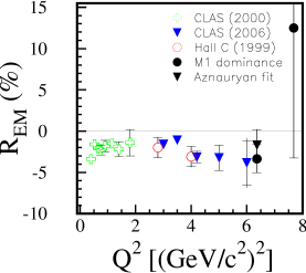
Figure 26: (color online) Current experimental situation for $R_{EM}$ with increasing $Q^{2}$. The points are from CLAS Joo et al. (2002); Aznauryan et al. (2005); Ungaro et al. (2006), and Hall C Frolov et al. (1999). The outer error bars for the $M1$ dominance results are the sum (in quadrature) of the statistical and systematic errors. The result from the Aznauryan fit to the present cross section is also shown Aznauryan (2003) with only statistical error bars displayed.

VIII.2 Magnetic Form Factor $G_{M}^{\ast}$

Figure 24 shows the status of the world data on $G_{M}^{\ast}$ relative to the dipole form factor $G_{D}=3(1+Q^{2}/0.7)^{-2}$. For the present data the result is obtained by the methods discussed in Sec. VII.2. At lower $Q^{2}$ the resonance is quite strong and the $M_{1+}$ multipole dominates neutral pion production in the vicinity of the $\Delta$ resonance pole, so that $G_{M}^{\ast}$ form factors which have been extracted by a variety of approaches yield rather similar results. However, at high $Q^{2}$ the rapid decay of $G_{M}^{\ast}$ relative to the non-resonant background, and relative to the increased importance of the tails of other resonances, such as the P${}_{11}(1440)$ (Roper) resonance requires one to make a careful analysis in the framework of all the available data. This has been the goal of several analysis groups including MAID, SAID and JINR.

Overall, $G_{M}^{\ast}$ is falling much faster than the dipole form factor $G_{D}$ in the previously measured $Q^{2}$ region from 0 to 5 or 6 (GeV/c²)². Asymptotically, if the pQCD constituent scaling rules were operative, this form factor should begin to scale as $1/Q^{4}$, as the dipole form factor does, so the constituent scaling does not yet occur for $G_{M}^{\ast}$. This is consistent with the result for $R_{EM}$. The helicity non-conserving amplitude should dominate $G_{M}^{\ast}$ whenever $R_{EM}$ is small. Thus, the data on $G_{M}^{\ast}$ and $R_{EM}$ are consistent. One may then speculate that when $R_{EM}$ becomes large and positive, the $G_{M}^{\ast}$ may begin to scale. For completeness, the current experimental situation for $R_{SM}$ is shown in Fig. 27. It seems that the M1 dominance extraction procedure used here is especially questionable in the case of $R_{SM}$ but the Jefferson Lab procedure yeilds results which are consistent with previously extracted values at lower $Q^{2}$.

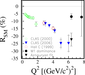
Figure 27: (color online) Current experimental situation for $R_{SM}$ with increasing $Q^{2}$. The points are from CLAS Joo et al. (2002); Aznauryan et al. (2005); Ungaro et al. (2006), and Hall C Frolov et al. (1999). The outer error bars for the $M1$ dominance results are the sum (in quadrature) of the statistical and systematic errors. The result from the Aznauryan fit to the present cross section is also shown Aznauryan (2003) with only statistical error bars displayed.

IX Conclusion

This work has accomplished several goals. The first and foremost goal was to extract the center of mass neutral pion electroproduction cross section in the invariant mass region roughly corresponding to the well-known $\Delta$ resonance. This goal was accomplished and the systematic errors on the cross section were evaluated using the best current knowledge of the detector systems and analysis procedures. The next goal of the analysis was to investigate (in a simplified way) what the cross sections suggest for the most important multipole amplitudes and transition form factors relating to the measured process and in particular to the $\Delta$ resonance.

In the realm of a fit which includes only s-wave and p-wave contributions and assumes that the multipole $M_{1+}$ dominates all other multipoles (an assumption which seems to be challenged by the size of $E_{0+}$), with the $\Delta$ resonance being dominant at the resonance position, one can obtain values for $R_{EM}$, $R_{SM}$ and $G_{M}^{\ast}$. The specifications of $R_{EM}$ and $R_{SM}$ depend in detail on the angular distribution of the cross section and thus are only well determined for the $Q^{2}=6.4$ (GeV/c²)² data set. The most significant facts that are obtained using these methods are that $R_{EM}=-3.3\pm 1.7$% and that $G_{M}^{\ast}$ seems to be still dropping much faster than the simple dipole form, suggesting that there are soft mechanisms in the $\Delta$ excitation which are still important Carlson and Mukhopadhyay (1998).

It is important to reiterate the physical effects which were not considered in this work. Everything assumes that single photon exchange is completely appropriate for dealing with observables measured to the accuracy that was displayed in this data. This is probably a good assumption but there are some places, including calculation of radiative effects which two photon exchange mechanisms might have a more important role. These are left to subsequent study. There has been some recent work on the subject and it is hopeful that the two photon effects can be understood in detail and corrected for in the future if necessary Pascalutsa et al. (2006). In extracting our estimates for the multipole ratios and transition form factor of the $\Delta$ excitations it was assumed that the $\Delta$ dominates at the resonance position, though this assumption has already been shown to be suspect in Sec. VII.2. Contributions from multipoles other than $M_{1+}$, specifically $E_{0+}$ may also be showing their importance and thus spoiling the M1 dominance that was assumed.

The more physically motivated fitting procedure explored produced results for $G_{M}^{\ast}$ and $R_{EM}$ which were consistent with the interpretations from the simpler M1 dominance procedure. Specific values for these parameters are modified in this procedure and, in particular, $R_{EM}=-1.7\pm 1.9$% for $Q^{2}=6.4$ (GeV/c²)². $R_{SM}$ becomes much smaller than the M1 dominance result and this fact is not reproduced in other unitary isobar fitting procedures such as MAID currently.

These conclusions seem to indicate that the studied process is not in a regime where perturbative QCD is dominating behaviour. Continued investigation is necessary to help uncover the inner workings of hadronic physics and QCD, especially in this intermediate energy region between hadronic and quark descriptions.

As for measurements at higher $Q^{2}$, this will have to await the completion of the Jefferson Lab 12 GeV upgrade.

*

Appendix A Tables of Differential Cross Sections

The measured differential cross sections mentioned throughout the text are listed here. The author can be contacted for an electronic version of these data points.

Table 9: Differential cross sections for the small SOS spectrometer angle.

$Q^{2}$	$\epsilon$	$W$	$\cos{\theta^{\,\ast}}$	$\phi^{\,\ast}$	$d\sigma^{\gamma^{\ast}}$	$\sigma_{stat}$	$\sigma_{norm}$	$\sigma_{sys}$
(GeV2)	none	(GeV)	none	(rad)	(nb/Sr)	(nb/Sr)	(nb/Sr)	(nb/Sr)
6.564	0.4523	1.112	-0.9	-2.827	5.1456	3.8602	0.29671	0.0022301
6.564	0.4523	1.112	-0.9	-1.571	7.3159	5.1838	0.42185	0.00092151
6.564	0.4523	1.112	-0.9	-0.9425	4.721	3.3702	0.27223	0.0081633
6.564	0.4523	1.112	-0.9	-0.3142	6.7928	6.7933	0.39169	0.0002199
6.564	0.4523	1.112	-0.9	0.3142	4.2895	4.2898	0.24734	0.0023096
6.564	0.4523	1.112	-0.9	0.9425	2.2098	2.2099	0.12742	0.0043183
6.564	0.4523	1.112	-0.9	1.571	2.2215	2.2216	0.1281	0.0026498
6.564	0.4523	1.112	-0.9	2.199	2.6294	2.6295	0.15162	0.0038613
6.564	0.4523	1.112	-0.7	-2.827	9.0972	6.964	0.52457	8.987e-06
6.564	0.4523	1.112	-0.7	-1.571	5.3862	3.8094	0.31059	0.0012255
6.564	0.4523	1.112	-0.7	-0.9425	3.0943	3.0944	0.17843	0.00088908
6.564	0.4523	1.112	-0.7	-0.3142	18.853	10.933	1.0871	0.0018922
6.564	0.4523	1.112	-0.7	0.3142	10.064	10.064	0.5803	0.0037097
6.564	0.4523	1.112	-0.7	0.9425	3.1474	3.1475	0.18149	0.0027893
6.564	0.4523	1.112	-0.7	1.571	4.9941	3.6308	0.28798	0.00041656
6.564	0.4523	1.112	-0.7	2.199	5.2545	3.7235	0.30299	0.0012938
6.564	0.4523	1.112	-0.5	-2.827	6.9861	5.0843	0.40284	0.00013218
6.564	0.4523	1.112	-0.5	-2.199	5.2735	3.7522	0.30408	0.0015351
6.564	0.4523	1.112	-0.5	-1.571	15.133	9.2937	0.87261	0.00040333
6.564	0.4523	1.112	-0.5	-0.9425	3.8679	3.8681	0.22303	0.00025298
6.564	0.4523	1.112	-0.5	-0.3142	9.3756	6.6308	0.54062	0.0015795
6.564	0.4523	1.112	-0.5	0.3142	25.968	13.199	1.4974	0.0024584
6.564	0.4523	1.112	-0.5	0.9425	6.8284	3.9439	0.39375	0.00024808
6.564	0.4523	1.112	-0.5	1.571	3.7445	2.6479	0.21592	0.00048817
6.564	0.4523	1.112	-0.5	2.199	10.019	5.0939	0.5777	0.00022567
6.564	0.4523	1.112	-0.5	2.827	2.2994	2.2995	0.13259	0.00096042
6.564	0.4523	1.112	-0.3	-2.827	2.1049	2.105	0.12138	0.00022043
6.564	0.4523	1.112	-0.3	-2.199	2.1232	2.1233	0.12243	0.00066444
6.564	0.4523	1.112	-0.3	-1.571	5.0376	3.6624	0.29048	0.00023
6.564	0.4523	1.112	-0.3	-0.9425	11.234	5.759	0.6478	0.0015196
6.564	0.4523	1.112	-0.3	-0.3142	57.944	37.256	3.3412	0.023004
6.564	0.4523	1.112	-0.3	0.3142	60.951	37.025	3.5146	0.015764
6.564	0.4523	1.112	-0.3	1.571	4.2344	3.0186	0.24417	1.9907e-05
6.564	0.4523	1.112	-0.3	2.199	8.5962	5.8576	0.49568	0.00070534
6.564	0.4523	1.112	-0.3	2.827	10.139	4.5686	0.58464	0.00037001
6.564	0.4523	1.112	-0.1	-2.827	21.981	18.924	1.2675	0.00044294
6.564	0.4523	1.112	-0.1	-2.199	15.078	6.4268	0.86942	0.00046145
6.564	0.4523	1.112	-0.1	-0.9425	7.9584	5.628	0.45891	0.00028018
6.564	0.4523	1.112	-0.1	-0.3142	12.381	7.4374	0.71391	0.0060386
6.564	0.4523	1.112	-0.1	0.3142	38.655	14.038	2.2289	0.012986
6.564	0.4523	1.112	-0.1	0.9425	32.695	11.241	1.8853	0.00096376
6.564	0.4523	1.112	-0.1	1.571	5.07	3.6534	0.29235	0.00045379
6.564	0.4523	1.112	-0.1	2.199	16.158	6.9458	0.93172	2.4304e-05
6.564	0.4523	1.112	-0.1	2.827	17.923	7.5007	1.0335	0.00013431
6.564	0.4523	1.112	0.1	-2.827	12.606	5.3866	0.72692	0.00038193
6.564	0.4523	1.112	0.1	-2.199	33.452	11.706	1.929	0.00028722
6.564	0.4523	1.112	0.1	-1.571	10.135	5.1739	0.58443	4.7344e-05
6.564	0.4523	1.112	0.1	-0.9425	16.65	7.618	0.96009	0.001648
6.564	0.4523	1.112	0.1	-0.3142	14.395	7.2267	0.83003	0.00039035
6.564	0.4523	1.112	0.1	0.3142	11.853	8.3824	0.68346	0.002947
6.564	0.4523	1.112	0.1	0.9425	13.464	6.896	0.77635	0.0033774
6.564	0.4523	1.112	0.1	1.571	7.8324	4.5961	0.45164	0.00061512
6.564	0.4523	1.112	0.1	2.199	13.884	7.775	0.8006	0.00046377
6.564	0.4523	1.112	0.1	2.827	13.592	7.157	0.78377	0.0008163
6.564	0.4523	1.112	0.3	-2.827	21.274	10.254	1.2267	0.0014908
6.564	0.4523	1.112	0.3	-2.199	22.01	8.9387	1.2692	0.00044372
6.564	0.4523	1.112	0.3	-1.571	10.256	8.349	0.59136	0.00027807
6.564	0.4523	1.112	0.3	-0.9425	22.719	9.5587	1.3101	0.00095757
6.564	0.4523	1.112	0.3	-0.3142	30.273	12.796	1.7456	0.0019359
6.564	0.4523	1.112	0.3	0.3142	22.619	10.449	1.3043	0.0038453
6.564	0.4523	1.112	0.3	0.9425	18.643	7.0854	1.075	0.00021287
6.564	0.4523	1.112	0.3	1.571	14.325	7.9453	0.82605	0.00039282
6.564	0.4523	1.112	0.3	2.199	26.943	9.883	1.5536	0.00059145
6.564	0.4523	1.112	0.3	2.827	20.418	8.815	1.1774	0.00065767
6.564	0.4523	1.112	0.5	-2.827	25.383	14.271	1.4637	0.00051841
6.564	0.4523	1.112	0.5	-2.199	23.745	8.197	1.3692	0.00017216
6.564	0.4523	1.112	0.5	-1.571	32.625	22.218	1.8813	0.003919
6.564	0.4523	1.112	0.5	-0.9425	37.605	17.136	2.1684	0.0028012
6.564	0.4523	1.112	0.5	-0.3142	36.006	13.992	2.0762	0.0039868
6.564	0.4523	1.112	0.5	0.3142	27.442	12.417	1.5824	0.0039036
6.564	0.4523	1.112	0.5	0.9425	14.804	6.7183	0.85365	0.00037035
6.564	0.4523	1.112	0.5	1.571	43.139	17.449	2.4875	0.0012527
6.564	0.4523	1.112	0.5	2.199	14.845	6.3257	0.85603	1.5783e-05
6.564	0.4523	1.112	0.5	2.827	29.616	13.283	1.7077	0.00040822
6.564	0.4523	1.112	0.7	-2.827	11.805	5.4659	0.68069	0.0012519
6.564	0.4523	1.112	0.7	-2.199	40.395	12.581	2.3293	1.9875e-05
6.564	0.4523	1.112	0.7	-1.571	23.678	10.283	1.3654	0.00098633
6.564	0.4523	1.112	0.7	-0.9425	12.714	7.4858	0.73313	0.0003508
6.564	0.4523	1.112	0.7	-0.3142	16.733	8.5071	0.96488	0.0010914
6.564	0.4523	1.112	0.7	0.3142	29.894	10.867	1.7238	0.0028034
6.564	0.4523	1.112	0.7	0.9425	13.33	6.0632	0.76863	0.00046927
6.564	0.4523	1.112	0.7	1.571	24.513	9.0204	1.4135	0.00025205
6.564	0.4523	1.112	0.7	2.199	36.248	15.719	2.0902	3.2103e-05
6.564	0.4523	1.112	0.7	2.827	56.462	22.827	3.2557	0.0028597
6.564	0.4523	1.112	0.9	-2.827	26.084	7.9836	1.5041	0.00010956
6.564	0.4523	1.112	0.9	-2.199	28.747	9.6291	1.6576	0.00050844
6.564	0.4523	1.112	0.9	-1.571	27.13	10.884	1.5644	0.00057601
6.564	0.4523	1.112	0.9	-0.9425	29.978	13.043	1.7286	0.0014522
6.564	0.4523	1.112	0.9	-0.3142	16.333	7.3186	0.94181	0.0034801
6.564	0.4523	1.112	0.9	0.3142	17.577	7.9139	1.0135	0.001574
6.564	0.4523	1.112	0.9	0.9425	22.467	8.2086	1.2955	0.00082809
6.564	0.4523	1.112	0.9	1.571	8.625	4.3782	0.49734	0.001486
6.564	0.4523	1.112	0.9	2.199	65.34	23.529	3.7677	0.00070848
6.564	0.4523	1.112	0.9	2.827	49.614	13.329	2.8609	0.00027116
6.5	0.45	1.152	-0.9	-2.827	18.145	6.9597	1.0463	0.0017944
6.5	0.45	1.152	-0.9	-2.199	6.0778	3.5869	0.35046	0.00249
6.5	0.45	1.152	-0.9	-1.571	26.717	9.6402	1.5406	0.0049899
6.5	0.45	1.152	-0.9	-0.9425	1.9034	1.9035	0.10976	0.0022291
6.5	0.45	1.152	-0.9	-0.3142	19.498	11.898	1.1243	0.0046318
6.5	0.45	1.152	-0.9	0.3142	11.033	6.3937	0.6362	0.0030675
6.5	0.45	1.152	-0.9	0.9425	9.2862	5.3746	0.53547	0.0024866
6.5	0.45	1.152	-0.9	1.571	18.096	7.0113	1.0435	0.0017757
6.5	0.45	1.152	-0.9	2.199	17.026	7.1308	0.98179	0.00083069
6.5	0.45	1.152	-0.7	-2.827	35.433	15.445	2.0432	0.0014057
6.5	0.45	1.152	-0.7	-2.199	13.571	5.5982	0.78253	0.0025068
6.5	0.45	1.152	-0.7	-1.571	13.082	5.8924	0.75437	0.00065575
6.5	0.45	1.152	-0.7	-0.9425	12.134	5.4747	0.69971	0.00075663
6.5	0.45	1.152	-0.7	-0.3142	6.9187	5.0035	0.39895	0.0024212
6.5	0.45	1.152	-0.7	0.3142	21.501	9.7855	1.2398	0.0020319
6.5	0.45	1.152	-0.7	0.9425	10.937	5.5517	0.63064	0.00021486
6.5	0.45	1.152	-0.7	1.571	15.875	6.1564	0.9154	0.00083043
6.5	0.45	1.152	-0.7	2.199	11.743	4.8013	0.67715	0.00080767
6.5	0.45	1.152	-0.7	2.827	1.9803	1.9804	0.11419	0.001676
6.5	0.45	1.152	-0.5	-2.827	8.0384	3.6342	0.46352	0.00031068
6.5	0.45	1.152	-0.5	-2.199	26.937	8.9194	1.5533	1.098e-05
6.5	0.45	1.152	-0.5	-1.571	16.887	6.0553	0.97376	0.00089984
6.5	0.45	1.152	-0.5	-0.9425	23.01	7.8875	1.3268	0.0012879
6.5	0.45	1.152	-0.5	-0.3142	10.717	6.1916	0.61795	0.0017522
6.5	0.45	1.152	-0.5	0.3142	46.007	15.642	2.6529	0.0017078
6.5	0.45	1.152	-0.5	0.9425	20.201	6.8789	1.1648	0.00118
6.5	0.45	1.152	-0.5	1.571	15.294	5.646	0.88189	0.00017736
6.5	0.45	1.152	-0.5	2.199	23.898	8.7182	1.378	1.9861e-05
6.5	0.45	1.152	-0.5	2.827	12.896	10.352	0.74359	0.00024213
6.5	0.45	1.152	-0.3	-2.827	23.739	6.7723	1.3689	0.00028304
6.5	0.45	1.152	-0.3	-2.199	12.511	4.8968	0.72144	0.0007588
6.5	0.45	1.152	-0.3	-1.571	20.064	6.5212	1.157	0.0021651
6.5	0.45	1.152	-0.3	-0.9425	18.918	6.8887	1.0909	0.0018553
6.5	0.45	1.152	-0.3	-0.3142	27.414	8.8345	1.5808	0.014441
6.5	0.45	1.152	-0.3	0.3142	42.518	12.234	2.4517	0.017976
6.5	0.45	1.152	-0.3	0.9425	20.871	7.1753	1.2035	0.00092685
6.5	0.45	1.152	-0.3	1.571	17.69	6.9128	1.02	0.0041457
6.5	0.45	1.152	-0.3	2.199	18.642	6.8938	1.0749	0.00027403
6.5	0.45	1.152	-0.3	2.827	19.092	7.0354	1.1009	6.3843e-06
6.5	0.45	1.152	-0.1	-2.827	14.411	5.2958	0.83096	0.0014044
6.5	0.45	1.152	-0.1	-2.199	20.98	6.6856	1.2098	0.00026931
6.5	0.45	1.152	-0.1	-1.571	16.894	6.0924	0.97413	0.00079208
6.5	0.45	1.152	-0.1	-0.9425	20.26	7.446	1.1682	0.00087771
6.5	0.45	1.152	-0.1	-0.3142	36.521	11.339	2.1059	0.0076459
6.5	0.45	1.152	-0.1	0.3142	11.814	5.3081	0.68124	0.0084097
6.5	0.45	1.152	-0.1	0.9425	3.8207	2.7026	0.22031	0.0016472
6.5	0.45	1.152	-0.1	1.571	14.694	5.3006	0.84727	0.0017377
6.5	0.45	1.152	-0.1	2.199	24.899	8.0518	1.4357	0.00012292
6.5	0.45	1.152	-0.1	2.827	30.757	8.5402	1.7736	0.0001201
6.5	0.45	1.152	0.1	-2.827	13.383	5.2515	0.77168	0.00017631
6.5	0.45	1.152	0.1	-2.199	41.686	11.285	2.4037	0.00017777
6.5	0.45	1.152	0.1	-1.571	14.612	5.2148	0.84254	0.00082403
6.5	0.45	1.152	0.1	-0.9425	9.2767	5.3739	0.53492	0.00049922
6.5	0.45	1.152	0.1	-0.3142	15.571	7.9025	0.89788	0.00088619
6.5	0.45	1.152	0.1	0.3142	18.741	7.3384	1.0807	0.0046192
6.5	0.45	1.152	0.1	0.9425	29.882	8.5191	1.7231	0.0017976
6.5	0.45	1.152	0.1	1.571	34.162	10.313	1.9699	0.00017074
6.5	0.45	1.152	0.1	2.199	22.97	6.6448	1.3245	0.0012701
6.5	0.45	1.152	0.1	2.827	43.99	12.208	2.5366	0.0010365
6.5	0.45	1.152	0.3	-2.827	31.647	9.0903	1.8249	0.00068702
6.5	0.45	1.152	0.3	-2.199	21.628	7.2699	1.2471	0.00074356
6.5	0.45	1.152	0.3	-1.571	19.847	8.7072	1.1444	0.00065724
6.5	0.45	1.152	0.3	-0.9425	24.887	8.6559	1.435	0.00049459
6.5	0.45	1.152	0.3	-0.3142	33.187	10.845	1.9136	0.0045404
6.5	0.45	1.152	0.3	0.3142	40.921	12.84	2.3596	0.0005751
6.5	0.45	1.152	0.3	0.9425	27.256	8.5396	1.5716	0.0010433
6.5	0.45	1.152	0.3	1.571	24.902	7.4202	1.4359	6.5783e-05
6.5	0.45	1.152	0.3	2.199	33.125	9.685	1.9101	0.00056281
6.5	0.45	1.152	0.3	2.827	32.453	9.8415	1.8713	0.002699
6.5	0.45	1.152	0.5	-2.827	27.459	8.0943	1.5834	0.00023543
6.5	0.45	1.152	0.5	-2.199	58.445	14.86	3.3701	0.00044593
6.5	0.45	1.152	0.5	-1.571	54.885	13.22	3.1648	7.9631e-05
6.5	0.45	1.152	0.5	-0.9425	34.496	8.9942	1.9892	0.00096374
6.5	0.45	1.152	0.5	-0.3142	41.01	13.169	2.3647	0.0010998
6.5	0.45	1.152	0.5	0.3142	62.484	16.608	3.603	0.0024983
6.5	0.45	1.152	0.5	0.9425	16.555	5.5869	0.95462	0.00034137
6.5	0.45	1.152	0.5	1.571	52.215	13.614	3.0109	0.00028911
6.5	0.45	1.152	0.5	2.199	34.57	9.6765	1.9934	0.0008153
6.5	0.45	1.152	0.5	2.827	36.942	11.728	2.1302	0.00093319
6.5	0.45	1.152	0.7	-2.827	47.139	10.703	2.7182	0.00037351
6.5	0.45	1.152	0.7	-2.199	42.466	10.207	2.4487	0.0036182
6.5	0.45	1.152	0.7	-1.571	33.824	9.7252	1.9504	0.0012732
6.5	0.45	1.152	0.7	-0.9425	22.934	6.5803	1.3225	0.00092187
6.5	0.45	1.152	0.7	-0.3142	32.298	10.145	1.8624	0.00084861
6.5	0.45	1.152	0.7	0.3142	29.56	9.2845	1.7045	0.0021726
6.5	0.45	1.152	0.7	0.9425	39.571	11.679	2.2818	0.00050139
6.5	0.45	1.152	0.7	1.571	46.772	12.078	2.697	0.0021948
6.5	0.45	1.152	0.7	2.199	38.138	10.43	2.1992	0.00013593
6.5	0.45	1.152	0.7	2.827	51.48	10.86	2.9685	0.00032478
6.5	0.45	1.152	0.9	-2.827	33.591	8.4682	1.9369	0.00074668
6.5	0.45	1.152	0.9	-2.199	46.989	11.545	2.7095	0.00093814
6.5	0.45	1.152	0.9	-1.571	45.695	9.9498	2.6349	0.0013404
6.5	0.45	1.152	0.9	-0.9425	76.266	20.674	4.3977	0.0010198
6.5	0.45	1.152	0.9	-0.3142	61.428	18.621	3.5421	0.00045233
6.5	0.45	1.152	0.9	0.3142	30.807	9.3346	1.7764	0.0011254
6.5	0.45	1.152	0.9	0.9425	60.824	14.202	3.5073	6.831e-05
6.5	0.45	1.152	0.9	1.571	40.541	9.8438	2.3377	0.0002841
6.5	0.45	1.152	0.9	2.199	44.425	9.6964	2.5617	4.4771e-05
6.5	0.45	1.152	0.9	2.827	70.344	20.238	4.0563	0.001191
6.432	0.4478	1.192	-0.9	-2.827	11.047	4.6631	0.63698	0.0017573
6.432	0.4478	1.192	-0.9	-2.199	24.648	6.9704	1.4213	0.0013357
6.432	0.4478	1.192	-0.9	-1.571	45.288	16.74	2.6115	0.0023814
6.432	0.4478	1.192	-0.9	-0.9425	42.322	9.851	2.4404	0.0015309
6.432	0.4478	1.192	-0.9	-0.3142	22.343	9.9233	1.2884	0.001362
6.432	0.4478	1.192	-0.9	0.3142	22.652	9.4033	1.3062	0.0019144
6.432	0.4478	1.192	-0.9	0.9425	18.813	6.1967	1.0848	0.0017846
6.432	0.4478	1.192	-0.9	1.571	24.661	7.3622	1.422	1.2567e-05
6.432	0.4478	1.192	-0.9	2.199	24.424	6.8611	1.4083	0.0002261
6.432	0.4478	1.192	-0.9	2.827	31.82	11.863	1.8348	0.0029783
6.432	0.4478	1.192	-0.7	-2.827	28.185	9.2268	1.6252	0.001725
6.432	0.4478	1.192	-0.7	-2.199	35.426	9.3556	2.0428	0.0019855
6.432	0.4478	1.192	-0.7	-1.571	29.784	8.1188	1.7174	0.0026646
6.432	0.4478	1.192	-0.7	-0.9425	55.417	12.542	3.1955	0.0083037
6.432	0.4478	1.192	-0.7	-0.3142	48.56	14.913	2.8001	0.003259
6.432	0.4478	1.192	-0.7	0.3142	50.004	15.059	2.8833	0.0053559
6.432	0.4478	1.192	-0.7	0.9425	26.731	7.896	1.5414	3.3419e-05
6.432	0.4478	1.192	-0.7	1.571	29.246	7.8775	1.6864	0.0010023
6.432	0.4478	1.192	-0.7	2.199	17.781	6.3649	1.0253	0.0019437
6.432	0.4478	1.192	-0.7	2.827	31.563	8.7715	1.82	0.00079598
6.432	0.4478	1.192	-0.5	-2.827	28.746	8.2293	1.6576	0.00084156
6.432	0.4478	1.192	-0.5	-2.199	39.526	11.852	2.2792	0.0001476
6.432	0.4478	1.192	-0.5	-1.571	43.261	17.984	2.4945	0.0023327
6.432	0.4478	1.192	-0.5	-0.9425	53.978	11.313	3.1125	0.0011343
6.432	0.4478	1.192	-0.5	-0.3142	51.655	13.837	2.9786	0.0010873
6.432	0.4478	1.192	-0.5	0.3142	54.787	14.796	3.1592	0.0019867
6.432	0.4478	1.192	-0.5	0.9425	54.459	11.06	3.1403	0.001325
6.432	0.4478	1.192	-0.5	1.571	37.297	13.053	2.1507	0.0010589
6.432	0.4478	1.192	-0.5	2.199	29.37	10.165	1.6935	0.00065385
6.432	0.4478	1.192	-0.5	2.827	27.495	6.1536	1.5854	0.0010455
6.432	0.4478	1.192	-0.3	-2.827	43.185	11.579	2.4901	0.001904
6.432	0.4478	1.192	-0.3	-2.199	38.691	10.822	2.231	0.0024219
6.432	0.4478	1.192	-0.3	-1.571	50.054	14.629	2.8862	0.0020117
6.432	0.4478	1.192	-0.3	-0.9425	63.103	12.934	3.6387	0.0026457
6.432	0.4478	1.192	-0.3	-0.3142	77.045	14.807	4.4427	0.018186
6.432	0.4478	1.192	-0.3	0.3142	74.528	15.104	4.2975	0.014635
6.432	0.4478	1.192	-0.3	0.9425	27.35	7.5086	1.5771	0.00083163
6.432	0.4478	1.192	-0.3	1.571	89.809	21.563	5.1786	0.001246
6.432	0.4478	1.192	-0.3	2.199	58.367	17.32	3.3656	0.0025915
6.432	0.4478	1.192	-0.3	2.827	37.457	8.4084	2.1599	4.4495e-05
6.432	0.4478	1.192	-0.1	-2.827	35.32	7.8296	2.0367	0.0002033
6.432	0.4478	1.192	-0.1	-2.199	59.419	14.124	3.4263	5.4025e-05
6.432	0.4478	1.192	-0.1	-1.571	34.666	9.183	1.9989	0.00044981
6.432	0.4478	1.192	-0.1	-0.9425	51.695	12.076	2.9809	0.0015011
6.432	0.4478	1.192	-0.1	-0.3142	95.15	26.268	5.4866	0.010962
6.432	0.4478	1.192	-0.1	0.3142	56.694	12.538	3.2691	0.0077864
6.432	0.4478	1.192	-0.1	0.9425	68.652	21.746	3.9586	0.0043344
6.432	0.4478	1.192	-0.1	1.571	35.836	9.3193	2.0664	0.0013248
6.432	0.4478	1.192	-0.1	2.199	43.109	10.151	2.4858	3.3311e-05
6.432	0.4478	1.192	-0.1	2.827	46.285	10.656	2.6689	0.0014317
6.432	0.4478	1.192	0.1	-2.827	79.955	17.092	4.6104	7.4407e-05
6.432	0.4478	1.192	0.1	-2.199	43.811	9.7757	2.5263	0.0010392
6.432	0.4478	1.192	0.1	-1.571	45.899	11.973	2.6467	0.001071
6.432	0.4478	1.192	0.1	-0.9425	55.775	11.93	3.2161	0.0014437
6.432	0.4478	1.192	0.1	-0.3142	62.749	14.164	3.6183	0.0017714
6.432	0.4478	1.192	0.1	0.3142	37.805	10.843	2.18	0.0020403
6.432	0.4478	1.192	0.1	0.9425	29.956	7.9284	1.7273	0.00034143
6.432	0.4478	1.192	0.1	1.571	57.834	19.107	3.3349	0.0056951
6.432	0.4478	1.192	0.1	2.199	33.906	7.7846	1.9551	0.0030093
6.432	0.4478	1.192	0.1	2.827	41.235	10.208	2.3778	0.001641
6.432	0.4478	1.192	0.3	-2.827	53.627	10.245	3.0923	0.00045056
6.432	0.4478	1.192	0.3	-2.199	72.484	16.096	4.1796	0.00060882
6.432	0.4478	1.192	0.3	-1.571	62.945	20.301	3.6296	0.00065579
6.432	0.4478	1.192	0.3	-0.9425	80.802	19.506	4.6593	0.00032797
6.432	0.4478	1.192	0.3	-0.3142	64.435	16.061	3.7155	0.0024519
6.432	0.4478	1.192	0.3	0.3142	51.388	16.469	2.9632	0.0020499
6.432	0.4478	1.192	0.3	0.9425	33.607	8.0047	1.9378	0.00045524
6.432	0.4478	1.192	0.3	1.571	71.83	14.919	4.1419	0.0012859
6.432	0.4478	1.192	0.3	2.199	43.719	10.806	2.521	5.1087e-05
6.432	0.4478	1.192	0.3	2.827	62.133	12.312	3.5827	0.0026223
6.432	0.4478	1.192	0.5	-2.827	82.696	12.74	4.7685	8.8803e-05
6.432	0.4478	1.192	0.5	-2.199	70.508	16.812	4.0657	0.0029075
6.432	0.4478	1.192	0.5	-1.571	49.39	11.362	2.8479	0.00095012
6.432	0.4478	1.192	0.5	-0.9425	85.094	19.058	4.9067	0.00093055
6.432	0.4478	1.192	0.5	-0.3142	56.063	13.24	3.2327	0.0029894
6.432	0.4478	1.192	0.5	0.3142	73.336	16.685	4.2288	0.00067318
6.432	0.4478	1.192	0.5	0.9425	63.116	12.198	3.6394	0.0011835
6.432	0.4478	1.192	0.5	1.571	71.326	12.892	4.1129	0.0002749
6.432	0.4478	1.192	0.5	2.199	56.754	11.884	3.2726	7.2722e-05
6.432	0.4478	1.192	0.5	2.827	90.589	15.928	5.2236	0.00062083
6.432	0.4478	1.192	0.7	-2.827	61.037	10.87	3.5196	0.00013259
6.432	0.4478	1.192	0.7	-2.199	77.033	16.929	4.4419	0.00022457
6.432	0.4478	1.192	0.7	-1.571	103.82	18.255	5.9868	0.0005465
6.432	0.4478	1.192	0.7	-0.9425	79.718	14.855	4.5968	0.0010483
6.432	0.4478	1.192	0.7	-0.3142	46.068	9.8682	2.6564	0.0034735
6.432	0.4478	1.192	0.7	0.3142	55.237	11.495	3.1851	0.00077517
6.432	0.4478	1.192	0.7	0.9425	78.133	12.584	4.5054	0.0016997
6.432	0.4478	1.192	0.7	1.571	78.355	13.502	4.5181	0.0015644
6.432	0.4478	1.192	0.7	2.199	66.388	11.758	3.8281	0.00055295
6.432	0.4478	1.192	0.7	2.827	52.631	10.118	3.0348	0.001073
6.432	0.4478	1.192	0.9	-2.827	60.735	11.29	3.5021	0.00081391
6.432	0.4478	1.192	0.9	-2.199	58.285	10.278	3.3609	0.00060464
6.432	0.4478	1.192	0.9	-1.571	93.327	13.419	5.3815	0.0007686
6.432	0.4478	1.192	0.9	-0.9425	69.687	16.513	4.0183	0.0023462
6.432	0.4478	1.192	0.9	-0.3142	64.953	15.875	3.7454	0.003387
6.432	0.4478	1.192	0.9	0.3142	70.575	13.432	4.0696	0.0028904
6.432	0.4478	1.192	0.9	0.9425	81.207	14.881	4.6826	0.0014375
6.432	0.4478	1.192	0.9	1.571	80.916	20.473	4.6659	0.0013868
6.432	0.4478	1.192	0.9	2.199	51.731	10.455	2.983	0.0007696
6.432	0.4478	1.192	0.9	2.827	85.977	12.807	4.9577	3.1262e-05
6.36	0.4458	1.232	-0.9	-2.827	15.312	4.605	0.88292	0.001517
6.36	0.4458	1.232	-0.9	-2.199	25.252	6.1039	1.4561	0.0027001
6.36	0.4458	1.232	-0.9	-1.571	37.53	7.9536	2.1641	0.00067805
6.36	0.4458	1.232	-0.9	-0.9425	34.347	10.427	1.9805	0.0026516
6.36	0.4458	1.232	-0.9	-0.3142	30.797	8.9147	1.7758	0.0031805
6.36	0.4458	1.232	-0.9	0.3142	28.524	9.3511	1.6447	0.0020863
6.36	0.4458	1.232	-0.9	0.9425	27.62	6.444	1.5926	7.031e-05
6.36	0.4458	1.232	-0.9	1.571	33.082	7.2796	1.9076	0.0017309
6.36	0.4458	1.232	-0.9	2.199	34.401	7.0448	1.9837	0.0022476
6.36	0.4458	1.232	-0.9	2.827	21.963	7.6983	1.2664	0.00037634
6.36	0.4458	1.232	-0.7	-2.827	27.57	7.4844	1.5898	0.00032556
6.36	0.4458	1.232	-0.7	-2.199	36.404	8.0381	2.0992	0.0015433
6.36	0.4458	1.232	-0.7	-1.571	51.64	10.012	2.9777	0.003794
6.36	0.4458	1.232	-0.7	-0.9425	57.63	10.962	3.3231	0.0014462
6.36	0.4458	1.232	-0.7	-0.3142	65.346	14.304	3.768	0.0065457
6.36	0.4458	1.232	-0.7	0.3142	65.697	16.863	3.7883	0.0016551
6.36	0.4458	1.232	-0.7	0.9425	50.514	13.263	2.9128	0.0034051
6.36	0.4458	1.232	-0.7	1.571	48.571	12.223	2.8008	0.0038736
6.36	0.4458	1.232	-0.7	2.199	36.219	7.6593	2.0885	0.0011033
6.36	0.4458	1.232	-0.7	2.827	38.04	9.7684	2.1935	0.00066715
6.36	0.4458	1.232	-0.5	-2.827	43.092	10.536	2.4848	0.0017767
6.36	0.4458	1.232	-0.5	-2.199	48.155	10.411	2.7768	0.0028237
6.36	0.4458	1.232	-0.5	-1.571	70.797	12.665	4.0824	0.00080946
6.36	0.4458	1.232	-0.5	-0.9425	63.329	11.1	3.6517	5.541e-06
6.36	0.4458	1.232	-0.5	-0.3142	75.061	15.262	4.3282	0.0018716
6.36	0.4458	1.232	-0.5	0.3142	59.978	13.635	3.4585	0.0018035
6.36	0.4458	1.232	-0.5	0.9425	72.405	15.696	4.1751	0.0026738
6.36	0.4458	1.232	-0.5	1.571	74.959	18.7	4.3223	0.0012664
6.36	0.4458	1.232	-0.5	2.199	59.181	13.319	3.4126	0.0011206
6.36	0.4458	1.232	-0.5	2.827	48.721	10.649	2.8094	0.002804
6.36	0.4458	1.232	-0.3	-2.827	52.596	11.09	3.0328	0.0011402
6.36	0.4458	1.232	-0.3	-2.199	81.241	14.102	4.6846	0.0015378
6.36	0.4458	1.232	-0.3	-1.571	62.403	13.687	3.5983	0.0005429
6.36	0.4458	1.232	-0.3	-0.9425	73.443	12.615	4.2349	0.0020155
6.36	0.4458	1.232	-0.3	-0.3142	71.866	12.812	4.144	0.0061375
6.36	0.4458	1.232	-0.3	0.3142	71.594	13.009	4.1283	0.0074144
6.36	0.4458	1.232	-0.3	0.9425	108.86	25.662	6.2773	0.00089949
6.36	0.4458	1.232	-0.3	1.571	79.938	13.518	4.6094	0.0057605
6.36	0.4458	1.232	-0.3	2.199	68.875	16.57	3.9716	0.0046297
6.36	0.4458	1.232	-0.3	2.827	60.028	11.536	3.4614	0.0041212
6.36	0.4458	1.232	-0.1	-2.827	64.765	9.5423	3.7346	0.0024374
6.36	0.4458	1.232	-0.1	-2.199	84.171	17.293	4.8535	0.0036526
6.36	0.4458	1.232	-0.1	-1.571	112.77	25.293	6.5026	0.0014334
6.36	0.4458	1.232	-0.1	-0.9425	86.905	15.323	5.0112	0.0010962
6.36	0.4458	1.232	-0.1	-0.3142	106.02	16.89	6.1134	0.0097303
6.36	0.4458	1.232	-0.1	0.3142	101.15	22.191	5.8329	0.0038596
6.36	0.4458	1.232	-0.1	0.9425	86.11	21.226	4.9653	0.0021845
6.36	0.4458	1.232	-0.1	1.571	55.976	12.382	3.2277	0.0011441
6.36	0.4458	1.232	-0.1	2.199	47.448	9.7851	2.736	5.9008e-06
6.36	0.4458	1.232	-0.1	2.827	49.069	8.5789	2.8294	0.0014101
6.36	0.4458	1.232	0.1	-2.827	53.531	10.393	3.0868	9.4144e-05
6.36	0.4458	1.232	0.1	-2.199	83.063	15.758	4.7896	0.00078709
6.36	0.4458	1.232	0.1	-1.571	63.644	14.934	3.6699	0.001439
6.36	0.4458	1.232	0.1	-0.9425	74.696	21.837	4.3072	0.0015447
6.36	0.4458	1.232	0.1	-0.3142	69.573	12.845	4.0118	0.0059268
6.36	0.4458	1.232	0.1	0.3142	51.227	10.521	2.9539	0.00067524
6.36	0.4458	1.232	0.1	0.9425	64.016	12.158	3.6913	0.0013558
6.36	0.4458	1.232	0.1	1.571	80.044	20.181	4.6155	0.0016172
6.36	0.4458	1.232	0.1	2.199	81.437	14.52	4.6959	0.0024828
6.36	0.4458	1.232	0.1	2.827	79.154	11.915	4.5642	0.00092908
6.36	0.4458	1.232	0.3	-2.827	71.937	11.584	4.1481	0.00066659
6.36	0.4458	1.232	0.3	-2.199	87.548	17.378	5.0483	0.0015613
6.36	0.4458	1.232	0.3	-1.571	128.9	42.053	7.4327	5.3625e-06
6.36	0.4458	1.232	0.3	-0.9425	75.91	14.39	4.3772	0.00050794
6.36	0.4458	1.232	0.3	-0.3142	56.008	11.972	3.2296	0.00033071
6.36	0.4458	1.232	0.3	0.3142	65.332	14.168	3.7672	0.0032704
6.36	0.4458	1.232	0.3	0.9425	86.768	14.784	5.0033	0.00058984
6.36	0.4458	1.232	0.3	1.571	114.6	31.162	6.6083	0.00050502
6.36	0.4458	1.232	0.3	2.199	83.529	15.744	4.8165	0.00064574
6.36	0.4458	1.232	0.3	2.827	77.407	12.851	4.4635	0.0012737
6.36	0.4458	1.232	0.5	-2.827	86.94	11.586	5.0132	0.00027753
6.36	0.4458	1.232	0.5	-2.199	93.134	14.899	5.3704	0.0004935
6.36	0.4458	1.232	0.5	-1.571	89.307	20.186	5.1497	0.00085133
6.36	0.4458	1.232	0.5	-0.9425	87.486	15.438	5.0447	0.0011996
6.36	0.4458	1.232	0.5	-0.3142	72.766	13.815	4.1959	0.0050343
6.36	0.4458	1.232	0.5	0.3142	90.529	15.177	5.2202	0.0064508
6.36	0.4458	1.232	0.5	0.9425	93.863	15.557	5.4124	0.00066131
6.36	0.4458	1.232	0.5	1.571	92.108	17.973	5.3112	0.00071987
6.36	0.4458	1.232	0.5	2.199	96.702	15.384	5.5761	0.00096648
6.36	0.4458	1.232	0.5	2.827	94.798	12.565	5.4663	0.00077305
6.36	0.4458	1.232	0.7	-2.827	75.568	10.907	4.3575	0.00048322
6.36	0.4458	1.232	0.7	-2.199	73.442	13.207	4.2348	0.00012968
6.36	0.4458	1.232	0.7	-1.571	91.863	20.175	5.2971	0.00078697
6.36	0.4458	1.232	0.7	-0.9425	95.628	15.097	5.5142	0.00028129
6.36	0.4458	1.232	0.7	-0.3142	75.316	13.808	4.3429	0.0010093
6.36	0.4458	1.232	0.7	0.3142	64.603	12.215	3.7252	0.00078057
6.36	0.4458	1.232	0.7	0.9425	67.752	12.165	3.9068	0.0018143
6.36	0.4458	1.232	0.7	1.571	95.528	18.751	5.5084	0.0017806
6.36	0.4458	1.232	0.7	2.199	74.854	12.017	4.3163	0.00052672
6.36	0.4458	1.232	0.7	2.827	81.342	14.234	4.6904	0.00053685
6.36	0.4458	1.232	0.9	-2.827	68.136	9.9515	3.9289	0.00019862
6.36	0.4458	1.232	0.9	-2.199	65.952	9.5777	3.803	0.00074723
6.36	0.4458	1.232	0.9	-1.571	85.337	15.327	4.9208	0.0012856
6.36	0.4458	1.232	0.9	-0.9425	90.126	15.779	5.1969	0.0016165
6.36	0.4458	1.232	0.9	-0.3142	64.037	11.39	3.6926	0.0037737
6.36	0.4458	1.232	0.9	0.3142	60.308	10.575	3.4775	0.0059813
6.36	0.4458	1.232	0.9	0.9425	57.317	10.094	3.3051	0.0016569
6.36	0.4458	1.232	0.9	1.571	73.394	10.526	4.2321	0.00021915
6.36	0.4458	1.232	0.9	2.199	69.813	13.347	4.0256	0.00056712
6.36	0.4458	1.232	0.9	2.827	73.262	12.81	4.2245	0.00044859
6.288	0.4434	1.272	-0.9	-2.827	17.862	4.3654	1.03	0.0020241
6.288	0.4434	1.272	-0.9	-2.199	26.296	5.6051	1.5163	0.0019327
6.288	0.4434	1.272	-0.9	-1.571	39.285	8.8843	2.2653	0.0017382
6.288	0.4434	1.272	-0.9	-0.9425	26.024	5.8255	1.5006	0.00036234
6.288	0.4434	1.272	-0.9	-0.3142	20.5	6.3519	1.1821	0.0018713
6.288	0.4434	1.272	-0.9	0.3142	27.889	9.8767	1.6081	0.0012021
6.288	0.4434	1.272	-0.9	0.9425	20.553	4.8753	1.1851	0.001044
6.288	0.4434	1.272	-0.9	1.571	28.054	7.8183	1.6177	0.0014454
6.288	0.4434	1.272	-0.9	2.199	10.549	3.1536	0.60828	0.0017805
6.288	0.4434	1.272	-0.9	2.827	15.511	3.8518	0.8944	0.0015084
6.288	0.4434	1.272	-0.7	-2.827	15.477	5.085	0.89247	0.00095308
6.288	0.4434	1.272	-0.7	-2.199	23.56	5.6609	1.3585	0.001779
6.288	0.4434	1.272	-0.7	-1.571	48.35	9.6118	2.788	0.00023927
6.288	0.4434	1.272	-0.7	-0.9425	47.201	8.3991	2.7217	0.00026839
6.288	0.4434	1.272	-0.7	-0.3142	37.918	10.736	2.1864	0.0029986
6.288	0.4434	1.272	-0.7	0.3142	57.389	14.27	3.3092	0.003198
6.288	0.4434	1.272	-0.7	0.9425	38.487	8.5191	2.2193	0.0038085
6.288	0.4434	1.272	-0.7	1.571	41.263	7.9373	2.3793	0.0043012
6.288	0.4434	1.272	-0.7	2.199	28.847	6.3335	1.6634	0.00092686
6.288	0.4434	1.272	-0.7	2.827	14.348	3.5442	0.82733	0.00034734
6.288	0.4434	1.272	-0.5	-2.827	34.786	5.9809	2.0059	0.00026079
6.288	0.4434	1.272	-0.5	-2.199	38.021	7.0756	2.1924	0.0027052
6.288	0.4434	1.272	-0.5	-1.571	101.93	16.193	5.8778	0.00098498
6.288	0.4434	1.272	-0.5	-0.9425	70.413	17.189	4.0602	0.0036787
6.288	0.4434	1.272	-0.5	-0.3142	63.539	12.789	3.6639	0.0031812
6.288	0.4434	1.272	-0.5	0.3142	69.845	13.713	4.0274	0.0019379
6.288	0.4434	1.272	-0.5	0.9425	77.803	11.332	4.4863	0.0032345
6.288	0.4434	1.272	-0.5	1.571	57.645	10.645	3.324	0.0034227
6.288	0.4434	1.272	-0.5	2.199	27.338	6.2147	1.5764	0.0025916
6.288	0.4434	1.272	-0.5	2.827	27.715	5.1889	1.5981	0.00030037
6.288	0.4434	1.272	-0.3	-2.827	38.613	6.2438	2.2265	0.0026174
6.288	0.4434	1.272	-0.3	-2.199	44.887	9.0571	2.5883	0.00046712
6.288	0.4434	1.272	-0.3	-1.571	79.797	17.239	4.6013	0.0048101
6.288	0.4434	1.272	-0.3	-0.9425	62.699	11.299	3.6154	0.0035716
6.288	0.4434	1.272	-0.3	-0.3142	77.152	13.005	4.4488	0.0044233
6.288	0.4434	1.272	-0.3	0.3142	59.584	11.729	3.4358	0.011622
6.288	0.4434	1.272	-0.3	0.9425	78.648	12.409	4.5351	0.0013722
6.288	0.4434	1.272	-0.3	1.571	82.807	17.684	4.7749	0.0026722
6.288	0.4434	1.272	-0.3	2.199	71.452	13.002	4.1201	0.00037482
6.288	0.4434	1.272	-0.3	2.827	37.881	6.0099	2.1843	0.0025311
6.288	0.4434	1.272	-0.1	-2.827	63.136	9.3848	3.6406	0.0017405
6.288	0.4434	1.272	-0.1	-2.199	66.818	14.204	3.8529	0.00079563
6.288	0.4434	1.272	-0.1	-1.571	83.161	25.551	4.7953	0.0049019
6.288	0.4434	1.272	-0.1	-0.9425	72.155	14.495	4.1607	1.1454e-05
6.288	0.4434	1.272	-0.1	-0.3142	112.91	17.04	6.5108	0.0078861
6.288	0.4434	1.272	-0.1	0.3142	80.132	12.539	4.6207	0.012298
6.288	0.4434	1.272	-0.1	0.9425	82.633	22.583	4.7648	0.0011514
6.288	0.4434	1.272	-0.1	1.571	110.17	44.79	6.3526	0.016987
6.288	0.4434	1.272	-0.1	2.199	72.493	14.603	4.1801	0.0017879
6.288	0.4434	1.272	-0.1	2.827	32.709	5.9622	1.8861	0.001
6.288	0.4434	1.272	0.1	-2.827	62.071	9.3363	3.5792	9.999e-05
6.288	0.4434	1.272	0.1	-2.199	53.081	13.199	3.0608	0.0011983
6.288	0.4434	1.272	0.1	-1.571	66.484	26.953	3.8337	0.0038983
6.288	0.4434	1.272	0.1	-0.9425	43.638	10.98	2.5163	0.0012127
6.288	0.4434	1.272	0.1	-0.3142	88.367	20.863	5.0955	0.0022072
6.288	0.4434	1.272	0.1	0.3142	80.702	15.058	4.6535	0.0011381
6.288	0.4434	1.272	0.1	0.9425	84.933	22.331	4.8975	0.00022908
6.288	0.4434	1.272	0.1	1.571	99.45	30.373	5.7346	0.013716
6.288	0.4434	1.272	0.1	2.199	50.086	11.069	2.8881	0.0038067
6.288	0.4434	1.272	0.1	2.827	50.608	7.469	2.9182	0.00066077
6.288	0.4434	1.272	0.3	-2.827	51.368	7.7924	2.962	0.0005444
6.288	0.4434	1.272	0.3	-2.199	70.939	16.231	4.0906	0.0008246
6.288	0.4434	1.272	0.3	-1.571	80.008	36.594	4.6135	0.0081551
6.288	0.4434	1.272	0.3	-0.9425	100.13	18.55	5.7739	0.00085984
6.288	0.4434	1.272	0.3	-0.3142	59.426	11.812	3.4267	0.0016049
6.288	0.4434	1.272	0.3	0.3142	59.316	10.278	3.4204	0.0016452
6.288	0.4434	1.272	0.3	0.9425	85.45	15.525	4.9273	0.0047196
6.288	0.4434	1.272	0.3	1.571	58.464	23.093	3.3712	0.0090907
6.288	0.4434	1.272	0.3	2.199	87.262	15.121	5.0318	0.0028683
6.288	0.4434	1.272	0.3	2.827	70.009	9.1612	4.0369	0.00082744
6.288	0.4434	1.272	0.5	-2.827	57.675	9.9991	3.3257	5.8798e-05
6.288	0.4434	1.272	0.5	-2.199	82.49	15.763	4.7566	0.0011592
6.288	0.4434	1.272	0.5	-1.571	89.213	24.659	5.1443	0.0091419
6.288	0.4434	1.272	0.5	-0.9425	127.5	20.504	7.3522	0.0015404
6.288	0.4434	1.272	0.5	-0.3142	71.547	13.871	4.1256	0.0058641
6.288	0.4434	1.272	0.5	0.3142	54.984	11.317	3.1705	0.0042966
6.288	0.4434	1.272	0.5	0.9425	68.866	13.808	3.971	0.0025189
6.288	0.4434	1.272	0.5	1.571	101.21	27.93	5.8363	0.00039421
6.288	0.4434	1.272	0.5	2.199	59.403	13.167	3.4253	0.0019215
6.288	0.4434	1.272	0.5	2.827	57.702	12.027	3.3272	0.0013347
6.288	0.4434	1.272	0.7	-2.827	64.146	9.669	3.6989	0.0002104
6.288	0.4434	1.272	0.7	-2.199	73.361	13.457	4.2302	0.00044961
6.288	0.4434	1.272	0.7	-1.571	88.116	25.949	5.081	0.00098667
6.288	0.4434	1.272	0.7	-0.9425	58.92	12.798	3.3975	0.0012494
6.288	0.4434	1.272	0.7	-0.3142	32.132	8.0197	1.8528	0.001496
6.288	0.4434	1.272	0.7	0.3142	101.16	21.825	5.8331	0.0031801
6.288	0.4434	1.272	0.7	0.9425	55.57	11.281	3.2043	0.00077688
6.288	0.4434	1.272	0.7	1.571	94.388	29.991	5.4427	0.0055059
6.288	0.4434	1.272	0.7	2.199	51.953	9.6238	2.9957	0.00052477
6.288	0.4434	1.272	0.7	2.827	64.922	9.9853	3.7436	0.0018183
6.288	0.4434	1.272	0.9	-2.827	48.952	9.7239	2.8227	0.0017322
6.288	0.4434	1.272	0.9	-2.199	77.22	14.13	4.4527	0.00079009
6.288	0.4434	1.272	0.9	-1.571	68.132	12.781	3.9287	0.00033059
6.288	0.4434	1.272	0.9	-0.9425	81.846	15.797	4.7195	0.0007442
6.288	0.4434	1.272	0.9	-0.3142	39.947	8.9097	2.3035	0.0022555
6.288	0.4434	1.272	0.9	0.3142	73.168	15.097	4.2191	0.0037967
6.288	0.4434	1.272	0.9	0.9425	64.778	10.265	3.7353	0.00073718
6.288	0.4434	1.272	0.9	1.571	58.402	9.3582	3.3676	0.00097404
6.288	0.4434	1.272	0.9	2.199	68.163	10.041	3.9305	0.0017435
6.288	0.4434	1.272	0.9	2.827	54.168	10.998	3.1235	0.0041777
6.212	0.4411	1.312	-0.9	-2.827	22.092	6.1225	1.2739	0.00064087
6.212	0.4411	1.312	-0.9	-2.199	26.309	6.598	1.517	0.0038275
6.212	0.4411	1.312	-0.9	-1.571	13.843	4.0981	0.79822	0.0021118
6.212	0.4411	1.312	-0.9	-0.9425	18.905	4.6508	1.0901	0.0014662
6.212	0.4411	1.312	-0.9	-0.3142	9.7009	4.2151	0.55938	0.0032457
6.212	0.4411	1.312	-0.9	0.3142	13.506	5.1767	0.77879	0.0041159
6.212	0.4411	1.312	-0.9	0.9425	26.343	7.697	1.519	0.0016104
6.212	0.4411	1.312	-0.9	1.571	17.465	4.2123	1.0071	0.0022664
6.212	0.4411	1.312	-0.9	2.199	19.893	6.9237	1.1471	0.0013353
6.212	0.4411	1.312	-0.9	2.827	18.828	4.1756	1.0857	0.0037768
6.212	0.4411	1.312	-0.7	-2.827	24.289	5.1997	1.4006	0.00038549
6.212	0.4411	1.312	-0.7	-2.199	17.024	4.6724	0.98168	0.0019656
6.212	0.4411	1.312	-0.7	-1.571	31.323	9.5501	1.8061	0.0049943
6.212	0.4411	1.312	-0.7	-0.9425	43.769	8.1768	2.5238	0.0028492
6.212	0.4411	1.312	-0.7	-0.3142	31.729	9.1608	1.8296	0.0015942
6.212	0.4411	1.312	-0.7	0.3142	37.244	9.4202	2.1476	0.002736
6.212	0.4411	1.312	-0.7	0.9425	41.41	8.5809	2.3878	0.0020117
6.212	0.4411	1.312	-0.7	1.571	36.316	7.535	2.0941	0.0015338
6.212	0.4411	1.312	-0.7	2.199	26.152	7.1373	1.508	0.0013004
6.212	0.4411	1.312	-0.7	2.827	24.613	5.6119	1.4192	0.00020145
6.212	0.4411	1.312	-0.5	-2.827	42.224	6.3488	2.4347	0.0023581
6.212	0.4411	1.312	-0.5	-2.199	35.169	8.1947	2.0279	9.9461e-05
6.212	0.4411	1.312	-0.5	-1.571	54.217	13.496	3.1263	0.00039987
6.212	0.4411	1.312	-0.5	-0.9425	73.6	11.606	4.244	0.003327
6.212	0.4411	1.312	-0.5	-0.3142	67.631	20.647	3.8998	0.0065659
6.212	0.4411	1.312	-0.5	0.3142	56.442	11.501	3.2546	0.003
6.212	0.4411	1.312	-0.5	0.9425	58.732	10.697	3.3866	0.0028821
6.212	0.4411	1.312	-0.5	1.571	57.765	17.432	3.3309	0.0031817
6.212	0.4411	1.312	-0.5	2.199	30.455	6.9368	1.7561	0.0033316
6.212	0.4411	1.312	-0.5	2.827	26.118	4.6402	1.506	0.0018558
6.212	0.4411	1.312	-0.3	-2.827	30.157	5.3377	1.7389	0.001479
6.212	0.4411	1.312	-0.3	-2.199	61.649	10.949	3.5549	0.0010369
6.212	0.4411	1.312	-0.3	-1.571	40.573	15.437	2.3395	0.00067139
6.212	0.4411	1.312	-0.3	-0.9425	70.334	13.924	4.0556	6.0195e-05
6.212	0.4411	1.312	-0.3	-0.3142	70.964	16.785	4.092	0.0022087
6.212	0.4411	1.312	-0.3	0.3142	69.051	16.771	3.9817	0.010021
6.212	0.4411	1.312	-0.3	0.9425	48.628	10.714	2.804	0.0033021
6.212	0.4411	1.312	-0.3	1.571	48.912	16.454	2.8204	0.0046566
6.212	0.4411	1.312	-0.3	2.199	46.677	9.3636	2.6916	0.0021328
6.212	0.4411	1.312	-0.3	2.827	45.213	6.6512	2.6071	0.0013777
6.212	0.4411	1.312	-0.1	-2.827	48.245	7.5442	2.7819	0.0024892
6.212	0.4411	1.312	-0.1	-2.199	53.21	15.278	3.0682	0.00037206
6.212	0.4411	1.312	-0.1	-0.9425	81.474	18.357	4.698	0.0049676
6.212	0.4411	1.312	-0.1	-0.3142	66.836	11.196	3.8539	0.013021
6.212	0.4411	1.312	-0.1	0.3142	72.724	11.91	4.1934	0.01089
6.212	0.4411	1.312	-0.1	0.9425	55.117	13.665	3.1782	0.0010518
6.212	0.4411	1.312	-0.1	2.199	61.574	14.677	3.5505	0.0032287
6.212	0.4411	1.312	-0.1	2.827	47.464	9.1527	2.7369	0.0012146
6.212	0.4411	1.312	0.1	-2.827	58.144	13.869	3.3528	0.00031254
6.212	0.4411	1.312	0.1	-2.199	40.609	12.302	2.3417	0.0026161
6.212	0.4411	1.312	0.1	-0.9425	63.686	17.464	3.6723	0.0046476
6.212	0.4411	1.312	0.1	-0.3142	80.119	12.777	4.6199	0.0026031
6.212	0.4411	1.312	0.1	0.3142	76.712	12.803	4.4234	0.0013351
6.212	0.4411	1.312	0.1	0.9425	69.302	21.048	3.9961	0.00011976
6.212	0.4411	1.312	0.1	2.199	76.756	17.422	4.4259	0.0010479
6.212	0.4411	1.312	0.1	2.827	41.144	7.0438	2.3725	0.00043057
6.212	0.4411	1.312	0.3	-2.827	34.166	6.1998	1.9701	0.0023192
6.212	0.4411	1.312	0.3	-2.199	72.533	22.31	4.1824	0.00053437
6.212	0.4411	1.312	0.3	-1.571	701.32	542.84	40.44	0.10864
6.212	0.4411	1.312	0.3	-0.9425	64.894	18.437	3.742	0.00037813
6.212	0.4411	1.312	0.3	-0.3142	51.439	10.719	2.9661	0.0042387
6.212	0.4411	1.312	0.3	0.3142	63.113	10.289	3.6393	0.0018855
6.212	0.4411	1.312	0.3	0.9425	61.357	22.612	3.538	0.002907
6.212	0.4411	1.312	0.3	1.571	440.51	199.36	25.401	0.040725
6.212	0.4411	1.312	0.3	2.199	57.564	15.099	3.3193	0.0026734
6.212	0.4411	1.312	0.3	2.827	54.1	7.6819	3.1196	0.0009492
6.212	0.4411	1.312	0.5	-2.827	60.811	9.9063	3.5065	0.0003535
6.212	0.4411	1.312	0.5	-2.199	54.398	17.162	3.1368	0.0026762
6.212	0.4411	1.312	0.5	-0.9425	67.367	18.053	3.8846	0.0028328
6.212	0.4411	1.312	0.5	-0.3142	76.348	12.27	4.4024	0.0012007
6.212	0.4411	1.312	0.5	0.3142	66.497	12.474	3.8344	0.0017431
6.212	0.4411	1.312	0.5	0.9425	98.142	21.918	5.6591	0.0024758
6.212	0.4411	1.312	0.5	2.199	69.211	16.262	3.9909	0.00068014
6.212	0.4411	1.312	0.5	2.827	46.975	7.41	2.7087	0.00012382
6.212	0.4411	1.312	0.7	-2.827	58.342	8.6153	3.3642	0.0018066
6.212	0.4411	1.312	0.7	-2.199	82.363	16.442	4.7493	0.00043107
6.212	0.4411	1.312	0.7	-1.571	167.18	51.03	9.6401	0.0054201
6.212	0.4411	1.312	0.7	-0.9425	42.069	12.137	2.4258	0.0015007
6.212	0.4411	1.312	0.7	-0.3142	42.158	9.4097	2.431	0.0040385
6.212	0.4411	1.312	0.7	0.3142	58.626	9.9891	3.3806	0.0035234
6.212	0.4411	1.312	0.7	0.9425	92.016	22.862	5.3059	0.0014702
6.212	0.4411	1.312	0.7	1.571	51.298	18.703	2.958	0.0025673
6.212	0.4411	1.312	0.7	2.199	86.047	17.706	4.9617	0.00064529
6.212	0.4411	1.312	0.7	2.827	46.85	7.8442	2.7015	0.001899
6.212	0.4411	1.312	0.9	-2.827	82.106	11.241	4.7345	0.00043081
6.212	0.4411	1.312	0.9	-2.199	71.554	12.969	4.126	0.00011214
6.212	0.4411	1.312	0.9	-1.571	56.078	10.137	3.2336	8.4007e-05
6.212	0.4411	1.312	0.9	-0.9425	51.926	11.666	2.9942	0.0016308
6.212	0.4411	1.312	0.9	-0.3142	47.864	9.5335	2.76	0.00035294
6.212	0.4411	1.312	0.9	0.3142	64.471	10.827	3.7176	0.0057281
6.212	0.4411	1.312	0.9	0.9425	56.182	9.944	3.2396	0.0002606
6.212	0.4411	1.312	0.9	1.571	60.876	9.744	3.5103	0.0024472
6.212	0.4411	1.312	0.9	2.199	47.394	8.2326	2.7329	0.0027526
6.212	0.4411	1.312	0.9	2.827	79.73	11.63	4.5975	0.00066424
6.136	0.4383	1.352	-0.9	-2.827	16.9	4.116	0.97449	0.0013485
6.136	0.4383	1.352	-0.9	-2.199	16.474	3.9983	0.94994	0.0016662
6.136	0.4383	1.352	-0.9	-1.571	17.563	3.9571	1.0127	0.00095739
6.136	0.4383	1.352	-0.9	-0.9425	11.962	3.3637	0.68975	0.00067235
6.136	0.4383	1.352	-0.9	-0.3142	6.2004	2.9192	0.35753	0.0018939
6.136	0.4383	1.352	-0.9	0.3142	12.375	4.5811	0.7136	0.0019949
6.136	0.4383	1.352	-0.9	0.9425	30.205	7.258	1.7417	0.003687
6.136	0.4383	1.352	-0.9	1.571	19.695	4.3013	1.1357	0.00111
6.136	0.4383	1.352	-0.9	2.199	19.978	4.0317	1.152	0.0011619
6.136	0.4383	1.352	-0.9	2.827	23.071	4.6789	1.3303	0.0023663
6.136	0.4383	1.352	-0.7	-2.827	26.438	6.972	1.5245	0.0008259
6.136	0.4383	1.352	-0.7	-2.199	19.29	5.149	1.1123	0.0031291
6.136	0.4383	1.352	-0.7	-1.571	36.309	10.428	2.0937	0.00011443
6.136	0.4383	1.352	-0.7	-0.9425	26.536	6.2464	1.5302	0.0035206
6.136	0.4383	1.352	-0.7	-0.3142	29.802	8.1555	1.7184	0.00164
6.136	0.4383	1.352	-0.7	0.3142	26.99	8.0375	1.5563	0.0020909
6.136	0.4383	1.352	-0.7	0.9425	28.787	6.2777	1.6599	0.0037673
6.136	0.4383	1.352	-0.7	1.571	51.391	12.914	2.9633	0.0021992
6.136	0.4383	1.352	-0.7	2.199	9.4572	3.0493	0.54533	0.0032143
6.136	0.4383	1.352	-0.7	2.827	35.462	7.4235	2.0448	0.0031742
6.136	0.4383	1.352	-0.5	-2.827	33.998	5.3225	1.9604	0.001537
6.136	0.4383	1.352	-0.5	-2.199	44.391	11.194	2.5597	0.0015143
6.136	0.4383	1.352	-0.5	-1.571	59.872	24.501	3.4524	0.0015665
6.136	0.4383	1.352	-0.5	-0.9425	69.019	12.09	3.9798	0.0029591
6.136	0.4383	1.352	-0.5	-0.3142	57.025	10.892	3.2882	0.0050064
6.136	0.4383	1.352	-0.5	0.3142	43.507	9.2729	2.5087	0.0039238
6.136	0.4383	1.352	-0.5	0.9425	88.362	18.304	5.0952	0.00029216
6.136	0.4383	1.352	-0.5	1.571	41.326	12.235	2.3829	0.00093083
6.136	0.4383	1.352	-0.5	2.199	35.675	9.854	2.0571	0.00077604
6.136	0.4383	1.352	-0.5	2.827	17.545	4.0789	1.0117	0.001441
6.136	0.4383	1.352	-0.3	-2.827	35.617	6.3857	2.0538	0.00014756
6.136	0.4383	1.352	-0.3	-2.199	58.351	13.859	3.3647	0.00051979
6.136	0.4383	1.352	-0.3	-1.571	91.465	91.632	5.2741	0.00099781
6.136	0.4383	1.352	-0.3	-0.9425	72.425	16.038	4.1762	0.00077447
6.136	0.4383	1.352	-0.3	-0.3142	61.667	9.8067	3.5559	0.0041261
6.136	0.4383	1.352	-0.3	0.3142	46.863	8.4076	2.7023	0.0025402
6.136	0.4383	1.352	-0.3	0.9425	71.489	15.125	4.1223	0.0062718
6.136	0.4383	1.352	-0.3	1.571	29.558	29.588	1.7044	0.0024421
6.136	0.4383	1.352	-0.3	2.199	44.898	10.716	2.5889	0.00098491
6.136	0.4383	1.352	-0.3	2.827	35.493	5.7833	2.0466	9.0609e-05
6.136	0.4383	1.352	-0.1	-2.827	63.958	14.768	3.688	0.0016354
6.136	0.4383	1.352	-0.1	-2.199	81.434	37.199	4.6957	0.0039451
6.136	0.4383	1.352	-0.1	-0.9425	54.852	18.165	3.1629	0.002977
6.136	0.4383	1.352	-0.1	-0.3142	92.25	13.322	5.3194	0.0085319
6.136	0.4383	1.352	-0.1	0.3142	51.015	9.696	2.9417	0.0086483
6.136	0.4383	1.352	-0.1	0.9425	68.98	18.79	3.9776	0.0071007
6.136	0.4383	1.352	-0.1	2.199	53.2	15.571	3.0677	0.0026997
6.136	0.4383	1.352	-0.1	2.827	34.039	7.0027	1.9628	0.00085727
6.136	0.4383	1.352	0.1	-2.827	70.633	18.125	4.0729	0.00081164
6.136	0.4383	1.352	0.1	-2.199	25.102	12.798	1.4475	0.00024437
6.136	0.4383	1.352	0.1	-0.9425	77.394	25.719	4.4628	0.010244
6.136	0.4383	1.352	0.1	-0.3142	60.007	10.306	3.4602	0.0048227
6.136	0.4383	1.352	0.1	0.3142	75.607	11.933	4.3597	0.0009242
6.136	0.4383	1.352	0.1	0.9425	111.67	28.277	6.4395	0.0044222
6.136	0.4383	1.352	0.1	2.199	26.117	11.95	1.506	0.0027502
6.136	0.4383	1.352	0.1	2.827	55.737	8.9523	3.2139	0.00092959
6.136	0.4383	1.352	0.3	-2.827	54.048	8.7491	3.1165	0.0001558
6.136	0.4383	1.352	0.3	-2.199	66.559	30.342	3.838	0.002046
6.136	0.4383	1.352	0.3	-0.9425	130.67	64.256	7.5347	0.001684
6.136	0.4383	1.352	0.3	-0.3142	78.944	13.828	4.5522	0.0039422
6.136	0.4383	1.352	0.3	0.3142	57.698	9.8062	3.327	0.0012571
6.136	0.4383	1.352	0.3	0.9425	36.826	19.143	2.1235	0.0010293
6.136	0.4383	1.352	0.3	2.199	46.821	19.898	2.6999	0.0027294
6.136	0.4383	1.352	0.3	2.827	44.075	8.2977	2.5415	0.0041493
6.136	0.4383	1.352	0.5	-2.827	67.271	12.747	3.879	0.00075167
6.136	0.4383	1.352	0.5	-2.199	54.768	27.658	3.1581	0.0056296
6.136	0.4383	1.352	0.5	-0.9425	176.37	59.036	10.17	0.0001309
6.136	0.4383	1.352	0.5	-0.3142	56.803	11.597	3.2754	0.0050283
6.136	0.4383	1.352	0.5	0.3142	57.176	11.644	3.2969	0.0026972
6.136	0.4383	1.352	0.5	0.9425	74.867	33.561	4.317	0.0079575
6.136	0.4383	1.352	0.5	2.199	75.054	26.801	4.3279	0.002016
6.136	0.4383	1.352	0.5	2.827	58.78	9.4236	3.3894	0.00016042
6.136	0.4383	1.352	0.7	-2.827	52.697	8.7503	3.0386	9.0498e-05
6.136	0.4383	1.352	0.7	-2.199	56.554	16.367	3.2611	0.0020539
6.136	0.4383	1.352	0.7	-0.9425	95.285	24.901	5.4944	0.002709
6.136	0.4383	1.352	0.7	-0.3142	79.938	19.4	4.6095	0.0025308
6.136	0.4383	1.352	0.7	0.3142	62.371	11.982	3.5965	0.0013012
6.136	0.4383	1.352	0.7	0.9425	58.701	14.625	3.3849	0.001965
6.136	0.4383	1.352	0.7	1.571	123.2	88.441	7.1038	0.00080446
6.136	0.4383	1.352	0.7	2.199	114.21	27.72	6.5858	0.0082618
6.136	0.4383	1.352	0.7	2.827	56.781	9.1766	3.2741	0.00049203
6.136	0.4383	1.352	0.9	-2.827	69.118	11.42	3.9855	0.00034051
6.136	0.4383	1.352	0.9	-2.199	29.959	7.4825	1.7275	0.001573
6.136	0.4383	1.352	0.9	-1.571	72.615	13.706	4.1872	0.0006302
6.136	0.4383	1.352	0.9	-0.9425	59.2	10.236	3.4136	0.00066223
6.136	0.4383	1.352	0.9	-0.3142	72.847	20.465	4.2005	0.0022024
6.136	0.4383	1.352	0.9	0.3142	66.879	11.228	3.8564	0.0027985
6.136	0.4383	1.352	0.9	0.9425	83.292	14.351	4.8028	0.0024762
6.136	0.4383	1.352	0.9	1.571	50.21	10.644	2.8952	6.5338e-06
6.136	0.4383	1.352	0.9	2.199	61.399	13.274	3.5405	0.00024854
6.136	0.4383	1.352	0.9	2.827	67.502	11.953	3.8924	0.0013615
6.06	0.4351	1.392	-0.9	-2.827	27.094	4.9948	1.5623	0.00099095
6.06	0.4351	1.392	-0.9	-2.199	18.986	4.3608	1.0948	0.0020569
6.06	0.4351	1.392	-0.9	-1.571	16.432	3.4943	0.94751	0.0018375
6.06	0.4351	1.392	-0.9	-0.9425	26.398	7.4156	1.5222	0.00081514
6.06	0.4351	1.392	-0.9	-0.3142	15.128	4.3934	0.8723	0.00070949
6.06	0.4351	1.392	-0.9	0.3142	29.958	7.3068	1.7275	0.001402
6.06	0.4351	1.392	-0.9	0.9425	20.75	4.3525	1.1965	0.0015717
6.06	0.4351	1.392	-0.9	1.571	18.865	6.4634	1.0878	0.0013034
6.06	0.4351	1.392	-0.9	2.199	24.125	4.4544	1.3911	0.0011581
6.06	0.4351	1.392	-0.9	2.827	26.536	5.0501	1.5301	0.0022866
6.06	0.4351	1.392	-0.7	-2.827	28.191	6.1608	1.6256	7.6585e-05
6.06	0.4351	1.392	-0.7	-2.199	31.881	6.9269	1.8384	0.0047133
6.06	0.4351	1.392	-0.7	-1.571	44.505	12.007	2.5663	0.0065893
6.06	0.4351	1.392	-0.7	-0.9425	27.35	6.1426	1.5771	0.0021669
6.06	0.4351	1.392	-0.7	-0.3142	27.306	7.0158	1.5745	0.0022674
6.06	0.4351	1.392	-0.7	0.3142	57.168	17.868	3.2965	0.0014064
6.06	0.4351	1.392	-0.7	0.9425	32.625	7.0191	1.8813	0.00030221
6.06	0.4351	1.392	-0.7	1.571	34.376	9.1924	1.9822	0.0017357
6.06	0.4351	1.392	-0.7	2.199	25.357	5.715	1.4622	0.00095782
6.06	0.4351	1.392	-0.7	2.827	19.173	4.8472	1.1055	0.00036301
6.06	0.4351	1.392	-0.5	-2.827	24.817	4.619	1.431	0.00036793
6.06	0.4351	1.392	-0.5	-2.199	34.115	7.478	1.9672	0.0024287
6.06	0.4351	1.392	-0.5	-1.571	62.888	35.771	3.6263	0.0061871
6.06	0.4351	1.392	-0.5	-0.9425	75.926	20.809	4.3781	0.0046349
6.06	0.4351	1.392	-0.5	-0.3142	68.588	17.73	3.955	0.0012918
6.06	0.4351	1.392	-0.5	0.3142	39.951	8.1455	2.3037	0.0014338
6.06	0.4351	1.392	-0.5	0.9425	46.541	14.214	2.6837	0.0013942
6.06	0.4351	1.392	-0.5	1.571	89.188	43.455	5.1428	0.0027491
6.06	0.4351	1.392	-0.5	2.199	36.876	8.3995	2.1264	0.0029686
6.06	0.4351	1.392	-0.5	2.827	38.448	6.3428	2.217	0.0015748
6.06	0.4351	1.392	-0.3	-2.827	36.482	6.4766	2.1037	0.0016306
6.06	0.4351	1.392	-0.3	-2.199	48.08	14.866	2.7724	0.0064998
6.06	0.4351	1.392	-0.3	-0.9425	54.241	15.805	3.1277	0.0024591
6.06	0.4351	1.392	-0.3	-0.3142	53.645	10.164	3.0933	0.00078323
6.06	0.4351	1.392	-0.3	0.3142	63.481	10.126	3.6605	0.0030192
6.06	0.4351	1.392	-0.3	0.9425	82.42	20.427	4.7526	0.00011662
6.06	0.4351	1.392	-0.3	2.199	36.972	11.234	2.1319	7.8902e-05
6.06	0.4351	1.392	-0.3	2.827	37.476	6.6194	2.161	0.0038246
6.06	0.4351	1.392	-0.1	-2.827	41.284	8.3593	2.3806	0.00043042
6.06	0.4351	1.392	-0.1	-2.199	43.5	28.3	2.5084	0.0012934
6.06	0.4351	1.392	-0.1	-0.9425	61.908	28.318	3.5698	0.0017046
6.06	0.4351	1.392	-0.1	-0.3142	67.281	11.525	3.8796	0.006947
6.06	0.4351	1.392	-0.1	0.3142	63.949	9.6059	3.6875	0.0040672
6.06	0.4351	1.392	-0.1	0.9425	73.027	23.826	4.2109	0.001103
6.06	0.4351	1.392	-0.1	2.199	47.624	19.528	2.7461	0.005335
6.06	0.4351	1.392	-0.1	2.827	39.817	8.3843	2.296	0.00063043
6.06	0.4351	1.392	0.1	-2.827	46.375	10.246	2.6741	0.00056258
6.06	0.4351	1.392	0.1	-2.199	64.687	38.328	3.73	0.0039126
6.06	0.4351	1.392	0.1	-0.9425	39.619	28.582	2.2846	0.001385
6.06	0.4351	1.392	0.1	-0.3142	70.439	12.315	4.0617	0.0058904
6.06	0.4351	1.392	0.1	0.3142	64.882	10.807	3.7413	0.0026334
6.06	0.4351	1.392	0.1	0.9425	72.315	30.707	4.1699	0.0036404
6.06	0.4351	1.392	0.1	2.199	89.637	41.707	5.1687	0.0051903
6.06	0.4351	1.392	0.1	2.827	55.928	10.964	3.2249	0.0013816
6.06	0.4351	1.392	0.3	-2.827	47.382	12.612	2.7322	0.00017231
6.06	0.4351	1.392	0.3	-0.9425	35.056	24.912	2.0214	0.0025688
6.06	0.4351	1.392	0.3	-0.3142	74.802	13.274	4.3133	0.0024032
6.06	0.4351	1.392	0.3	0.3142	78.983	13.066	4.5544	0.00091021
6.06	0.4351	1.392	0.3	0.9425	24.532	24.537	1.4146	0.0020015
6.06	0.4351	1.392	0.3	2.199	32.757	34.649	1.8888	0.0023899
6.06	0.4351	1.392	0.3	2.827	50.056	13.133	2.8864	0.00054853
6.06	0.4351	1.392	0.5	-2.827	41.965	11.017	2.4198	0.0025575
6.06	0.4351	1.392	0.5	-2.199	86.042	43.044	4.9614	0.0017183
6.06	0.4351	1.392	0.5	-0.9425	25.752	25.754	1.4849	0.0014221
6.06	0.4351	1.392	0.5	-0.3142	80.131	22.027	4.6206	0.011226
6.06	0.4351	1.392	0.5	0.3142	52.421	11.116	3.0227	0.0081266
6.06	0.4351	1.392	0.5	2.199	17.372	17.373	1.0017	0.0013104
6.06	0.4351	1.392	0.5	2.827	54.287	16.372	3.1304	0.001173
6.06	0.4351	1.392	0.7	-2.827	64.578	13.843	3.7237	0.00058794
6.06	0.4351	1.392	0.7	-2.199	88.253	37.864	5.0889	0.0032654
6.06	0.4351	1.392	0.7	-0.9425	45.86	20.613	2.6444	0.0058145
6.06	0.4351	1.392	0.7	-0.3142	55.033	10.969	3.1733	0.0018929
6.06	0.4351	1.392	0.7	0.3142	46.003	9.2828	2.6527	0.0020558
6.06	0.4351	1.392	0.7	0.9425	57.96	24.42	3.3422	0.0012971
6.06	0.4351	1.392	0.7	2.199	20.209	13.012	1.1653	0.0044933
6.06	0.4351	1.392	0.7	2.827	42.357	11.738	2.4424	0.00070716
6.06	0.4351	1.392	0.9	-2.827	62.184	14.904	3.5857	0.00021492
6.06	0.4351	1.392	0.9	-2.199	67.179	13.792	3.8737	0.00024778
6.06	0.4351	1.392	0.9	-1.571	42.788	12.061	2.4673	0.0038439
6.06	0.4351	1.392	0.9	-0.9425	61.13	13.227	3.525	0.00055187
6.06	0.4351	1.392	0.9	-0.3142	60.465	10.887	3.4866	0.00094499
6.06	0.4351	1.392	0.9	0.3142	44.177	8.7238	2.5474	0.001534
6.06	0.4351	1.392	0.9	0.9425	57.117	10.77	3.2935	0.00044453
6.06	0.4351	1.392	0.9	1.571	81.627	15.171	4.7069	0.0005694
6.06	0.4351	1.392	0.9	2.199	73.174	14.967	4.2194	0.00099674
6.06	0.4351	1.392	0.9	2.827	46.937	13.273	2.7065	0.00049006

Table 10: Differential cross sections for the large SOS spectrometer angle.

$Q^{2}$	$\epsilon$	$W$	$\cos{\theta^{\,\ast}}$	$\phi^{\,\ast}$	$d\sigma^{\gamma^{\ast}}$	$\sigma_{stat}$	$\sigma_{norm}$	$\sigma_{sys}$
(GeV2)	none	(GeV)	none	(rad)	(nb/Sr)	(nb/Sr)	(nb/Sr)	(nb/Sr)
7.924	0.226	1.112	-0.83	-2.618	3.3484	3.3484	0.19308	0.00010623
7.924	0.226	1.112	-0.83	-1.571	5.4915	3.8833	0.31666	0.0015979
7.924	0.226	1.112	-0.83	0.5236	3.6922	3.6923	0.2129	0.0011096
7.924	0.226	1.112	-0.5	-2.618	10.699	6.1777	0.61693	0.00074719
7.924	0.226	1.112	-0.5	-1.571	3.2228	3.2229	0.18584	4.5554e-05
7.924	0.226	1.112	-0.5	0.5236	13.981	8.0726	0.80618	0.0011314
7.924	0.226	1.112	-0.5	2.618	11.165	6.4639	0.64379	0.00056412
7.924	0.226	1.112	-0.17	-2.618	3.9838	3.9839	0.22972	0.00011688
7.924	0.226	1.112	-0.17	-0.5236	14.114	8.1561	0.81385	0.0033646
7.924	0.226	1.112	-0.17	0.5236	9.2801	6.5675	0.53512	0.006684
7.924	0.226	1.112	-0.17	1.571	8.0517	5.7423	0.46428	0.00073698
7.924	0.226	1.112	0.17	-1.571	29.068	17.276	1.6762	9.6845e-05
7.924	0.226	1.112	0.17	-0.5236	11.902	8.4172	0.68633	0.0063479
7.924	0.226	1.112	0.17	0.5236	5.6596	5.6597	0.32635	0.012938
7.924	0.226	1.112	0.17	1.571	17.438	14	1.0055	0.0021233
7.924	0.226	1.112	0.17	2.618	4.864	4.8641	0.28047	9.4409e-05
7.924	0.226	1.112	0.5	-2.618	9.2291	9.2293	0.53217	0.00012072
7.924	0.226	1.112	0.5	1.571	7.5515	7.5516	0.43544	0.00011164
7.924	0.226	1.112	0.83	-2.618	16.027	9.2747	0.92415	0.00032264
7.924	0.226	1.112	0.83	-1.571	13.04	9.5684	0.75195	0.00049368
7.924	0.226	1.112	0.83	-0.5236	17.646	10.188	1.0175	0.0053871
7.924	0.226	1.112	0.83	1.571	31.087	12.735	1.7925	0.0012712
7.924	0.226	1.112	0.83	2.618	11.58	8.194	0.66775	0.00023813
7.848	0.2251	1.152	-0.83	-1.571	5.5822	3.9473	0.32189	0.00078598
7.848	0.2251	1.152	-0.83	0.5236	14.352	7.177	0.8276	0.0044191
7.848	0.2251	1.152	-0.83	1.571	3.3882	3.3882	0.19537	0.0012187
7.848	0.2251	1.152	-0.5	-2.618	3.5583	3.5584	0.20518	0.00021463
7.848	0.2251	1.152	-0.5	-0.5236	13.325	7.7613	0.76836	0.0011438
7.848	0.2251	1.152	-0.5	0.5236	11.604	6.7036	0.6691	0.0018878
7.848	0.2251	1.152	-0.5	1.571	11.729	5.8799	0.67631	0.0024756
7.848	0.2251	1.152	-0.5	2.618	20.478	13.992	1.1808	0.00056653
7.848	0.2251	1.152	-0.17	-2.618	5.7896	5.7897	0.33384	0.00024831
7.848	0.2251	1.152	-0.17	-1.571	6.1311	4.3363	0.35353	0.0003024
7.848	0.2251	1.152	-0.17	0.5236	11.997	6.9268	0.69176	0.0033311
7.848	0.2251	1.152	-0.17	1.571	2.8432	2.8433	0.16395	0.00027171
7.848	0.2251	1.152	-0.17	2.618	11.466	8.1089	0.66117	0.00070455
7.848	0.2251	1.152	0.17	-2.618	16.639	16.64	0.95947	0.0004329
7.848	0.2251	1.152	0.17	-1.571	11.854	8.4505	0.68352	0.00056817
7.848	0.2251	1.152	0.17	-0.5236	7.1643	7.1644	0.41311	0.0036027
7.848	0.2251	1.152	0.17	0.5236	13.326	9.4231	0.76839	0.0015047
7.848	0.2251	1.152	0.17	1.571	31.061	23.185	1.7911	0.001302
7.848	0.2251	1.152	0.17	2.618	44.746	44.748	2.5802	0.001075
7.848	0.2251	1.152	0.5	-2.618	28.517	22.214	1.6444	0.00034138
7.848	0.2251	1.152	0.5	-1.571	18.112	9.3318	1.0444	0.0015421
7.848	0.2251	1.152	0.5	-0.5236	16.908	9.8164	0.97494	0.0022939
7.848	0.2251	1.152	0.5	0.5236	5.0589	5.0589	0.29171	0.0022384
7.848	0.2251	1.152	0.5	1.571	13.599	6.8193	0.78413	0.00036218
7.848	0.2251	1.152	0.5	2.618	7.4778	7.4778	0.43119	8.575e-05
7.848	0.2251	1.152	0.83	-2.618	7.4626	5.292	0.43031	0.00011592
7.848	0.2251	1.152	0.83	-1.571	21.369	8.8954	1.2322	0.00036208
7.848	0.2251	1.152	0.83	-0.5236	28.469	10.869	1.6416	0.00044718
7.848	0.2251	1.152	0.83	0.5236	25.61	10.482	1.4768	0.0017754
7.848	0.2251	1.152	0.83	1.571	18.85	7.7104	1.0869	0.00078445
7.848	0.2251	1.152	0.83	2.618	23.887	9.7562	1.3774	4.5639e-05
7.772	0.2236	1.192	-0.83	-2.618	10.588	5.2944	0.61052	0.00025
7.772	0.2236	1.192	-0.83	-1.571	6.4468	3.7226	0.37174	0.00022793
7.772	0.2236	1.192	-0.83	-0.5236	18.323	7.4821	1.0566	0.00067405
7.772	0.2236	1.192	-0.83	0.5236	9.8699	5.7445	0.56913	0.0022665
7.772	0.2236	1.192	-0.83	1.571	15.672	8.3535	0.90368	0.0034349
7.772	0.2236	1.192	-0.83	2.618	21.105	12.104	1.217	0.00020002
7.772	0.2236	1.192	-0.5	-2.618	13.317	9.4174	0.76791	0.00039665
7.772	0.2236	1.192	-0.5	-1.571	23.545	9.755	1.3577	0.0040139
7.772	0.2236	1.192	-0.5	-0.5236	19.908	10.881	1.148	0.0015097
7.772	0.2236	1.192	-0.5	0.5236	18.551	8.3046	1.0697	0.001413
7.772	0.2236	1.192	-0.5	1.571	13.843	5.6531	0.79824	0.00029943
7.772	0.2236	1.192	-0.5	2.618	6.7048	6.7051	0.38662	0.0018433
7.772	0.2236	1.192	-0.17	-2.618	22.378	22.38	1.2904	0.0013837
7.772	0.2236	1.192	-0.17	-1.571	35.025	16.933	2.0197	0.0023542
7.772	0.2236	1.192	-0.17	-0.5236	37.71	13.371	2.1745	0.0045816
7.772	0.2236	1.192	-0.17	0.5236	35.196	12.476	2.0295	0.0041438
7.772	0.2236	1.192	-0.17	1.571	14.925	9.6109	0.8606	0.0022022
7.772	0.2236	1.192	-0.17	2.618	20.829	20.831	1.201	0.0010567
7.772	0.2236	1.192	0.17	-1.571	23.071	10.327	1.3304	0.00029619
7.772	0.2236	1.192	0.17	-0.5236	52.975	17.743	3.0547	0.0081049
7.772	0.2236	1.192	0.17	0.5236	33.029	13.516	1.9046	0.0046773
7.772	0.2236	1.192	0.17	1.571	48.212	23.968	2.78	0.0015804
7.772	0.2236	1.192	0.5	-2.618	32.99	23.413	1.9023	0.00093096
7.772	0.2236	1.192	0.5	-1.571	66.02	20.128	3.8069	0.00082584
7.772	0.2236	1.192	0.5	-0.5236	39.895	12.628	2.3005	0.00050032
7.772	0.2236	1.192	0.5	0.5236	38.281	12.846	2.2074	0.0022521
7.772	0.2236	1.192	0.5	1.571	46.48	16.6	2.6802	0.00021208
7.772	0.2236	1.192	0.5	2.618	33.956	24.012	1.958	0.00092109
7.772	0.2236	1.192	0.83	-2.618	46.89	17.029	2.7038	0.00029931
7.772	0.2236	1.192	0.83	-1.571	59.224	15.915	3.415	0.00050917
7.772	0.2236	1.192	0.83	-0.5236	33.707	12.052	1.9436	0.0020171
7.772	0.2236	1.192	0.83	0.5236	40.739	13.835	2.3491	0.00050961
7.772	0.2236	1.192	0.83	1.571	33.704	11.178	1.9435	0.0005014
7.772	0.2236	1.192	0.83	2.618	38.175	14.446	2.2013	0.00067808
7.692	0.2222	1.232	-0.83	-2.618	18.075	6.835	1.0423	0.00099205
7.692	0.2222	1.232	-0.83	-1.571	26.301	7.486	1.5166	0.0010662
7.692	0.2222	1.232	-0.83	-0.5236	23.045	7.6947	1.3288	0.0027881
7.692	0.2222	1.232	-0.83	0.5236	15.306	9.1113	0.88259	0.0014566
7.692	0.2222	1.232	-0.83	1.571	11.892	4.5166	0.68573	0.00053473
7.692	0.2222	1.232	-0.83	2.618	11.318	5.6981	0.65261	0.00027116
7.692	0.2222	1.232	-0.5	-2.618	32.923	23.288	1.8984	0.001383
7.692	0.2222	1.232	-0.5	-1.571	36.868	11.136	2.1259	0.0028188
7.692	0.2222	1.232	-0.5	-0.5236	25.056	9.5107	1.4448	0.0016132
7.692	0.2222	1.232	-0.5	0.5236	27.09	9.5859	1.5621	0.0014495
7.692	0.2222	1.232	-0.5	1.571	29.065	8.0958	1.676	0.0018555
7.692	0.2222	1.232	-0.5	2.618	15.217	15.219	0.87747	1.6272e-05
7.692	0.2222	1.232	-0.17	-1.571	48.462	18.728	2.7945	0.00047035
7.692	0.2222	1.232	-0.17	-0.5236	41.175	13.731	2.3743	0.0010414
7.692	0.2222	1.232	-0.17	0.5236	43.714	13.831	2.5207	0.0017335
7.692	0.2222	1.232	-0.17	1.571	28.82	13.242	1.6618	0.0038453
7.692	0.2222	1.232	0.17	-1.571	50.048	15.261	2.8859	0.0037811
7.692	0.2222	1.232	0.17	-0.5236	22.081	9.9547	1.2732	0.0067689
7.692	0.2222	1.232	0.17	0.5236	31.644	11.193	1.8247	0.011508
7.692	0.2222	1.232	0.17	1.571	46.034	19.788	2.6545	0.00074094
7.692	0.2222	1.232	0.5	-1.571	42.301	12.211	2.4392	9.4421e-05
7.692	0.2222	1.232	0.5	-0.5236	29.991	10.623	1.7294	0.0009967
7.692	0.2222	1.232	0.5	0.5236	35.221	12.15	2.031	0.0010225
7.692	0.2222	1.232	0.5	1.571	59.134	14.09	3.4098	0.00060575
7.692	0.2222	1.232	0.83	-2.618	62.541	28.008	3.6063	0.00088837
7.692	0.2222	1.232	0.83	-1.571	30.912	10.937	1.7825	0.001246
7.692	0.2222	1.232	0.83	-0.5236	36.012	16.568	2.0765	0.0016537
7.692	0.2222	1.232	0.83	0.5236	51.607	18.262	2.9758	0.0013956
7.692	0.2222	1.232	0.83	1.571	59.388	14.864	3.4245	0.0023799
7.692	0.2222	1.232	0.83	2.618	12.155	12.155	0.70091	0.00048589
7.608	0.2211	1.272	-0.83	-2.618	6.1055	4.3174	0.35206	0.0010094
7.608	0.2211	1.272	-0.83	-1.571	13.135	4.3991	0.7574	0.0013284
7.608	0.2211	1.272	-0.83	-0.5236	10.863	4.8621	0.6264	0.0016022
7.608	0.2211	1.272	-0.83	0.5236	16.816	7.5752	0.96965	0.00059702
7.608	0.2211	1.272	-0.83	1.571	16.737	7.5946	0.96508	0.00073419
7.608	0.2211	1.272	-0.83	2.618	15.399	8.3516	0.88793	0.0027862
7.608	0.2211	1.272	-0.5	-2.618	64.127	64.162	3.6977	0.0059964
7.608	0.2211	1.272	-0.5	-1.571	38.573	11.234	2.2242	0.00015797
7.608	0.2211	1.272	-0.5	-0.5236	18.207	8.2	1.0499	0.0021686
7.608	0.2211	1.272	-0.5	0.5236	16.931	7.5782	0.97627	0.003093
7.608	0.2211	1.272	-0.5	1.571	13.059	4.9433	0.753	0.0022036
7.608	0.2211	1.272	-0.17	-1.571	40.359	18.137	2.3272	0.0071377
7.608	0.2211	1.272	-0.17	-0.5236	45.58	15.882	2.6283	0.0032173
7.608	0.2211	1.272	-0.17	0.5236	37.514	12.507	2.1632	0.003268
7.608	0.2211	1.272	-0.17	1.571	50.139	15.899	2.8912	0.0040855
7.608	0.2211	1.272	0.17	-1.571	50.695	22.772	2.9232	0.0006272
7.608	0.2211	1.272	0.17	-0.5236	38.335	12.756	2.2105	0.0069388
7.608	0.2211	1.272	0.17	0.5236	22.855	8.6404	1.3179	0.0071543
7.608	0.2211	1.272	0.17	1.571	59.039	21.901	3.4043	0.001555
7.608	0.2211	1.272	0.5	-1.571	59.491	18.843	3.4304	0.0045487
7.608	0.2211	1.272	0.5	-0.5236	67.216	18.729	3.8758	0.0039773
7.608	0.2211	1.272	0.5	0.5236	58.181	16.894	3.3549	0.0047587
7.608	0.2211	1.272	0.5	1.571	64.049	18.516	3.6933	0.00067222
7.608	0.2211	1.272	0.83	-2.618	65.783	65.786	3.7932	0.0031712
7.608	0.2211	1.272	0.83	-1.571	6.0136	6.0137	0.34676	0.0018603
7.608	0.2211	1.272	0.83	-0.5236	36.343	25.7	2.0957	0.0015719
7.608	0.2211	1.272	0.83	1.571	23.136	11.569	1.3341	0.0010563
7.608	0.2211	1.272	0.83	2.618	188.87	188.88	10.891	0.0043252
7.524	0.2195	1.312	-0.83	-2.618	29.682	14.356	1.7115	0.00726
7.524	0.2195	1.312	-0.83	-1.571	13.466	5.3038	0.77649	0.0010701
7.524	0.2195	1.312	-0.83	-0.5236	8.3789	4.1921	0.48315	0.001944
7.524	0.2195	1.312	-0.83	0.5236	10.684	4.7877	0.61606	0.00090089
7.524	0.2195	1.312	-0.83	1.571	5.8716	3.691	0.33857	0.00039011
7.524	0.2195	1.312	-0.83	2.618	16.374	12.639	0.94419	0.0008161
7.524	0.2195	1.312	-0.5	-1.571	12.955	5.2974	0.74705	0.0007746
7.524	0.2195	1.312	-0.5	-0.5236	30.488	10.173	1.758	0.0014196
7.524	0.2195	1.312	-0.5	0.5236	22.909	8.6618	1.321	0.002065
7.524	0.2195	1.312	-0.5	1.571	35.839	10.387	2.0666	0.0032254
7.524	0.2195	1.312	-0.17	-1.571	34.861	20.245	2.0102	0.00093936
7.524	0.2195	1.312	-0.17	-0.5236	26.975	10.203	1.5555	0.0027568
7.524	0.2195	1.312	-0.17	0.5236	50.027	13.925	2.8847	0.0042744
7.524	0.2195	1.312	-0.17	1.571	22.386	15.939	1.2908	0.0020131
7.524	0.2195	1.312	0.17	-0.5236	60.599	14.01	3.4943	0.0013487
7.524	0.2195	1.312	0.17	0.5236	46.067	12.407	2.6563	0.0083647
7.524	0.2195	1.312	0.17	1.571	36.074	36.077	2.0801	0.0017027
7.524	0.2195	1.312	0.5	-1.571	36.713	36.716	2.117	0.0031112
7.524	0.2195	1.312	0.5	-0.5236	34.17	19.874	1.9704	0.011387
7.524	0.2195	1.312	0.5	0.5236	34.363	17.183	1.9814	0.0019995
7.524	0.2195	1.312	0.83	0.5236	120.52	120.54	6.9495	0.0098662
7.524	0.2195	1.312	0.83	1.571	18.23	18.23	1.0512	0.00081793
7.436	0.218	1.352	-0.83	-2.618	45.851	38.273	2.6439	0.00063508
7.436	0.218	1.352	-0.83	-1.571	19.676	7.0949	1.1346	0.0010904
7.436	0.218	1.352	-0.83	-0.5236	8.9881	4.526	0.51828	0.0010801
7.436	0.218	1.352	-0.83	0.5236	13.963	5.2791	0.80512	0.0013711
7.436	0.218	1.352	-0.83	1.571	10.901	3.8548	0.62858	0.00072283
7.436	0.218	1.352	-0.5	-1.571	35.792	12.34	2.0639	0.0043071
7.436	0.218	1.352	-0.5	-0.5236	36.072	10.884	2.08	0.00082762
7.436	0.218	1.352	-0.5	0.5236	24.146	9.1564	1.3923	0.0044554
7.436	0.218	1.352	-0.5	1.571	21.21	7.5009	1.223	0.0016787
7.436	0.218	1.352	-0.17	-0.5236	42.842	12.422	2.4704	0.0020007
7.436	0.218	1.352	-0.17	0.5236	36.447	12.128	2.1016	0.0036234
7.436	0.218	1.352	0.17	-0.5236	34.318	11.476	1.9789	0.0046257
7.436	0.218	1.352	0.17	0.5236	30.629	10.893	1.7661	0.0026595
7.436	0.218	1.352	0.5	-0.5236	151.12	87.894	8.7141	0.012497
7.436	0.218	1.352	0.5	0.5236	36.49	36.493	2.1041	0.0095432
7.348	0.2161	1.392	-0.83	-1.571	8.2185	4.5833	0.4739	0.0010194
7.348	0.2161	1.392	-0.83	-0.5236	6.449	4.8978	0.37187	0.00056916
7.348	0.2161	1.392	-0.83	0.5236	13.987	8.8034	0.80651	0.0028548
7.348	0.2161	1.392	-0.83	1.571	9.7442	3.6851	0.56188	0.00028599
7.348	0.2161	1.392	-0.5	-1.571	19.821	8.8667	1.1429	0.00099428
7.348	0.2161	1.392	-0.5	-0.5236	23.102	8.7385	1.3322	0.00077014
7.348	0.2161	1.392	-0.5	0.5236	29.477	9.8296	1.6997	0.0018478
7.348	0.2161	1.392	-0.5	1.571	40.87	16.562	2.3567	0.0012245
7.348	0.2161	1.392	-0.17	-0.5236	30.827	10.911	1.7775	0.0018376
7.348	0.2161	1.392	-0.17	0.5236	42.562	12.302	2.4543	0.001583
7.348	0.2161	1.392	0.17	-0.5236	57.32	21.669	3.3052	0.0017832
7.348	0.2161	1.392	0.17	0.5236	54.79	20.715	3.1594	0.0011807