Effective operators from exact many-body renormalization
Abstract
We construct effective two-body Hamiltonians and E2 operators for the p-shell by performing ab initio no-core shell model (NCSM) calculations for A=5 and A=6 nuclei and explicitly projecting the many-body Hamiltonians and E2 operator onto the space. We then separate the effective E2 operator into one-body and two-body contributions employing the two-body valence cluster approximation. We analyze the convergence of proton and neutron valence one-body contributions with increasing model space size and explore the role of valence two-body contributions. We show that the constructed effective E2 operator can be parametrized in terms of one-body effective charges giving a good estimate of the NCSM result for heavier p-shell nuclei.
pacs:
21.10.Hw;21.60.Cs;23.20.Lv; 27.20.+nI Introduction
In recent years, ab initio many-body nuclear structure calculations, such as the No Core Shell Model (NCSM) and Green’s Function Monte Carlo (GFMC) have significantly progressed, to realistically describe heavier and heavier nuclei Nav07 ; Nog06 ; Ste05 ; Nav03 ; Nav00 ; Pie02 ; Pie01 . In the last few years, these calculations have been able to reproduce observables of light atomic nuclei up to A=14. To deal with heavier nuclei (), even at the current level of accessible computing power, it is unavoidable to adopt model space restrictions which have to be accompanied by proper renormalization of bare NN and NNN interactions. Significant efforts have been devoted to developing the coupled cluster theory with single and double excitations (CCSD) Kow04 , the importance truncation scheme Rot07 and to recast the ab initio NCSM approach by introducing a core and few-body valence clusters Lis08 . Those studies are usually focused on binding energies and nuclear excitation spectra. The electromagnetic and semi-leptonic operators, on the other hand, have been studied less frequently, and, less is known about their renormalization. One of the recent studies Ste05 , for example, shows that the long-range quadrupole operator undergoes insufficiently weak renormalization in the two-body cluster approximation. This is in contrast to short-range strong interactions and short-range operators, which are well-renormalized, even in the two-body cluster approximation.
To explore the role of higher-body correlations for proper renormalization of the
long-range E2 operator, we can use the valence cluster expansion (VCE) considered in
Ref.Lis08 .
Since the effective p-shell interactions constructed in this approximation
account exactly for six-body correlations, it is also possible to construct the
effective two-body E2 operator which accounts for those six-body cluster correlations.
In this paper, we present a detailed study of the properties of the effective E2 operator in the NCSM formalism when projected onto a single major shell.
The construction of our effective E2 operator, which acts in a valence space, is achieved as follows. We first performed a NCSM calculation, for both 5Li and 5He, using the
non-local CD-Bonn potential Mac01 .
This NCSM calculation uses as input the effective interaction for 6Li, obtained in the two-body cluster approximation. Here, corresponds to the total oscillator quanta () above the minimum configuration and varies from 2 to 16. After a renormalization to the space, the resulting quadrupole moments and E2 matrix elements form the one-body part of the effective E2 operator for the -shell. A 6Li NCSM calculation is then performed for the same range of , as before. After a similar renormalization to the space, the matrix elements of the E2 operator in this case contain both one- and two-body parts. By using the results from the 5Li and 5He calculations, we are able to subtract the one-body contribution from the 6Li E2 matrix elements and are left with the pure two-body contribution. This step is necessary, as the effective operator will contain two-body contributions, even though the bare operator does not. We are, thus, able to construct an effective E2 operator from the one- and two-body
contributions as a function of . We demonstrate that the two-body effective E2 operator can conveniently be parametrized in terms of
j-dependent one-body effective charges. These effective charges account exactly for the one-body contributions as
well as averaged two-body contributions.
II Approach
II.1 No Core Shell Model formalism
The starting point of the NCSM approach is the bare, exact A-body Hamiltonian with the addition (and later subtraction) of the Harmonic Oscillator (HO) potential Nav00 :
| (1) |
where is the one-body HO Hamiltonian
| (2) |
and is a bare NN interaction , modified by the term introducing A- and -dependent corrections to partly offset the HO potential present in :
| (3) |
Another offset occurs for the center of mass (CM) part of the HO potential and the CM part of the kinetic energy operator, both present in Eq.(1), with the addition of a Lagrange constraint, , and with chosen large and positive. Here, is the HO hamiltonian in the CM coordinates. The eigenvalue problem for the exact A-body Hamiltonian (1) for is very complicated technically, since an extremely large A-body HO basis is required to obtain converged results. The two-body cluster (2BC) approximation, consisting of solving Eq.(1) for the -body subsystem of A particles, is commonly used Nav00 to construct effective two-body interactions for solving the A-body problem in restricted model spaces. However, the 2BC approach does not account for 3- and higher-body correlations in the effective interaction. To include the higher-body effects into the effective shell model interaction, we have recently developed Lis08 the two- and three-body valence cluster (2BVC and 3BVC) approximation, which includes higher-body correlations up to 6- and 7-body, respectively. We generalize this technique in order to compute effective shell model electromagnetic operators, as described below.
II.2 Effective electromagnetic operators
Let us start with the assumption that we have derived a set of effective Hamiltonians for different values of following the prescription given in Lis08 . According to the previously adopted notation, the first upper index (0) indicates that the effective Hamiltonian is constructed for the space ( e.g., for the p-shell). The second upper index, , indicates that the given effective Hamiltonian, when diagonalized in the p-shell, exactly reproduces the low-lying NCSM results obtained in the space. The second lower index, , refers to the order of cluster expansion employed. Finally, the first lower index, A, specifies the mass number of the nucleus, for which this effective interaction is constructed. For simplicity we will omit all these indices below and will label the effective Hamiltonian, , corresponding to a subset of states with total spin, J. The eigenvectors of the effective Hamiltonian form the unitary transformation , which reduces in the space to diagonal form:
| (4) |
This same eigenstate matrix can also be used to calculate the matrix elements of other effective operators, , between eigenstates with spins and in the space:
| (5) |
where is the tensor rank of the operator ; and or denotes electric or magnetic multipole radiation. The required operator mapping procedure imposed on the matrix elements of the effective operator , calculated with the eigenvectors in the space, is that they are identical to the matrix elements of the bare one-body operator, obtained from the NCSM calculation in the large space, i.e.,
| (6) |
where is a projector into the -body 0 space. A standard NCSM procedure exists for calculating effective operators, starting from the bare operator in a large space Ste05 . That is, the matrix is the original bare operator transformed to the eigenbasis in the full space analogous to the one expressed in Eq.(5). This technique has been tested in a two-body cluster approximation; however, it becomes cumbersome in the case of higher-cluster approximations. To overcome this problem, we first calculate the bare matrix elements, , using eigenstates obtained in the space. Then the matrix elements of effective operators can be determined using the inverse transformation to the one given by Eq.(5), where the matrix is replaced by the matrix:
| (7) |
according to the definition (i.e., Eq.(6)) of an effective operator. The effective operator can be represented in the standard shell model (SSM) format, using the valence cluster expansion (VCE) (similar to the VCE for the effective Hamiltonian in Lis08 ),
| (8) |
where the upper index, , stands for -body part of the effective operator in the -body valence cluster (); the first lower index , for the mass dependence; the second lower index , for the number of particles contributing to corresponding -body part. The indices and are omitted on both sides of the equation for simplicity.
III Effective operator for the p-shell
As an example we consider the operator (i.e., and ) for nuclei in the p-shell with an s-shell core. Since the spin of the core is zero, there is no core contribution for . So the first term in the VCE, given by Eq.(8), vanishes. Taking , we find, that the two-body VCE approximation (i.e., when ) is exact:
| (9) |
where the one-body part, i.e., , is determined in terms of the proton and neutron one-body matrix elements for the p-shell from the NCSM calculations for 5Li and 5He, respectively. To emphasize that is an one-body operator in the p-shell space, we can represent it in the second-quantization formalism, i.e.,
| (10) |
where the summation runs over all single-particle states considered (i.e., and ), is the matrix element for these states and () is a single-particle creation (annihilation) operator. Then the two-body part of the effective operator is calculated by
| (11) |
Again, to emphasize its two-body nature, we represent it in the second-quantization form:
| (12) |
where the one-body operator, , is given by Eq.(10). Utilizing the approach outlined in Lis08 , we have calculated the effective p-shell Hamiltonians for 6Li using the 6-body Hamiltonians with and MeV constructed from the CD-Bonn potential Mac01 . To perform NCSM calculations we have used the specialized version of the shell-model code ANTOINE Cou99 ; Mar99 , adapted for the NCSM Cou01 . The corresponding excitation energies of p-shell dominated states and the binding energy of 6Li are shown in Fig.1, as a function of .

Using the obtained wave functions for different values of , we have calculated the E2 matrix elements . We have used the following relation,
between the oscillator length parameter b (measured in fm) and harmonic oscillator frequency (measured in MeV). Then, using Eq.(7), we have determined the matrix elements of the effective operator , which are listed in the last column of Table 1 for .
| D1, (efm2) | D2, (efm2) | Dt, (efm2) | |||||||
| bare | eff | eff | eff | ||||||
| 1 | 3 | 1 | 1 | 2 | 0 | 0.000 | 0.437 | 0.558 | 0.996 |
| 1 | 3 | 3 | 3 | 2 | 0 | 1.463 | 2.356 | 0.307 | 2.662 |
| 3 | 1 | 1 | 1 | 2 | 0 | -2.070 | -3.331 | -0.537 | -3.868 |
| 3 | 1 | 3 | 3 | 2 | 0 | 0.000 | -0.309 | -0.256 | -0.565 |
| 3 | 3 | 1 | 1 | 2 | 0 | 0.000 | 0.000 | -0.072 | -0.072 |
| 3 | 3 | 3 | 3 | 2 | 0 | -1.463 | -2.254 | -0.590 | -2.844 |
| 1 | 1 | 1 | 1 | 1 | 1 | 0.000 | 0.000 | -0.165 | -0.165 |
| 1 | 1 | 1 | 3 | 1 | 1 | 0.000 | -0.535 | -0.825 | -1.360 |
| 1 | 1 | 3 | 1 | 1 | 1 | 2.535 | 4.080 | 0.723 | 4.803 |
| 1 | 1 | 3 | 3 | 1 | 1 | 0.000 | 0.000 | 0.126 | 0.126 |
| 1 | 3 | 1 | 3 | 1 | 1 | 0.000 | -0.311 | -0.327 | -0.638 |
| 1 | 3 | 3 | 1 | 1 | 1 | 0.000 | 0.000 | -0.061 | -0.061 |
| 1 | 3 | 3 | 3 | 1 | 1 | -0.802 | -1.290 | 0.101 | -1.190 |
| 3 | 1 | 3 | 1 | 1 | 1 | -1.792 | -2.449 | -0.278 | -2.728 |
| 3 | 1 | 3 | 3 | 1 | 1 | 0.000 | 0.169 | 0.202 | 0.371 |
| 3 | 3 | 3 | 3 | 1 | 1 | 1.434 | 2.208 | 1.077 | 3.285 |
| 1 | 3 | 1 | 1 | 2 | 1 | 0.000 | 0.535 | 0.337 | 0.872 |
| 1 | 3 | 1 | 3 | 2 | 1 | 0.000 | -0.311 | -0.558 | -0.869 |
| 1 | 3 | 3 | 1 | 2 | 1 | 0.000 | 0.000 | -0.174 | -0.174 |
| 1 | 3 | 3 | 3 | 2 | 1 | -2.405 | -3.870 | -0.653 | -4.523 |
| 3 | 1 | 1 | 1 | 2 | 1 | 2.535 | 4.080 | 0.372 | 4.452 |
| 3 | 1 | 1 | 3 | 2 | 1 | 0.000 | 0.000 | -0.148 | -0.148 |
| 3 | 1 | 3 | 1 | 2 | 1 | 1.792 | 2.449 | 0.761 | 3.210 |
| 3 | 1 | 3 | 3 | 2 | 1 | 0.000 | -0.508 | -0.146 | -0.654 |
| 3 | 3 | 1 | 1 | 2 | 1 | 0.000 | 0.000 | 0.234 | 0.234 |
| 3 | 3 | 1 | 3 | 2 | 1 | -1.792 | -2.885 | -0.332 | -3.217 |
| 3 | 3 | 3 | 1 | 2 | 1 | 0.000 | -0.379 | -0.203 | -0.582 |
| 3 | 3 | 3 | 3 | 2 | 1 | 1.603 | 1.913 | 0.395 | 2.308 |
| 3 | 3 | 1 | 1 | 3 | 1 | 0.000 | 0.000 | 0.145 | 0.145 |
| 3 | 3 | 1 | 3 | 3 | 1 | -2.999 | -4.827 | -0.181 | -5.009 |
| 3 | 3 | 3 | 1 | 3 | 1 | 0.000 | 0.634 | 0.584 | 1.218 |
| 3 | 3 | 3 | 3 | 3 | 1 | -1.341 | -2.066 | -0.462 | -2.528 |
| 1 | 3 | 1 | 3 | 2 | 2 | 0.000 | -0.475 | -0.643 | -1.118 |
| 1 | 3 | 3 | 1 | 2 | 2 | 0.000 | 0.000 | -0.039 | -0.039 |
| 1 | 3 | 3 | 3 | 2 | 2 | 2.738 | 4.407 | 0.407 | 4.814 |
| 3 | 1 | 3 | 1 | 2 | 2 | -2.738 | -3.741 | -0.731 | -4.473 |
| 3 | 1 | 3 | 3 | 2 | 2 | 0.000 | -0.578 | -0.621 | -1.199 |
| 3 | 3 | 3 | 3 | 2 | 2 | 0.000 | 0.000 | 0.177 | 0.177 |
| 3 | 3 | 1 | 3 | 3 | 2 | 2.449 | 3.942 | 0.424 | 4.366 |
| 3 | 3 | 3 | 1 | 3 | 2 | 0.000 | 0.517 | 0.425 | 0.943 |
| 3 | 3 | 3 | 3 | 3 | 2 | 2.449 | 2.921 | 0.185 | 3.107 |
| 3 | 3 | 3 | 3 | 3 | 3 | -2.682 | -4.131 | -0.722 | -4.853 |
To find the one-body part, , of the effective operator we have performed similar NCSM calculations for 5Li and 5He (using the same interaction as for the 6Li calculation) and have calculated one-body matrix elements of the effective E2 operator for protons and neutrons, respectively. These are listed in Table 2 for bare (=0) and effective (=12,14 and 16) E2 operator.Entries in italics represent extrapolated values as explained in the text.
| , (efm2) | |||||||||||
| =0 | =12 | =14 | =16 | ||||||||
| 2ja | 2jb | ||||||||||
| 3 | 3 | -2.925 | 0.000 | -3.999 | -0.508 | -4.093 | -0.522 | -4.162 | -0.533 | -4.524 | -0.553 |
| 1 | 3 | 2.925 | 0.000 | 4.711 | 0.618 | 4.847 | 0.636 | 4.933 | 0.650 | 5.417 | -0.664 |
| 3 | 3 | 1.000 | 0.000 | 1.367 | 0.174 | 1.399 | 0.179 | 1.422 | 0.183 | 1.547 | 0.189 |
| 1 | 3 | 1.000 | 0.000 | 1.610 | 0.211 | 1.656 | 0.217 | 1.693 | 0.222 | 1.852 | 0.227 |
| 3 | 3 | 0.000 | 0.000 | 0.256 | 0.169 | 0.291 | 0.161 | 0.333 | 0.176 | 0.632 | 0.211 |
| 1 | 3 | 0.000 | 0.000 | 0.182 | 0.209 | 0.221 | 0.244 | 0.255 | 0.248 | 0.567 | 0.294 |
| 3 | 3 | 1.000 | 0.000 | 1.623 | 0.343 | 1.690 | 0.341 | 1.755 | 0.359 | 2.179 | 0.400 |
| 1 | 3 | 1.000 | 0.000 | 1.792 | 0.420 | 1.877 | 0.461 | 1.948 | 0.469 | 2.419 | 0.521 |
Using these one-body matrix elements of the effective one-body E2 operator, , we can determine the many-body matrix elements of that operator. Thus, in the considered case of two valence nucleons, one can calculate two-body reduced matrix elements (TBMEs) of the one-body E2 operator using the following formula Bruss77 :
| (15) |
where and the one-body matrix elements, , are listed in Table 2. Using Eq.(15), we have calculated the TBMEs of the one-body bare () and effective (for ) E2 operators
and have listed them in columns 7 and 8 of Table 1, respectively. Taking into account Eq.(9), we calculate the TBMEs of the effective two-body E2 operator
which are listed in column 9 of Table 1. Note, that by definition, and add to yield the total TBMEs, , which we have determined using Eq.(7).
Analyzing the results shown in Table 1, we identify three types of the TBMEs:
-
1.
The TBMEs which have non-zero values for the bare one-body part, i.e., (bare): because in the case of the bare operator we have only the proton part contributing, this means that those TBMEs are allowed according to the one-body selection rules. The corresponding TBMEs of the effective one-body part contain proton as well as neutron contributions, if the latter is not forbidden by the one-body selection rule for neutron single-particle orbitals. The TBMEs of the two-body part of the effective E2 operator, , always contributes constructively to the total TBMEs and is about 20, on average, of the effective one-body part, , in magnitude.
-
2.
The TBMEs which have zero values for the bare one-body part, i.e., (bare) , but non-zero values for the effective one-body part, i.e., (eff): in this case we have transitions which are forbidden according to the one-body selection rule for the proton and, subsequently, only the neutron contributes to the effective one-body part. The corresponding two-body parts are of the same order as the effective-one-body part and, as in the previous case, contribute constructively to the total TBME.
-
3.
The TBMEs which have zero values for both bare one-body part, i.e., (bare), and effective one-body part, i.e., (eff): this means that such transitions are forbidden according to the selection rules for both the protons and the neutrons. Thus, there is only a non-zero two-body part, which is a factor of 2-3 less than the two-body part for the allowed transitions and is about an order of magnitude smaller than the one-body part for the allowed transitions of type 1.
III.1 Effective quadrupole charges
To quantify the scale of the renormalization of the E2 operator, it is convenient to use the traditional concept of effective quadrupole charges. The effective charges are defined as rescaling parameters, which indicate how strongly the bare E2 operator has to be enhanced in order to reproduce E2 matrix elements calculated in the large model space.
Thus, it is helpful to define the one-body effective charges for specified values of :
| (17) |
where or denotes a proton or neutron, respectively. As one may note from Table 2 and Fig. (2), these one-body effective charges are -dependent and have different values for protons and neutrons. There is stronger renormalization for protons than for neutrons, as measured in the magnitude of the shift from their bare values (1 and 0, respectively). We also note that the renormalization for the nondiagonal matrix element is somewhat stronger than for the diagonal one.

To estimate the converged values of the effective charges, , we fit an exponential plus constant (see, e.g., Ref. For08 ) to each set of results for individual charges as a function of ,
| (18) |
The uncertainty in the extrapolating functional, assumed here as having an exponential form, should not produce errors larger than 10 . We have included the results for values from 2 to 14 in the fit. The extrapolated converged values are shown in the last two columns of Table 2. From the Table 2, we observe that the average magnitude of the proton one-body effective charges for appears similar to the standard phenomenological value of 1.5. However, the average neutron effective charge is around 0.2 which is somewhat smaller than the usual phenomenological value of 0.5. The estimated values of converged proton effective charges are only about 10 larger than the corresponding values, while the estimated neutron converged effective charges are almost identical to the ones for , which were not included in the exponential fit.
For the TBMEs of the effective E2 operator of type 1 and 2, one may model the two body part, , in terms of one-body matrix elements using relations similar to Eq.(15).

In the most general case we would have an additional one-body part depending not only on the quantum numbers of the single-particle orbitals involved, but also on the spin values of initial and final states, and . Alternately, we may introduce secondary ( and independent) effective charges , employing the following reduction formula for the two-body part:
| (19) |
We determine the optimal values of the secondary effective charges, , by performing a minimization procedure for the following quantity
where the values of are shown in Table 1 and the values of are given by Eq.(19). The optimal values of are shown in Table 2. As noted above, by using Eq.(17) we have calculated the -dependent one-body effective charges, , as a function of increasing model-space size, as shown in Fig. 2.
Similar to the case of the one-body E2 matrix elements, we employ the relation (18) to estimate the converged values of the secondary effective charges. We take into account the result for values in a range from 2 to 12. The extrapolated values for (in italics) are shown in Table 2. The estimated converged values are shown in the last 2 columns.
Note that the neutron secondary effective charges renormalize weakly and tend to an estimated converged value of and . The proton secondary effective charges, on the other hand, only slowly converge to the values of and and, even in the , case constitute only about 50 of corresponding converged values.
The total effective charges are given by . In this equation, represents the total effective charge and refers to the one- (two-) body component of the total effective charge, respectively. These results are plotted in Fig. 3. We see that the two-body component contributes a small amount to the one-body component, although it is larger for the proton than for the neutron. The estimated converged values are shown in the last 2 columns in the Table 2.
The secondary charges enhance the proton one-body effective charges by about 25 and the neutron one-body effective charges by about 100 . We see, therefore, that the neutron total effective charges are strongly renormalized by the secondary effective charges, when compared to the proton effective charges.
Finally, it should be noted that we have discussed the averaged calculated effective charges. However, particular observables may be sensitive to matrix elements, which have been averaged out when calculating secondary effective charges. In the next subsection we will examine several observables with respect to the two-body degrees of freedom of the E2 operator.
III.2 Role of two-body components for transitions in 6Li
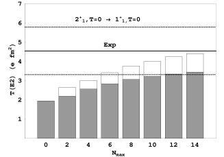
Here we analyze the nature of the transitions in 6Li. There are only one-body and two-body contributions to total matrix elements in the case of two valence particles in the p-shell. Thus, we may determine exactly the one-body and two-body (without using secondary charges) contents of the matrix elements. In Fig. 4 we show the one- and two-body contributions to the matrix element of the isoscalar transition as a function of .
When the model space becomes large, the two-body contribution to this matrix element becomes a significant contribution. This indicates that isoscalar transitions are renormalized strongly and that higher body correlations are essential in accurately calculating the operator. This is not the goal of this paper to describe the experimental data, but for this particular transition, we are able to reproduce the experimental result, within experimental error, provided that the model space is large enough. It is also interesting to estimate a converged value of this and other E2 matrix elements using an exponential plus constant fit as, we did above for the effective charges. We compare the results of the fit and available experimental data in Table 3.
| , (efm2) | |||||
| Eq.(18) | Exp. | ||||
| 12 | 14 | ||||
| 4.25 | 4.42 | 5.59 | 4.5(1.3) | ||
| 4.96 | 5.16 | 6.80 | 8.6(3) | ||
The results presented in Table III indicate that the extrapolated theory gives a reasonable estimate of the available experimental data, taking into account that theoretical NNN forces have not been included in this study.
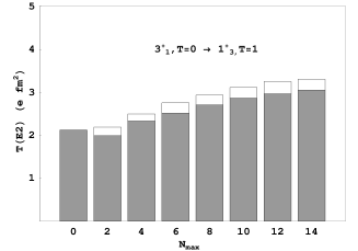
In Fig. 5 we show the one- and two-body contributions to the matrix element of the isovector transition as a function of . Note that in this case the two-body contribution is relatively small and that the total matrix element renormalizes very weakly as the model space increases. Therefore, we can see an indication that isovector transitions are not strongly-dependent on higher-body correlations. Such behavior for the isovector transitions has been noted before by the authors in Nav97 .
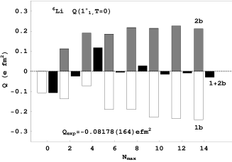
III.3 Role of two-body components for the quadrupole moment of 6Li
The quadrupole moment of 6Li is notoriously difficult to calculate in the shell-model approach. We will now present some insight as to why that may be the case. In Fig. 6 we show the one- and two-body components of the quadrupole moment as a function of increasing model space size. One can immediately draw the interesting conclusion that the one- and two-body contributions are similar in size, yet have opposite signs relative to each other. The two contributions, thus, tend to cancel each other to give a small resultant quadrupole moment. The calculation in the space yields a quadrupole moment e fm2. We were also able to calculate the quadrupole moment in the larger, space, where the dimension of the model space exceeds 805 million. The obtained value, efm2, is very close to the one for the space. Note that even in the largest model space (16 ) calculation, our calculated quadrupole moment, e fm2, is about a factor of 2.5 times too small, when compared to the experimentally measured value of efm2 Cederberg98 . However, the NCSM calculation with the CD-Bonn potential for MeV in the space results in efm2. The NCSM results in the same space with the same frequency, MeV, but with the N3LO interaction Nav04 yield a slightly different value, -0.06 efm2. Again, our goal here is not to reproduce experiment, but to understand the physics of how other physical operators, such as the operator, are renormalized due to truncation of the model space. In the above case, we conclude that the small quadrupole moment for 6Li comes from an almost total cancellation between the one- and two-body contributions, arising from the many-body correlations in the five- and six-body clusters, respectively.
III.4 Applications to the standard-shell model
We now turn our attention to testing our effective operator represented in terms of effective charges. In order to do this, we perform a SSM calculation of transitions for 7Li and 9Li and compare the results to the NCSM calculations. In the SSM calculations, we use the effective operator created from a NCSM calculation specific to the two-body valence cluster approximation for each nucleus. We will refer to these effective interactions for 7(9)Li as the A7(9) interaction, respectively.
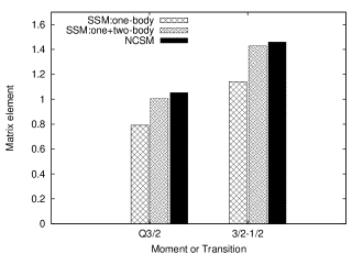
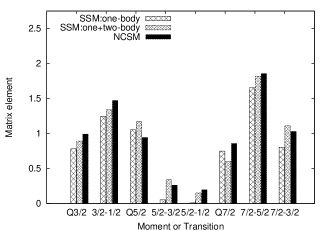
We can see in both figures that using only the one-body effective charges is not sufficient to reproduce the equivalent NCSM matrix element. The secondary effective charges add (in general) a small finite contribution to the SSM matrix element, thereby approximating the NCSM matrix element more accurately. This is particularly evident in 9Li for the and transitions and the quadrupole moment of the state. However, in the case of the quadrupole moment for the and states, for instance, two-body contributions modeled using secondary effective charges do not correctly approximate the two-body parts of the E2 effective operator. This indicates that exact two-body E2 matrix elements have to be used in order to obtain consistent information about interference of one- and two-body contributions. Furthermore, there are higher-body correlations, which have been neglected (e.g. the 3-body effective interaction and the 3-body effective E2 matrix elements).
IV Conclusion
We have constructed effective E2 operators for p-shell, which account exactly for up-to 6-body correlations in the space. Our results indicate that 3- and higher-body correlations strongly renormalize the E2 operators, enhancing the proton part by about 70 and the neutron part by about 40 relative to the bare proton part of the E2 operator. Using 1-body valence cluster (1BVC) and 2-body valence cluster (2BVC) approximations, we have decomposed the effective E2 operator into one-body and two-body parts, where the effective one-body part accounts for up-to 5-body correlations in the space and the effective two-body for residual 6-body correlations in the space. We have found that the proton two-body part of the effective E2 operator constitutes on average about 17 of the total proton renormalization, while the neutron two-body renormalization is about 50 of the total neutron enhancement. Furthermore, we noted that the renormalization for the one-body nondiagonal matrix element, , is about 20 stronger than for the diagonal one, . We have shown that the two-body part of the effective E2 operator can be accounted for reasonably well by introducing secondary effective quadrupole charges. This approximation can be used when the E2 matrix elements are on the scale of 1.0 efm2. However, for small matrix elements (0.2 efm2) the effective two-body part has to be calculated exactly to reproduce the considerable two-body effects. The best illustration of this effect is the case of the 6Li ground state, when one-body and two-body contributions interfere destructively, resulting in a nearly vanishing quadrupole moment.
We have also shown that our effective E2 operators can be used to approximately calculate the quadrupole moment and E2 transitions for heavier nuclei in the SSM formalism (see for, e.g., Fig.(7) and Fig.(8)). Such calculations are useful in predicting what a NCSM calculation for the E2 operator would yield, provided it could be carried out on a sufficiently large computer. Recall that near the center of a major shell, such as the p-shell, the number of basis states involved in performing a converged NCSM calculation would be computationally expensive. However, as we have shown, a SSM calculation is easily performed and gives a good estimate of what the NCSM result for the E2 operator would be.
V Acknowledgments
We thank the Department of Energy’s Institute for Nuclear Theory at the University of Washington for its hospitality and the Department of Energy for partial support during the completion of this work. B.R.B. and A.F.L. acknowledge partial support of this work from NSF grants PHY0244389 and PHY0555396; P.N. acknowledges support in part by the U.S. DOE/SC/NP (Work Proposal N. SCW0498) and U.S Department of Energy Grant DE-FC02-07ER41457; Prepared by LLNL under Contract No. DE-AC52-07NA27344. J.P.V. acknowledges support from U.S. Department of Energy Grants DE-FG02-87ER40371, DE-FC02-07ER41457, and DE-FC02-09ER41582; B.R.B. thanks the GSI Helmholzzentrum für Schwerionenforschung Darmstadt, Germany, for its hospitality during the preparation of this manuscript and the Alexander von Humboldt Stiftung for its support.
References
- (1) P. Navratil, J.P.Vary, B.R.Barrett, Phys. Rev. Lett. 84, 5728 (2000); Phys. Rev. C. 62, 054311 (2000).
- (2) P. Navratil and W.E.Ormand, Phys. Rev. Lett. 88, 152502 (2002); Phys. Rev. C. 68, 034305 (2003).
- (3) I. Stetcu, B.R.Barrett, P.Navratil, J.P.Vary, Phys. Rev. C. 71, 044325 (2005).
- (4) A. Nogga, P.Navratil, B.R.Barrett, J.P.Vary, Phys. Rev. C. 73, 064002 (2006).
- (5) P. Navratil, V. G. Gueorgiev, J.P. Vary, W. E. Ormand, and A. Nogga, Phys. Rev. Lett. 99, 042501 (2007).
- (6) S. C. Pieper, K. Varga, and R. B. Wiringa, Phys. Rev. C 66, 044310 (2002).
- (7) S. Pieper and R. B. Wiringa, Annu. Rev. Nucl. Part. Sci. 51, 53 (2001).
- (8) K.Kowalski, D.J.Dean, M.Hjorth-Jensen, T.Papenbrock, P.Piecuch, Phys. Rev. Lett. 92, 132501 (2004).
- (9) R. Roth and P. Navratil, Phys. Rev. Lett. 99, 092501 (2007).
- (10) A. F. Lisetskiy, B. R. Barrett, M. K. G. Kruse, P.Navratil, I. Stetcu, J. P. Vary, Phys. Rev. C. 78, 044302 (2008).
- (11) R. Machleidt, Phys. Rev. C. 63, 024001 (2001).
- (12) E. Caurier and F. Nowacki, Acta. Phys. Pol. B30, (1999) 705.
- (13) E. Caurier, G. Martinez-Pinedo, F. Nowacki, A. Poves, J. Retamosa, and A. P. Zuker, Phys. Rev. C 59, 2033 (1999).
- (14) E. Caurier, P. Navratil, W. E. Ormand, and J.P. Vary, Phys. Rev. C 64, 051301(R) (2001).
- (15) P. J. Brussaard and P.W.M. Glaudemans, Shell model applications in nuclear spectroscopy, North-Holland Publishing Company, (1977); p.417.
- (16) C. Forssén, J. P. Vary, E. Caurier, and P. Navratil, Phys. Rev. C 77, 024301 (2008).
- (17) P. Navratil, M. Thoresen, and B. R. Barrett, Phys. Rev. C. 55, R573 (1997).
- (18) J. Cederberg et al, Phys. Rev. A. 57, 2539 (1998).
- (19) P. Navratil and E. Caurier, Phys. Rev. C 69, 014311 (2004).