Equalization for Non-Coherent UWB Systems with Approximate Semi-Definite Programming

Abstract

In this paper, we propose an approximate semi-definite programming framework for demodulation and equalization of non-coherent ultra-wide-band communication systems with inter-symbol-interference. It is assumed that the communication systems follow non-linear second-order Volterra models. We formulate the demodulation and equalization problems as semi-definite programming problems. We propose an approximate algorithm for solving the formulated semi-definite programming problems. Compared with the existing non-linear equalization approaches, such as in [1], the proposed semi-definite programming formulation and approximate solving algorithm have low computational complexity and storage requirements. We show that the proposed algorithm has satisfactory error probability performance by simulation results. The proposed non-linear equalization approach can be adopted for a wide spectrum of non-coherent ultra-wide-band systems, due to the fact that most non-coherent ultra-wide-band systems with inter-symbol-interference follow non-linear second-order Volterra signal models.

I Introduction

Ultra-Wide-Band (UWB) communication systems have attracted much attention recently. The UWB communication systems have many advantages including multi-path diversity, low possibilities of intercept and high location estimation accuracy. However, UWB systems also present many challenges compared with narrow-band communication systems. Especially, the communication channels are frequency selective with a large number of resolvable multi-paths. Accurate estimation of channel impulse responses is complex and difficult.

Existing modulation schemes for UWB can be roughly classified into two categories, coherent modulation schemes and non-coherent modulation schemes. The coherent schemes include direct-sequence UWB and multi-band UWB [2] [3] [4]. In these schemes, the demodulation usually depends on accurate estimation of channel impulse responses. The coherent schemes can achieve higher transmission rates. However, their complexity and cost are usually high.

Unlike the coherent modulation schemes, in the non-coherent UWB modulation schemes, the demodulation usually does not depend on full knowledge of channel impulse responses. Therefore, the difficulty of channel estimation is largely avoided. The non-coherent schemes include various differential encoding schemes, and energy detection based schemes (see for example [5] [6] [7]).

One difficulty with the non-coherent modulation schemes is that the signal models are non-linear, if there exists Inter-Symbol-Interference (ISI) in the systems [8] [7]. The existing linear equalization approaches generally do not work well for such non-linear ISI. Because the UWB channels usually have long delay spreads, the approach that increases the spaces between symbols to avoid ISI, severally limits the achievable rates, and therefore is not realistic.

In [1], a new non-linear equalization scheme based on Semi-Definite Programming (SDP) has been proposed. It is shown that even though the SDP relaxation approach is sub-optimal, the performance loss is usually negligible. In [1], an off-the-shelf general-purpose algorithm is adopted to solve the SDP programming problems.

However, general-purpose SDP solving algorithms may not be suitable choices for the UWB demodulation and equalization scenarios. First, the general-purpose algorithms are usually designed to obtain very accurate optimization solutions. While, in the UWB demodulation and equalization scenarios, only approximate solutions are needed to ensure low demodulation errors, because the SDP optimization solutions are only intermediate results. By relaxing the requirement on the accuracy of optimization solutions, the computational complexity can be greatly reduced. Second, the general-purpose SDP solving algorithms do not utilize problem structures. In fact, the computational complexity can be largely reduced by utilizing the structure of the problems.

In this paper, we propose a new iterative algorithm for solving the SDP programming problems. The proposed algorithm has low computational complexity and storage requirements, which make it an attractive choice for low-complexity high-speed implementations. First, the algorithm can achieve a close approximate solution of the optimization problem after only a few iterations. Second, during each iteration, only one optimization problem with much smaller problem size needs to be solved. More precisely, the problem size is equal to the number of bits in one signal block, while, the problem size of the original matrix optimization is proportional to the square of the number of bits in one signal block. The correctness and convergence of the algorithm is proven in this paper. We also show by simulation results that the demodulation and equalization algorithm has satisfactory error probability performance.

In this paper, we demonstrate the performance of the proposed non-linear demodulation and equalization scheme on differential UWB systems. In fact, the proposed algorithm can also be applied on other non-coherent UWB systems, because many non-coherent UWB systems have the same non-linear second-order Volterra signal models. One thing we wish to stress is that certain channel parameter estimation is needed in the proposed demodulation algorithm. However, the estimated model is at the symbol level, rather than at the Nyquist frequency level. The complexity of this partial channel estimation is acceptable.

The rest of this paper is organized as follows. In Section II, we describe the signal model. The SDP problem formulation is presented in Section III. We present the proposed demodulation and equalization algorithm in Section IV. Numerical results are presented in Section V. Conclusions are presented in Section VI.

Notation: we use the symbol $\boldsymbol{\mathcal{S}}$ to denote the set of symmetric matrices. Matrices are denoted by upper bold face letters and column vectors are denoted by lower bold face letters. We use $\boldsymbol{A}\succeq 0$ to denote that the matrix $\boldsymbol{A}$ is positive semi-definite. We use $\boldsymbol{a}\geq 0$ to denote that the elements of the vector $\boldsymbol{a}$ are non-negative. We use $\boldsymbol{A}_{i,j}$ to denote the element of the matrix $\boldsymbol{A}$ at the $i$-th row and $j$-th column. We use $\boldsymbol{a}_{i}$ to denote the $i$-th element of the vector $\boldsymbol{a}$. We use $\boldsymbol{A}^{t}$ and $\boldsymbol{a}^{t}$ to denote the transpose of the matrix $\boldsymbol{A}$ and the vector $\boldsymbol{a}$ respectively. We use $tr(\boldsymbol{A})$ to denote the trace of the matrix $\boldsymbol{A}$. We use $\boldsymbol{A}\cdot\boldsymbol{B}$ to denote the inner product of matrices $\boldsymbol{A}$ and $\boldsymbol{B}$, that is $\boldsymbol{A}\cdot\boldsymbol{B}=tr(\boldsymbol{A}^{t}\boldsymbol{B})$. The function $\mbox{sign}(\cdot)$ is defined as,

$$\mbox{sign}(x)=\left\{\begin{array}[]{ll}1,&\mbox{if }x\geq 0,\\ -1,&\mbox{otherwise}.\end{array}\right.$$ (3)

II Signal Model

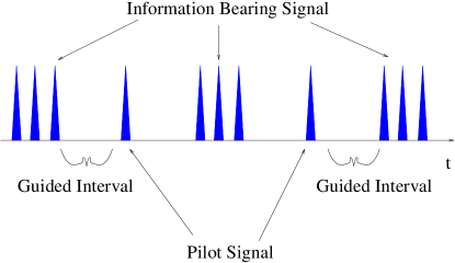
Figure 1: signal is transmitted in a block by block fashion

In this paper, we consider the differential UWB systems. We assume that information is transmitted in a block by block fashion as shown in Fig. 1. That is, the transmitted signal $s(t)$ can be written as,

$$s(t)=\sum_{k=0}^{\infty}s_{k}^{i}(t-kT_{b})+\sum_{k=0}^{\infty}s_{k}^{p}(t-kT_{b}-\tau_{k})$$ (4)

where $s_{k}^{i}(t)$ is the signal waveform for the $k$th block of information bearing signals, and $s_{k}^{p}(t)$ is the waveform for the $k$th block of pilot signals.

The waveform for one block of information bearing signals can be written as,

$$s_{k}^{i}(t)=\sum_{n=0}^{N_{b}-1}\sum_{i=0}^{N_{p}-1}a_{i}[n]\bar{w}\left(t-t_{i}[n]\right)$$ (5)

where $\bar{w}(t)$ is the transmitted pulse, $a_{i}[n]$ is the pulse polarity for the $i$-th pulse of the $n$-th symbol, $t_{i}[n]$ is the pulse time for the $i$-th pulse of the $n$-th symbol. Each block has $N_{b}$ symbols, and each symbol corresponds to $N_{p}$ pulses.

Denote the data symbol by $d[n]\in\{-1,+1\}$. The data symbols are differentially encoded as,

$$a_{i}[n]=\left\{\begin{array}[]{ll}a_{N_{p}-1}[n-1]d[n-1]b_{N_{p}-1},&\mbox{ if }i=0\\ a_{i-1}[n]d[n]b_{i-1},&\mbox{ otherwise}\end{array}\right.$$ (8)

where, $b_{0},b_{1},\ldots,b_{N_{p}-1}$ is the pseudo-random amplitude code sequence, $b_{i}\in\{-1,+1\}$. The pulse time

$$t_{i}[n]=nT_{s}+c_{i}$$ (9)

where $T_{s}$ is the symbol duration, $c_{i}$ is the relative pulse timing.

The pilot signal $s_{k}^{p}(t)$ is introduced to facilitate timing synchronization and partial channel estimation. Guided intervals are introduced between blocks of information bearing signals and pilot signals, so that all inter-block-interference is avoided.

Similarly as in [1], at the receiver side, an auto-correlation receiver is used. Denote the received signals corresponding to one block of information bearing signals by $z[m]$, $m=1,2,\ldots,N_{r}$. The signal model of the system is a second-order Volterra model as follows.

$$z[m]=(\boldsymbol{r}+\boldsymbol{P}\boldsymbol{d})^{t}\boldsymbol{Q}^{t}\boldsymbol{B}[m]\boldsymbol{Q}(\boldsymbol{r}+\boldsymbol{P}\boldsymbol{d})+\mbox{ noise terms,}$$ (10)

where $\boldsymbol{Q}$, $\boldsymbol{P}$, $\boldsymbol{r}$ are constant matrices and vectors , and $\boldsymbol{B}[n]$ are matrices that depends on the wireless channel (more detailed definitions can be found in [1]). We assume that the matrices $\boldsymbol{B}[m]$ can be estimated accurately by using the pilot signals.

III SDP Problem Formulation

Similarly as in [1], we reformulate the difficult discrete optimization problem into a matrix optimization and relax it into an SDP problem. The SDP formulation in this paper is slightly different from the one in [1]. Instead of introducing auxiliary variables, we formulate the SDP problem with the following convex objective function f(U).

$$f(\boldsymbol{U})=\sum_{m=1}^{N_{r}}\left\{z[m]-\boldsymbol{r}^{t}\boldsymbol{Q}^{t}\boldsymbol{B}[m]\boldsymbol{Q}\boldsymbol{r}-\boldsymbol{r}^{t}\boldsymbol{Q}^{t}\boldsymbol{B}[m]\boldsymbol{Q}\boldsymbol{P}\boldsymbol{d}\right.$$

$$-\left.\boldsymbol{r}^{t}\boldsymbol{Q}^{T}\boldsymbol{B}[m]^{t}\boldsymbol{Q}\boldsymbol{P}\boldsymbol{d}-tr\left\{\boldsymbol{D}\boldsymbol{P}^{t}\boldsymbol{Q}^{t}\boldsymbol{B}[m]\boldsymbol{Q}\boldsymbol{P}\right\}\right\}^{2},$$ (11)

where $\boldsymbol{U}$ is a $N_{b}+1$ by $N_{b}+1$ positive semi-definite symmetric matrix, $\boldsymbol{D}$ denote the sub-matrix of $\boldsymbol{U}$ formed by selecting the last $N_{b}$ rows and columns, and $\boldsymbol{d}$ is a vector $\boldsymbol{d}=[\boldsymbol{U}_{1,2},\ldots,\boldsymbol{U}_{1,N_{b}+1}]^{t}$

The convex SDP problem is summarized as follows.

$$\min f(\boldsymbol{U})$$

subject to: $$\boldsymbol{U}_{n,n}=1,\mbox{ for all }n,$$ (12)

$$\boldsymbol{U}\in\boldsymbol{\mathcal{S}},$$ (13)

$$\boldsymbol{U}\succeq 0.$$ (14)

The demodulation result is obtained from the solution of the above SDP problem by thresholding. That is, the demodulation result for the $n$th symbol is obtained as $\mbox{sign}(\boldsymbol{U}_{1,n+1})$.

IV Approximate Semi-definite Programming Algorithm

In this section, we propose a new approximate algorithm of solving semi-definite programming. The algorithm is a generalization of Hazan’s algorithm on approximate semi-definite programming [9]. Hazan’s algorithm considers a special class of SDP optimization problems, where the constraints are total trace constraints. Such SDP optimization problems usually arise in Quantum State Tomograph (QST) problems. The algorithm proposed in this paper considers the class of problems with the constraints that the diagonal elements of the matrix must be one.

We consider the following SDP optimization problem.

$$\min f(\boldsymbol{X})$$

subject to: $$\mbox{ diagonal elements of }\boldsymbol{X}\mbox{ are zeros},$$

$$\boldsymbol{X}\mbox{ is symmetric},$$

$$\boldsymbol{X}+\boldsymbol{I}\succeq 0,$$ (15)

where, $\boldsymbol{X}$ is a square matrix, $\boldsymbol{I}$ is the identity matrix with the same numbers of rows and columns. Without loss of generality, we assume that $f(\cdot)$ is independent of the diagonal elements of the matrix $\boldsymbol{X}$. We also assume that $f(\cdot)$ has a bounded curvature constant $C_{f}$. The curvature constant $C_{f}$ is defined as follows.

$$C_{f}=\sup\frac{1}{\beta^{2}}\left[f(\boldsymbol{Y})-f(\boldsymbol{X})+(\boldsymbol{Y}-\boldsymbol{X})^{t}\bigtriangledown f(\boldsymbol{X})\right]$$ (16)

where, $\boldsymbol{X}+\boldsymbol{I}\succeq 0,\boldsymbol{Z}+\boldsymbol{I}\succeq 0,\boldsymbol{Y}=\boldsymbol{X}+\beta(\boldsymbol{Z}-\boldsymbol{X})$, and all diagonal elements of $\boldsymbol{X}$, $\boldsymbol{Y}$, $\boldsymbol{Z}$ are zeros. Clearly, the convex-SDP optimization problem in the previous section can be reduced into the above optimization problem and solved.

Before going into details of the proposed algorithm, we need some basic facts on matrices. These facts will be presented in Section IV-A. The dual function of $f(\boldsymbol{X})$ will be discussed in Section IV-B. The algorithm will be presented in Section IV-C. The correctness and convergence of the algorithm will be proved in Section IV-D. Certain discussions will be presented in Section IV-E.

IV-A Some Basic Facts

Lemma IV.1

Let $\boldsymbol{X}$ be a symmetric matrix with all the diagonal elements being zero. Then $\boldsymbol{I}+\boldsymbol{X}$ is positive semi-definite, if and only if $\lambda_{\min}(\boldsymbol{X})\geq-1$, where $\lambda_{\min}(\boldsymbol{X})$ denotes the smallest eigenvalue of $\boldsymbol{X}$.

Proof:

Necessary condition: assume that $\boldsymbol{X}$ is positive semi-definite, then

$$\lambda_{\min}(\boldsymbol{X}) =\min_{||\boldsymbol{v}||=1}\boldsymbol{v}^{t}\boldsymbol{X}\boldsymbol{v},$$

$$=\min_{||\boldsymbol{v}||=1}\boldsymbol{v}^{t}(\boldsymbol{I}+\boldsymbol{X})\boldsymbol{v}-\boldsymbol{v}^{t}\boldsymbol{I}\boldsymbol{v},$$

$$\geq\min_{||\boldsymbol{v}||=1}0-\boldsymbol{v}^{t}\boldsymbol{I}\boldsymbol{v}=-1.$$ (17)

Sufficient condition: It is sufficient to show that $\boldsymbol{v}^{t}(\boldsymbol{I}+\boldsymbol{X})\boldsymbol{v}\geq 0$ for all $\boldsymbol{v}$ with $||\boldsymbol{v}||=1$. The above statement follows from the fact that $\boldsymbol{v}^{t}\boldsymbol{X}\boldsymbol{v}\geq\lambda_{\min}(\boldsymbol{X})||\boldsymbol{v}||^{2}\geq-1$. ∎

Lemma IV.2

Let $\boldsymbol{X}_{1}$ $\boldsymbol{X}_{2}$ be two symmetric matrices, such that the smallest eigenvalues of the matrices are greater than $-1$,

$$\lambda_{\min}(\boldsymbol{X}_{1})\geq-1,\,\,\,\lambda_{\min}(\boldsymbol{X}_{2})\geq-1.$$ (18)

Let $\boldsymbol{X}$ be a linear combination of $\boldsymbol{X}_{1}$ and $\boldsymbol{X}_{2}$. That is $\boldsymbol{X}=\beta\boldsymbol{X}_{1}+(1-\beta)\boldsymbol{X}_{2}$, where $0\leq\beta\leq 1$. Then, the smallest eigenvalue of $\boldsymbol{X}$ is also greater than $-1$,

$$\lambda_{\min}(\boldsymbol{X})\geq-1.$$ (19)

Proof:

$$\lambda_{\min}(\boldsymbol{X}) =\min_{||\boldsymbol{v}||=1}\boldsymbol{v}^{t}\boldsymbol{X}\boldsymbol{v}$$

$$=\min_{||\boldsymbol{v}||=1}\boldsymbol{v}^{t}(\beta\boldsymbol{X}_{1}+(1-\beta)\boldsymbol{X}_{2})\boldsymbol{v}$$

$$\geq\beta(-1)+(1-\beta)(-1)=-1.$$ (20)

∎

IV-B Weak Duality

The proposed algorithm is based on iteratively reducing the duality gap between the primal function and its dual function. For a primal function $f(\boldsymbol{X})$, we define the dual function $w(\boldsymbol{X})$ as

$$w(\boldsymbol{X}) =\max_{\bigtriangledown f(\boldsymbol{X})+\boldsymbol{\lambda}\succeq 0}w(\boldsymbol{X},\boldsymbol{\lambda})$$

$$=\max_{\bigtriangledown f(\boldsymbol{X})+\boldsymbol{\lambda}\succeq 0}f(\boldsymbol{X})-\boldsymbol{X}\cdot\bigtriangledown f(\boldsymbol{X})-tr(\boldsymbol{\lambda}),$$ (21)

where, $\boldsymbol{\lambda}=\mbox{diag}(\lambda_{1},\lambda_{2},\ldots,\lambda_{n})$ is a diagonal matrix.

Theorem IV.3

(Weak Duality) Denote the minimizer of the optimization problem in Eq. IV as $\boldsymbol{X}^{\ast}$. Let $\boldsymbol{X}$ be a feasible point. Then, the following weak duality inequalities hold.

$$f(\boldsymbol{X})\geq f(\boldsymbol{X}^{\ast})\geq w(\boldsymbol{X})$$ (22)

Proof:

Given a function $f(\boldsymbol{X})$, the corresponding Lagrangian function can be written as

$$f(\boldsymbol{X})-\boldsymbol{V}\cdot(\boldsymbol{I}+\boldsymbol{X})+\boldsymbol{\lambda}\cdot\boldsymbol{X}$$ (23)

where $\boldsymbol{V}$ is a symmetric positive semi-definite matrix.

We can rewrite the function $f(\boldsymbol{X}^{\ast})$ in a min-max form as follows.

$$f(\boldsymbol{X}^{\ast})=\min_{\boldsymbol{X}\succeq 0,\boldsymbol{X}\in\mathcal{S}}f(\boldsymbol{X})$$

$$=\min_{\boldsymbol{X}\in\mathcal{S}}\left[\max_{\boldsymbol{V}\succeq 0,\boldsymbol{\lambda}}\left[f(\boldsymbol{X})-\boldsymbol{V}\cdot(\boldsymbol{I}+\boldsymbol{X})+\boldsymbol{\lambda}\cdot\boldsymbol{X}\right]\right]$$ (24)

This is because

$$\max_{\boldsymbol{V}\succeq 0,\boldsymbol{\lambda}}\left[f(\boldsymbol{X})-\boldsymbol{V}\cdot(\boldsymbol{I}+\boldsymbol{X})+\boldsymbol{\lambda}\cdot\boldsymbol{X}\right]$$

$$=\left\{\begin{array}[]{ll}f(\boldsymbol{X}),&\mbox{ if }\boldsymbol{X}\succeq 0\mbox{ and}\\ &\mbox{ diagonal elements of }\boldsymbol{X}\mbox{ are zeros}\\ +\infty,&\mbox{ otherwise }\end{array}\right.$$ (28)

By the max-min inequality (see for example, [10] page 238, Eq. 5.47), we can lower bound $f(\boldsymbol{X}^{\ast})$ as follows.

$$f(\boldsymbol{X}^{\ast})=\min_{\boldsymbol{X}\in\mathcal{S}}\left[\max_{\boldsymbol{V}\succeq 0,\boldsymbol{\lambda}}\left[f(\boldsymbol{X})-\boldsymbol{V}\cdot(\boldsymbol{I}+\boldsymbol{X})+\boldsymbol{\lambda}\cdot\boldsymbol{X}\right]\right]$$

$$\geq\max_{\boldsymbol{V}\succeq 0,\boldsymbol{\lambda}}\left[\min_{\boldsymbol{X}\in\mathcal{S}}\left[f(\boldsymbol{X})-\boldsymbol{V}\cdot(\boldsymbol{I}+\boldsymbol{X})+\boldsymbol{\lambda}\cdot\boldsymbol{X}\right]\right]$$ (29)

Let us assume that $\boldsymbol{V}_{0}$ and $\boldsymbol{\lambda}_{0}$ are symmetric and diagonal matrix respectively, such that the following equations hold for a feasible point $\boldsymbol{X}_{0}$.

$$\bigtriangledown f(\boldsymbol{X}_{0})-\boldsymbol{V}_{0}+\boldsymbol{\lambda}_{0}=\boldsymbol{0},$$ (30)

$$\bigtriangledown f(\boldsymbol{X}_{0})+\boldsymbol{\lambda}_{0}\succeq 0.$$ (31)

By the above discussions, we have

$$f(\boldsymbol{X}^{\ast})$$

$$\geq\max_{\boldsymbol{V}\succeq 0,\boldsymbol{\lambda}}\left[\min_{\boldsymbol{X}\in\mathcal{S}}\left[f(\boldsymbol{X})-\boldsymbol{V}\cdot(\boldsymbol{I}+\boldsymbol{X})+\boldsymbol{\lambda}\cdot\boldsymbol{X}\right]\right],$$

$$\geq\min_{\boldsymbol{X}\in\mathcal{S}}\left[f(\boldsymbol{X})-\boldsymbol{V}_{0}\cdot(\boldsymbol{I}+\boldsymbol{X})+\boldsymbol{\lambda}_{0}\cdot\boldsymbol{X}\right],$$

$$\stackrel{{\scriptstyle(a)}}{{=}}f(\boldsymbol{X}_{0})-\boldsymbol{V}_{0}\cdot(\boldsymbol{I}+\boldsymbol{X}_{0})+\boldsymbol{\lambda}_{0}\cdot\boldsymbol{X}_{0},$$

$$\stackrel{{\scriptstyle(b)}}{{=}}f(\boldsymbol{X}_{0})-(\bigtriangledown f(\boldsymbol{X}_{0})+\boldsymbol{\lambda}_{0})\cdot(\boldsymbol{I}+\boldsymbol{X}_{0})+\boldsymbol{\lambda}_{0}\cdot\boldsymbol{X}_{0},$$

$$=f(\boldsymbol{X}_{0})-\bigtriangledown f(\boldsymbol{X}_{0})\cdot\boldsymbol{X}-\boldsymbol{\lambda}_{0}\cdot\boldsymbol{I},$$ (32)

where, (a) follows from the fact that $\boldsymbol{X}_{0}$ is exactly the minimizer, and (b) follows from the definition of $\boldsymbol{V}_{0}$. Therefore,

$$f(\boldsymbol{X}^{\ast}) \geq\max_{\bigtriangledown f(\boldsymbol{X}_{0})+\boldsymbol{\lambda}\succeq 0}f(\boldsymbol{X}_{0})-\boldsymbol{X}_{0}\cdot\bigtriangledown f(\boldsymbol{X}_{0})-tr(\boldsymbol{\lambda}),$$

$$\geq w(\boldsymbol{X}_{0}).$$ (33)

The theorem follows from the fact that $\boldsymbol{X}_{0}$, $\boldsymbol{V}_{0}$, and $\boldsymbol{\lambda}_{0}$ are arbitrary. ∎

The above weak duality theorem provides a way to estimate how far a feasible point $\boldsymbol{X}$ is away from the optimal solution. We define

$$h(\boldsymbol{X})=f(\boldsymbol{X})-f(\boldsymbol{X}^{\ast}),$$ (34)

$$g(\boldsymbol{X})=f(\boldsymbol{X})-w(\boldsymbol{X}).$$ (35)

By the weak duality theorem, we have $h(\boldsymbol{X})\leq g(\boldsymbol{X})$.

In order to evaluate the dual function $w(\boldsymbol{X})$, the following optimization problem needs to be solved.

$$\min\sum_{i}\lambda_{i}$$

$$\mbox{subject to }\gamma_{i}\geq 0,\mbox{ for all }i$$ (36)

where $\gamma_{i}$ is the $i$th eigenvalue of the matrix $\bigtriangledown f(\boldsymbol{X})+\boldsymbol{\lambda}$.

Lemma IV.4

Let $\gamma_{i}$ denote the $i$th eigenvalue of the matrix $\bigtriangledown f(\boldsymbol{X})+\boldsymbol{\lambda}$. Let $\boldsymbol{v}_{i}$ denote the corresponding eigenvectors. Then,

$$\Delta\gamma_{i}=\sum_{j}(v_{ij})^{2}\Delta\lambda_{i}$$ (37)

where, $\Delta\gamma_{i}$ and $\Delta\lambda_{i}$ are the infinitesimal differences, $v_{ij}$ denotes the $j$th element of the vector $\boldsymbol{v}_{i}$.

Proof:

It is clear that there exists a decomposition of $\bigtriangledown f(\boldsymbol{X})+\boldsymbol{\lambda}$,

$$\bigtriangledown f(\boldsymbol{X})+\boldsymbol{\lambda}=\boldsymbol{V}\boldsymbol{\Lambda}\boldsymbol{V}^{t}$$ (38)

such that $\boldsymbol{V}$ is a unitary matrix and $\Lambda$ is a diagonal matrix. In fact, $\boldsymbol{V}=[\boldsymbol{v}_{1},\boldsymbol{v}_{2},\ldots,\boldsymbol{v}_{n}]$ and $\Lambda=\mbox{diag}(\gamma_{i})$ is a such decomposition.

Let $\Delta\boldsymbol{V}$ and $\Delta\boldsymbol{\Lambda}$ be the corresponding infinitesimal differences of $\boldsymbol{V}$ and $\boldsymbol{\Lambda}$ respectively. Then, we have

$$(\boldsymbol{V}+\Delta\boldsymbol{V})(\boldsymbol{\Lambda}+\Delta\boldsymbol{\Lambda})(\boldsymbol{V}^{t}+\Delta\boldsymbol{V}^{t})=\triangledown f(\boldsymbol{X})+\boldsymbol{\lambda}+\Delta\boldsymbol{\lambda},$$ (39)

$$(\boldsymbol{V}^{t}+\Delta\boldsymbol{V}^{t})(\boldsymbol{V}+\Delta\boldsymbol{V})=\boldsymbol{I}.$$ (40)

From Eq. 40 and the fact that $\boldsymbol{V}$ is unitary, we have

$$\boldsymbol{V}^{t}\Delta\boldsymbol{V}+\Delta\boldsymbol{V}^{t}\boldsymbol{V}=0.$$ (41)

Since $\boldsymbol{V}^{t}\Delta\boldsymbol{V}$ and $\Delta\boldsymbol{V}^{t}\boldsymbol{V}$ are the transpose of each other, we conclude that the matrices $\boldsymbol{V}^{t}\Delta\boldsymbol{V}$ and $\Delta\boldsymbol{V}^{t}\boldsymbol{V}$ are anti-symmetric and their diagonal elements are all zeros.

From Eq. 39, we have

$$\boldsymbol{V}\Delta\boldsymbol{\Lambda}\boldsymbol{V}^{t}+\Delta\boldsymbol{V}\boldsymbol{\Lambda}\boldsymbol{V}^{t}+\boldsymbol{V}\boldsymbol{\Lambda}\Delta\boldsymbol{V}^{t}=\Delta\boldsymbol{\lambda}.$$ (42)

Multiplying the above equation by the matrix $\boldsymbol{V}^{t}$ at the left side and the matrix $\boldsymbol{V}$ at the right side, we obtain

$$\Delta\boldsymbol{\Lambda}+\boldsymbol{V}^{t}\Delta\boldsymbol{V}\boldsymbol{\Lambda}+\boldsymbol{\Lambda}\Delta\boldsymbol{V}^{t}\boldsymbol{V}=\boldsymbol{V}^{t}\Delta\boldsymbol{\lambda}\boldsymbol{V}.$$ (43)

Since the diagonal elements of the matrices $\boldsymbol{V}^{t}\Delta\boldsymbol{V}$ and $\Delta\boldsymbol{V}^{t}\boldsymbol{V}$ are all zeros, the diagonal elements of the matrices $\boldsymbol{V}^{t}\Delta\boldsymbol{V}\boldsymbol{\Lambda}$ and $\boldsymbol{\Lambda}\Delta\boldsymbol{V}^{t}\boldsymbol{V}$ are also zeros. Therefore, we conclude that the diagonal elements of $\Delta\boldsymbol{\Lambda}$ and $\boldsymbol{V}^{t}\Delta\boldsymbol{\lambda}\boldsymbol{V}$ are identical. The theorem then follows from the fact that the $i$th diagonal element of the matrix $\boldsymbol{V}^{t}\Delta\boldsymbol{\lambda}\boldsymbol{V}$ is $\sum_{j}({v}_{ij})^{2}\Delta\lambda_{j}$. ∎

Lemma IV.5

In the optimization problem in Eq. IV-B. Let $\boldsymbol{\lambda}^{\ast}$ be the minimizer. Let $\gamma_{i}$ denote the $i$th eigenvalue of the matrix $\bigtriangledown f(\boldsymbol{X})+\boldsymbol{\lambda}^{\ast}$. Let $\boldsymbol{v}_{i}$ denote the corresponding eigenvectors. Then, there exist a set ${\mathcal{T}}\subset\{1,2,\ldots,n\}$ and a vector $\boldsymbol{y}$, such that

$$\boldsymbol{y}\geq 0,$$ (44)

$$\boldsymbol{V}^{t}\boldsymbol{y}=[1,\ldots,1]^{t},$$ (45)

$$\boldsymbol{v}_{i}^{t}\left(\bigtriangledown f(\boldsymbol{X})+\boldsymbol{\lambda}^{\ast}\right)\boldsymbol{v}_{i}=0,\mbox{ for all }i\in{\mathcal{T}},$$ (46)

where $n$ is the number of rows of matrix $\boldsymbol{\lambda}$, $\boldsymbol{V}$ is a matrix such that each row of $\boldsymbol{V}$ is $[v_{ij}^{2}]$ for one $i\in{\mathcal{T}}$. That is,

$$\boldsymbol{V}=\left[\begin{array}[]{cccc}v_{i_{1},1}^{2}&v_{i_{2},2}^{2}&\ldots&v_{i_{1},n}^{2}\\ \ldots&\ldots&\ldots&\ldots\\ v_{i_{k},1}^{2}&v_{i_{k},2}^{2}&\ldots&v_{i_{k},n}^{2}\end{array}\right],$$ (50)

where $i_{1},\ldots,i_{k}\in{\mathcal{T}}$.

Proof:

Due to the nature of the optimization problem, there exist at least one active constraint at the minimizer. We say that an inequality constraint is active at a feasible point, if the inequality constraint holds with equality. In this optimization problem, the $i$th inequality constraint is active, if $\gamma_{i}=0$. Let $\mathcal{T}$ denote the set of indexes of all active constraints. Then, for all $i\in{\mathcal{T}}$, $\gamma_{i}=0$,

$$\boldsymbol{v}_{i}^{t}\left(\bigtriangledown f(\boldsymbol{X})+\boldsymbol{\lambda}^{\ast}\right)\boldsymbol{v}_{i}=0.$$ (51)

Due to the Karush-Kuhn-Tucker (KKT) Theorem ( see [11] Theorem 20.1 . Page 398), there exists a vector $\boldsymbol{y}$ such that

$$\boldsymbol{y}\geq 0,$$ (52)

$$\sum_{i}y_{i}\bigtriangledown\gamma_{i}=\bigtriangledown{\sum_{i}\lambda_{i}}=[1,1,\ldots,1]^{t}.$$ (53)

According to Lemma IV.4, $\bigtriangledown\gamma_{i}=[v_{i1}^{2},v_{i2}^{2},\ldots,v_{in}^{2}]^{t}$. Therefore

$$\sum_{i}y_{i}\bigtriangledown\gamma_{i}=\boldsymbol{V}^{t}\boldsymbol{y}$$ (54)

The lemma follows. ∎

Corollary IV.6

For $i\in{\mathcal{T}}$, define $\alpha_{i}=\boldsymbol{v}_{i}^{t}\bigtriangledown f(\boldsymbol{X})\boldsymbol{v}_{i}$. Then,

$$\sum_{i}\lambda_{i}^{\ast}=-\sum_{i\in{\mathcal{T}}}y_{i}\alpha_{i}$$ (55)

Proof:

$$\sum_{i}\lambda_{i}^{\ast} =[1,\ldots,1]\mbox{diag}(\boldsymbol{\lambda}^{\ast})=\boldsymbol{y}^{t}\boldsymbol{V}(\mbox{diag}(\boldsymbol{\lambda}^{\ast}))$$

$$=\boldsymbol{y}^{t}\left[\ldots,\sum_{j}(v_{ij})^{2}\lambda_{j},\ldots\right]^{t}$$

$$=\boldsymbol{y}^{t}\left[\ldots,\boldsymbol{v_{i}}^{t}\boldsymbol{\lambda}^{\ast}\boldsymbol{v}_{i},\ldots\right]^{t}$$

$$\stackrel{{\scriptstyle(a)}}{{=}}\boldsymbol{y}^{t}\left[\ldots,-\alpha_{i},\ldots\right]^{t}$$

$$=-\sum_{i\in{\mathcal{T}}}y_{i}\alpha_{i},$$ (56)

where, $\mbox{diag}(\boldsymbol{\lambda}^{\ast})$ denote the column vector that consists of diagonal elements of $\boldsymbol{\lambda}^{\ast}$, and (a) follows from Eq. 46. ∎

IV-C The Algorithm

The proposed algorithm is summarized as follows.

• Step 1: set k=1, set $\boldsymbol{X}$ to a feasible point;

• Step 2: calculate the gradient $\bigtriangledown f(\boldsymbol{X})$;

• Step 3: solve the optimization problem in Eq. IV-B, obtain $\alpha_{i}$, $y_{i}$, $\boldsymbol{v}_{i}$ for $i\in{\mathcal{T}}$;

• Step 4: calculate the function $g(\boldsymbol{X})$, if $g(\boldsymbol{X})$ is less than a certain threshold, go to step 8, otherwise, go to the next step;

• Step 5: update $\Delta\boldsymbol{X}$ as follows,

  $$\Delta\boldsymbol{X}=\beta_{k}\left(\left(\sum_{i\in{\mathcal{T}}}y_{i}\boldsymbol{v}_{i}\boldsymbol{v}_{i}^{t}\right)-\boldsymbol{X}-\boldsymbol{I}\right)$$ (57)

  where, $\beta_{k}$ is a predefined step size parameter;

• Step 6: update $\boldsymbol{X}=\boldsymbol{X}+\Delta\boldsymbol{X}$;

• Step 7: set k=k+1, go to step 2;

• Step 8: return $\boldsymbol{X}$, stop.

IV-D Correction and Convergence

In this subsection, we show that the proposed algorithm is correct and converges.

Theorem IV.7

In the proposed algorithm, the diagonal elements of $\boldsymbol{X}$ are zeros, and $\lambda_{\min}(\boldsymbol{X})\geq-1$.

Proof:

Prove by induction. It is sufficient to show that $\boldsymbol{X}+\Delta\boldsymbol{X}$ satisfies the above conditions, if $\boldsymbol{X}$ satisfies the conditions.

Note that the $k$th diagonal element of the matrix $\sum_{i\in{\mathcal{T}}}y_{i}\boldsymbol{v}_{i}\boldsymbol{v}_{i}^{t}$ is equal to $\sum_{i\in{\mathcal{T}}}y_{i}v_{ik}^{2}$, is also equal to the $k$th element of $\boldsymbol{V}^{t}\boldsymbol{y}$. From Lemma IV.5, we have that the $k$th element of $\boldsymbol{V}^{t}\boldsymbol{y}$ is one. Therefore, the diagonal elements of the matrix $\sum_{i\in{\mathcal{T}}}y_{i}\boldsymbol{v}_{i}\boldsymbol{v}_{i}^{t}-\boldsymbol{X}-\boldsymbol{I}$ are all zeros. The diagonal elements of the matrix $\boldsymbol{X}+\Delta\boldsymbol{X}$ are also all zeros.

We can show that $\lambda_{\min}(\boldsymbol{X}+\Delta\boldsymbol{X})\geq-1$, if we can show that

$$\lambda_{\min}\left[\left(\sum_{i\in{\mathcal{T}}}y_{i}\boldsymbol{v}_{i}\boldsymbol{v}_{i}^{t}\right)-\boldsymbol{I}\right]\geq-1,$$ (58)

$$\lambda_{\min}\left(\boldsymbol{X}\right)\geq-1.$$ (59)

This is because of Lemma IV.2 and $\boldsymbol{X}+\Delta\boldsymbol{X}$ being a linear combination of the above two matrices

$$\boldsymbol{X}+\Delta\boldsymbol{X}=\beta_{k}\left(\sum_{i\in{\mathcal{T}}}y_{i}\boldsymbol{v}_{i}\boldsymbol{v}_{i}^{t}-\boldsymbol{I}\right)+(1-\beta_{k})\boldsymbol{X}$$ (60)

Eq. 59 follows from the given hypothesis. Eq. 58 follows from Lemma IV.1, and $\sum_{i\in{\mathcal{T}}}y_{i}\boldsymbol{v}_{i}\boldsymbol{v}_{i}^{t}$ being positive semi-definite. The theorem is proven. ∎

Theorem IV.8

In the proposed optimization algorithm, let $\boldsymbol{X}_{k}$ denote the value of $\boldsymbol{X}$ after $k$ iterations. Then, the gap

$$h(\boldsymbol{X}_{k+1}) \leq(1-\beta_{k})h(\boldsymbol{X}_{k})+\beta_{k}^{2}C_{f}.$$ (61)

Therefore, $h(\boldsymbol{X}_{k})$ goes to zero, and $f(\boldsymbol{X}_{k})$ goes to $f(\boldsymbol{X}^{\ast})$, for properly chosen step size parameters $\beta_{k}$.

Proof:

First, we wish to show that the following equality holds.

$$\left(\sum_{i\in{\mathcal{T}}}y_{i}\boldsymbol{v}_{i}\boldsymbol{v}_{i}^{t}\right)\cdot\bigtriangledown f(\boldsymbol{X})=\sum_{i\in{\mathcal{T}}}y_{i}\alpha_{i}$$ (62)

The reasoning is as follows.

$$\left(\sum_{i\in{\mathcal{T}}}y_{i}\boldsymbol{v}_{i}\boldsymbol{v}_{i}^{t}\right)\cdot\bigtriangledown f(\boldsymbol{X})=\sum_{i\in{\mathcal{T}}}\left(y_{i}\boldsymbol{v}_{i}\boldsymbol{v}_{i}^{t}\cdot\bigtriangledown f(\boldsymbol{X})\right)$$

$$=\sum_{i\in{\mathcal{T}}}\left(tr\left(y_{i}\boldsymbol{v}_{i}\boldsymbol{v}_{i}^{t}\bigtriangledown f(\boldsymbol{X})\right)\right)$$

$$\stackrel{{\scriptstyle(a)}}{{=}}\sum_{i\in{\mathcal{T}}}y_{i}\left(tr\left(\boldsymbol{v}_{i}^{t}\bigtriangledown f(\boldsymbol{X})\boldsymbol{v}_{i}\right)\right)$$

$$=\sum_{i\in{\mathcal{T}}}y_{i}\left(\boldsymbol{v}_{i}^{t}\bigtriangledown f(\boldsymbol{X})\boldsymbol{v}_{i}\right)$$

$$\stackrel{{\scriptstyle(b)}}{{=}}\sum_{i\in{\mathcal{T}}}y_{i}\alpha_{i}$$ (63)

where, (a) follows from the the property of trace, $tr(\boldsymbol{A}\boldsymbol{B})=tr(\boldsymbol{B}\boldsymbol{A})$ for all matrices $\boldsymbol{A}$ and $\boldsymbol{B}$, and (b) follows from the definition of $\alpha_{i}$.

The value of $f(\boldsymbol{X}_{k+1})$ can be upper bounded as follows.

$$f(\boldsymbol{X}_{k+1})=f\left(\boldsymbol{X}_{k}+\beta_{k}\left(\sum_{i\in{\mathcal{T}}}y_{i}\boldsymbol{v}_{i}\boldsymbol{v}_{i}^{t}-\boldsymbol{X}_{k}-\boldsymbol{I}\right)\right)$$

$$\stackrel{{\scriptstyle(a)}}{{\leq}}f(\boldsymbol{X}_{k})+\beta_{k}\left(\sum_{i\in{\mathcal{T}}}y_{i}\boldsymbol{v}_{i}\boldsymbol{v}_{i}^{t}-\boldsymbol{X}_{k}-\boldsymbol{I}\right)\cdot\bigtriangledown f(\boldsymbol{X}_{k})+\beta_{k}^{2}C_{f}$$

$$\stackrel{{\scriptstyle(b)}}{{=}}f(\boldsymbol{X}_{k})+\beta_{k}\left(\left(\sum_{i\in{\mathcal{T}}}y_{i}\boldsymbol{v}_{i}\boldsymbol{v}_{i}^{t}\right)\cdot\bigtriangledown f(\boldsymbol{X}_{k})-\boldsymbol{X}_{k}\cdot\bigtriangledown f(\boldsymbol{X}_{k})\right)$$

$$\hskip 36.135pt+\beta_{k}^{2}C_{f}$$

$$\stackrel{{\scriptstyle(c)}}{{=}}f(\boldsymbol{X}_{k})+\beta_{k}\left(\sum_{i\in{\mathcal{T}}}y_{i}\alpha_{i}-\boldsymbol{X}_{k}\cdot\bigtriangledown f(\boldsymbol{X}_{k})\right)+\beta_{k}^{2}C_{f}$$

$$\stackrel{{\scriptstyle(d)}}{{=}}f(\boldsymbol{X}_{k})+\beta_{k}\left(-\sum_{i}\lambda_{i}^{\ast}-\boldsymbol{X}_{k}\cdot\bigtriangledown f(\boldsymbol{X}_{k})\right)+\beta_{k}^{2}C_{f}$$

$$=f(\boldsymbol{X}_{k})-\beta_{k}g(\boldsymbol{X}_{k})+\beta_{k}^{2}C_{f},$$ (64)

where, (a) follows from the definition of $C_{f}$, (b) follows from the fact that the diagonal elements of $\bigtriangledown f(\boldsymbol{X})$ are all zeros, $\boldsymbol{I}\cdot\bigtriangledown f(\boldsymbol{X})=0$, (c) follows from Eq. 62, and (d) follows from Eq. 46.

Therefore, we have

$$h(\boldsymbol{X}_{k+1}) =f(\boldsymbol{X}_{k+1})-f(\boldsymbol{X}^{\ast})$$

$$\leq f(\boldsymbol{X}_{k})-f(\boldsymbol{X}^{\ast})-\beta_{k}g(\boldsymbol{X}_{k})+\beta_{k}^{2}C_{f}$$

$$\leq h(\boldsymbol{X}_{k})-\beta_{k}g(\boldsymbol{X}_{k})+\beta_{k}^{2}C_{f}$$

$$\leq h(\boldsymbol{X}_{k})-\beta_{k}h(\boldsymbol{X}_{k})+\beta_{k}^{2}C_{f}$$

$$\leq(1-\beta_{k})h(\boldsymbol{X}_{k})+\beta_{k}^{2}C_{f}.$$ (65)

The theorem follows. ∎

IV-E Discussion

One character of the proposed algorithm is that a close approximate solution can be found after only a few iterations. By Theorem IV.8, we can see that the optimal step size parameter $\beta_{k}$ at the $k$th iteration depends on the current gap $h(\boldsymbol{X}_{k})$ and $C_{f}$. At the first several iterations, the parameter $\beta_{k}$ can take larger values, and the gap $h(\boldsymbol{X}_{k})$ decreases quickly.

Because the solution of the SDP optimization problem is an intermediate result in the demodulation and equalization algorithm, approximate solutions are usually sufficient to ensure that the demodulation results are correct with high probability. In fact, we find that only few iterations are usually needed to ensure low demodulation error probability by simulation results.

During each iteration, one optimization problem needs to be solved to calculate the dual function. However, compared with the original matrix optimization problem with approximately $n^{2}$ optimization variables, the optimization problem in dual function calculation only has $n$ optimization variables. Therefore, the optimization problem in each iteration can be solved with lower computational complexity and storage requirements.

Overall, the proposed algorithm has lower computational complexity and storage requirements. It is an attractive choice for high-speed real-time demodulation implementations.

V Numerical Results

In this section, we present simulation results for the proposed demodulation and equalization scheme with approximate SDP programming. We assume that the transmitted pulses are the second derivative Gaussian monocycles,

$$\bar{w}(t)=\left[1-4\pi\left(t/\tau_{m}\right)^{2}\right]\exp\left\{-2\pi\left(t/\tau_{m}\right)^{2}\right\},$$ (66)

where $\tau_{m}=0.2877$ nanosecond. Each information bearing signal block consists of $N_{b}=10$ symbols and each symbol corresponds to $N_{p}=4$ pulses. The symbol duration $T_{s}=8$ nanoseconds.

We use the IEEE 802.15.4a channel models as described in [12]. Two types of channel models CM1 and CM6 are used for simulation. We illustrate the bit error probability of the proposed demodulation and equalization algorithm in the case of CM6 channel models in Fig. 2. A typical channel impulse response of the CM6 model is shown in Fig. 3. We illustrate the bit error probability of the proposed demodulation and equalization algorithm in the case of CM1 channel models in Fig. 4. A typical channel impulse response of the CM1 model is shown in Fig. 5. The numerical results show that the proposed demodulation algorithm has satisfactory bit error probability performance.

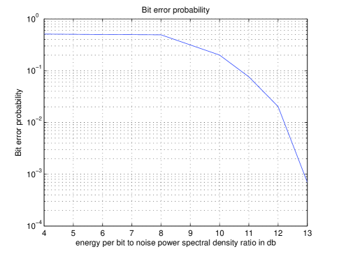
Figure 2: Bit error probabilities for the CM6 channel model. The X-axis shows energy per bit to noise power spectral density ratio $E_{b}/N_{0}$ in dB

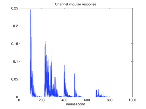
Figure 3: Typical channel impulse response in the CM6 channel model

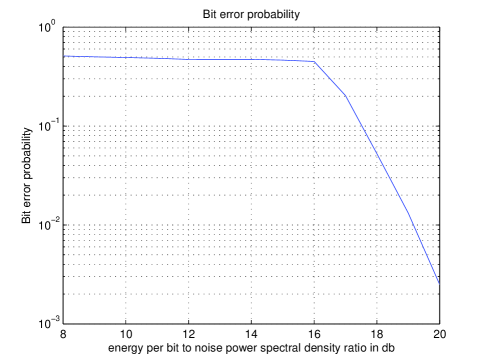
Figure 4: Bit error probabilities for the CM1 channel model. The X-axis shows energy per bit to noise power spectral density ratio $E_{b}/N_{0}$ in dB

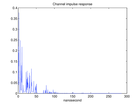
Figure 5: Typical channel impulse response in the CM6 channel model

VI Conclusion

In this paper, we propose an approximate semi-definite programming framework for demodulation and equalization of non-coherent UWB systems with inter-symbol-interference. The proposed algorithm has low computational complexity and storage requirements, which make it an attractive choice for real-time high-speed implementations. Numerical results show that the proposed approach has satisfactory error probability performance. The proposed approach can be adopted in a wide spectrum of non-coherent UWB modulation schemes.

References

[1]
X. Ma, “Reduced complexity demodulation and equalization scheme for
differential impulse radio uwb systems with isi,” in Proc. the IEEE
Sarnoff Symposium, Princeton NJ, March 2009.
[2]
M. Z. Win and R. A. Scholtz, “Ultra-wide bandwidth time-hopping
spread-spectrum impulse radio for wireless multiple-access communications,”
IEEE Transactions on Information Theory, vol. 48, no. 4, pp. 679 –
691, April 2000.
[3]
E. Saberinia and A. H. Tewfik, “Pulsed and nonpulsed OFDM ultra wideband
wireless personal area networks,” in Proc. IEEE Conference on Ultra
Wideband Systems and Technologies (UWBST 2003), Reston, Virginia, USA,
November 2003, pp. 275–279.
[4]
A. Batra, J. Balakrishnan, G. Aiello, J. Foerster, and A. Dabak, “Design of a
multiband OFDM system for realistic UWB channel environments,”
IEEE Transactions on Microwave Theory and Techniques, vol. 52, no. 9,
pp. 2123–2138, September 2004.
[5]
M. Ho, S. Somayazulu, J. Foerster, and S. Ray, “A differential detector for an
ultra-wideband communication system,” in Proc. IEEE Semiannual
Vehicular Technology Conference (VTC Spring 2002), vol. 4, Birmingham, AL,
USA, May 2002, pp. 1896–1900.
[6]
D. Choi and W. Stark, “Performance of ultra-wideband communication with
suboptimal receivers in multipath channels,” IEEE Journal of Selected
Area of Communications, vol. 20, pp. 1754–1766, Dec. 2002.
[7]
S. Mo, N. Guo, J. Zhang, and R. Qiu, “UWB MISO time reversal with energy
detector receiver over ISI channels,” in Proc. IEEE Consumer
Communications and Networking Conference, Las Vegas, Neveda, Jan. 2007, pp.
629–633.
[8]
K. Witrisal, G. Leus, M. Pausini, and C. Krall, “Equivalent system model and
equalization of differential impulse radio UWB systems,” IEEE
Journal on Selected Areas in Communications, vol. 23, no. 9, pp. 1851 –
1862, September 2005.
[9]
E. Hazan, “Sparse approximate solutions to semidefinite programs,” in
Proc. the 8th Latin American Theoretical Informatics Symposium,
Buzios, Rio de Janeiro, Brazil, April 2008.
[10]
S. Boyd and L. Vandenberghe, Convex Optimization. The Edinburgh Building, Cambridge, UK: Cambridge University
Press, 2004.
[11]
E. K. P. Chong and S. H. Zak, An Introduction to Optimization. New York, NY: John Wiley & Sons, Inc, 2001.
[12]
A. F. Molisch, K. Balakrishnan, C.-C. Chong, S. Emami, A. Fort, J. Karedal,
J. Kunisch, H. Schantz, U. Schuster, and K. Siwiak, “Ieee 802.15.4a channel
model - final report,” IEEE, Tech. Rep.
15-04-0662-00-004a-channel-model-final-report-r1, September 2004.