linksLinks

Raymond and Beverly Sackler
Faculty of Exact Sciences
The Blavatnik School of Computer Science

Constructing Two-Dimensional
Voronoi Diagrams via
Divide-and-Conquer of Envelopes
in Space

Thesis submitted in partial fulfillment of the requirements for the M.Sc.
degree in the School of Computer Science, Tel-Aviv University
by
Ophir Setter
This work has been carried out at Tel-Aviv University
under the supervision of Prof. Dan Halperin
May 2009

Acknowledgements

Many people had great influence on this thesis and its author during the research period. I deeply thank my advisor, Prof. Dan Halperin, for his help in guidance, support, and encouragement, and for introducing me the field of applied computational geometry.

I wish to thank Efi Fogel and Eric Berberich for fruitful collaboration and for sharing priceless knowledge. Special thanks are given to Efi for his warm hospitality during fruitful Friday afternoons and for providing the basis for the player software, which enabled the creation of the 3D figures of this thesis. Special thanks are given to Eric for his admirable motivation and for sharing his insights through many rich discussions. I also thank Prof. Micha Sharir for his cooperation and help in theoretical parts of the thesis.

I would also like to thank all other members of the applied computational geometry lab at the computer science school of Tel-Aviv University who provided support and useful suggestions. Special thanks are given to Ron Wein and to Michal Meyerovitch.

I wish to thank all members of the algorithms group at the Max-Planck-Insitut für Informatik in Saarbrücken, Germany, for introducing and helping with the field of computational algebra, and for their hospitality. Special thanks are given to Michael Hemmer, to Eric Berberich, and to Michael Kerber.

Work on this thesis has been supported in part by the Israel Science Foundation (grant no. 236/06), by the German-Israeli Foundation (grant no. 969/07), and by the Hermann Minkowski–Minerva Center for Geometry at Tel Aviv University.

Abstract

We present a general framework for computing two-dimensional Voronoi diagrams of different classes of sites under various distance functions. The framework is sufficiently general to support diagrams embedded on a family of two-dimensional parametric surfaces in ${\mathbb{R}}\rule{0.85358pt}{0.0pt}^{3}$. The computation of the diagrams is carried out through the construction of envelopes of surfaces in 3-space provided by Cgal (the Computational Geometry Algorithm Library). The construction of the envelopes follows a divide-and-conquer approach. A straightforward application of the divide-and-conquer approach for computing Voronoi diagrams yields algorithms that are inefficient in the worst case. We prove that through randomization the expected running time becomes near-optimal in the worst case. We show how to employ our framework to realize various types of Voronoi diagrams with different properties by providing implementations for a vast collection of commonly used Voronoi diagrams. We also show how to apply the new framework and other existing tools from Cgal to compute minimum-width annuli of sets of disks, which requires the computation of two Voronoi diagrams of two different types, and of the overlay of the two diagrams. We do not assume general position. Namely, we handle degenerate input, and produce exact results.

Contents

1. 1 Introduction
2. 2 Preliminaries
   1. 2.1 Voronoi Diagrams
   2. 2.2 Divide-and-Conquer Algorithm for Envelopes
   3. 2.3 CGAL and the Arrangement_on_surface_2 Package
   4. 2.4 Exact Construction of Envelopes in CGAL
3. 3 From Envelopes to Voronoi Diagrams
   1. 3.1 Divide-and-Conquer Algorithm for Voronoi Diagrams
   2. 3.2 Theoretical Aspects
   3. 3.3 Robust Implementation with CGAL
   4. 3.4 Randomizing for Optimality
4. 4 Examples and Implementation Details
   1. 4.1 Planar Voronoi Diagrams
      1. 4.1.1 Voronoi Diagrams with Linear Bisectors
      2. 4.1.2 Voronoi Diagrams with Higher-Degree Algebraic Bisectors
      3. 4.1.3 Voronoi Diagrams with Semi-Algebraic Bisectors
   2. 4.2 Spherical Voronoi Diagrams
      1. 4.2.1 Arrangements of Geodesic Arcs on the Sphere
      2. 4.2.2 Power Diagrams on the Sphere
   3. 4.3 Speeding-up the Computation
5. 5 Discussion: Advantages and Limitations
   1. 5.1 Advantages
   2. 5.2 Limitations
6. 6 Application: Minimum-Width Annulus of Disks
   1. 6.1 Introduction
   2. 6.2 Algorithm for Minimum-Width Annulus of Disks

List of Figures

1. 1.1 Voronoi diagram figure from Descartes research
2. 1.2 Various Voronoi diagrams
3. 3.1 Merging two Voronoi diagrams.
4. 3.2 Worst-case quadratic multiplicatively-weighted Voronoi diagram.
5. 4.1 Computing Voronoi diagrams of points using lower envelopes.
6. 4.2 Voronoi diagrams of points
7. 4.3 Voronoi diagrams of linear objects
8. 4.4 Compare-$u$ predicate implementation
9. 4.5 Geodesic distance function on the sphere.
10. 4.6 Voronoi diagrams on the sphere
11. 4.7 Three-bisectors optimization
12. 5.1 Effect of randomization
13. 5.2 Degenerate Voronoi diagrams
14. 5.3 Farthest-site Voronoi diagrams
15. 5.4 Overlaying an arrangement and a Voronoi diagram on the sphere

Chapter 1 Introduction

In layman’s terms the Voronoi diagram of a given set of objects is the subdivision of the space into regions where each region consists of points that are closer to one particular object than to all others of the given set of objects. Voronoi diagrams are intuitive structures and are even found in various forms in nature. The concept has reappeared in diverse fields of science

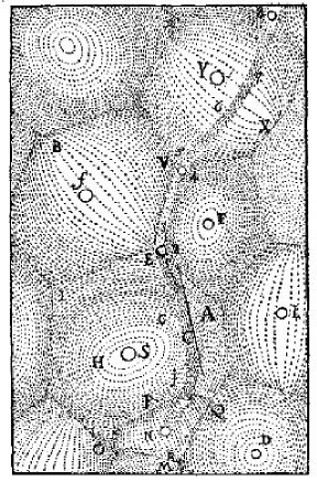
Figure 1.1: A Voronoi diagram figure from a solar system research by Descartes (1644).

throughout history, often receiving a different new name: Wigner-Seitz zones (chemistry and physics), domains of action (crystallography), Thiessen polygons (geography), etc.

Most text books cite a 1644 solar system research by Descartes [d-pp-44] as the first documented application of Voronoi diagrams, even though they were not explicitly defined there. There is no controversy, however, that Dirichlet was the first to formally define the concept of Voronoi diagrams, and that the initial extensive studies on the subject were conducted by him and by Georgy Voronoi [ak-vd-00, obsc-stcavd-00]. This clarifies the fact that the two leading aliases for the diagrams currently are Voronoi diagrams and Dirichlet tessellations. The other most common term refers to the dual diagram to the Voronoi diagram — the Delaunay triangulation (or tessellation). Despite the fact that Voronoi was the first to conceive the dual diagram to the Voronoi diagram, Delaunay was the first to directly define it, earning an alias after his name.

Shamos and Hoey introduced Voronoi diagrams to the field of Computer Science [sh-cpp-75]. They used Voronoi diagrams to improve running times of algorithms for problems, which had been considered unrelated, such as smallest enclosing circle and various closest-point problems. Since then, Voronoi diagrams were thoroughly investigated, and were used to solve many geometric problems.

The concept of Voronoi diagrams, that is, the division of a space into maximally-connected cells, where each cell consists of points that are closer to a particular site than to any other site of a given collection of sites, was extended beyond the scope of point sites and the Euclidean metric [ak-vd-00, bwy-cvd-06, obsc-stcavd-00]. In fact, the original diagram referred to by Descartes (mentioned above) seems more like, what nowadays is called, a weighted Voronoi diagram than a standard Voronoi diagram of points.

The most straightforward generalization of the standard Voronoi diagram is to various kinds of geometric sites while staying in the Euclidean space. These diagrams include Voronoi diagrams of line segments, Voronoi diagrams of circular arcs, Voronoi diagrams of disks in the plane, and Voronoi diagrams of ellipses in the plane.

Different applications impose different types of distance functions to the sites, inducing diverse types of Voronoi diagrams. Among those are: power diagrams of disks, multiplicatively-weighted Voronoi diagrams, and Voronoi diagrams with respect to the $L_{p}$ (Minkowski) and Karlsruhe (Moscow) metrics [obsc-stcavd-00]. Two particularly interesting types of diagrams are the $L_{1}$-diagram of points that can have two-dimensional cells induced by multiple sites (two-dimensional bisectors), and the multiplicatively-weighted Voronoi diagram that can be of quadratic size in the number of input sites.

Voronoi diagrams were also defined in various ambient spaces. For example, Voronoi diagrams defined over different two-dimensional surfaces, such as the Voronoi diagram of points on a sphere, the Voronoi diagram of points on a cone, and the power diagram on a sphere. In higher dimensions the main research efforts concentrated on Voronoi diagrams of point sites and power diagrams, neglecting other types of sites. For example, though the complexity of the Euclidean Voronoi diagram of lines with fixed orientations in three-dimensions was investigated by Koltun and Sharir [ks-tdevd-03], a complete combinatorial and algebraic description of the diagram of three lines was given by Everett et al. [elle-vdtl-07] only recently. In this thesis we concentrate on Voronoi diagrams defined over certain two-dimensional parametric surfaces in 3-space.

Klein unified some classes of planar Voronoi diagrams under a generalized framework by introducing abstract Voronoi diagrams, which are defined in terms of their bisector curves [k-cavd-89, kmm-ricavd-93].

Every type of nearest-site Voronoi diagram defines a complementary farthest-site Voronoi diagram. The farthest-site Voronoi diagram is useful on its own, and one can find applications where both (nearest and farthest) Voronoi diagrams are needed; see Chapter 6. Various farthest-site Voronoi diagrams have nearly-linear time construction algorithms [cg-ps-85, afw-fsgvd-88]. Mehlhorn, Meiser, and Rasch [mmr-fsavd-01] used Klein’s terminology and proved that farthest abstract Voronoi diagrams are of linear size and can be computed with a randomized algorithm in $O(n\log n)$ expected running time.

Algorithms

Numerous approaches for computing Voronoi diagrams were developed. Shamos and Hoey used the divide-and-conquer paradigm to obtain the first optimal $\Theta(n\log n)$-time construction algorithm for the Voronoi diagram of points in the plane [sh-cpp-75]. The algorithm partitions the set of points into two sets of roughly equal size by a vertical line, computes the respective right and left Voronoi diagrams, and finally, carefully merges the two diagrams together. Their main achievement was to prove that there is a polygonal line that “stitches” the two diagrams together (in the merge step), and that it can be found in $O(n)$ time, yielding a $\Theta(n\log n)$-time overall algorithm. A similar approach was used by Klein [k-cavd-89] to supply a $\Theta(n\log n)$-time algorithm for abstract Voronoi diagrams. Guibas and Stolfi described the algorithm in the context of the Delaunay graph (the dual to the Voronoi graph) as a major application for their quad-edge data structure [gs-pmgscv-83]. Dwyer improved the expected running time of the divide-and-conquer algorithm for various point distributions to $O(n\log\log n)$ [d-fdcacd-87].

A different divide-and-conquer approach was recently proposed by Aichholzer et al. [aaahjp-dcvdr-09a]. They employ a divide-and-conquer medial-axis algorithm on an augmented domain to compute the Voronoi diagrams of various types of sites, such as polygonal sites, circular disks, and spline curves. The combinatorial structure of the Voronoi diagram is computed without the construction and manipulation of bisector curves. However, being based on a medial-axis algorithm, their approach supports only diagrams induced by the Euclidean metric.

The ubiquitous sweep-line paradigm, introduced by Bentley and Ottmann [bo-arcgi-79], was adapted by Fortune for the construction of Voronoi diagrams of points in the plane [f-savd-87]. The sweep technique proved useful also for constructing other types of Voronoi diagrams, such as order-$k$ Voronoi diagrams [r-okvdsa-91] and Voronoi diagrams of circles in the Euclidean plane [jkmkh-saevdc-06].

Another important and popular technique is the incremental construction [gs-cdtp-78], which together with randomization [cs-arscg-89] yield an $O(n\log n)$ algorithm for constructing Voronoi diagrams [gks-ricdvd-92]. This technique was used to attain algorithms for various types of Voronoi diagrams, and allowed relaxation of certain requirements on bisector curves in the definition of abstract Voronoi diagrams, while keeping an optimal time complexity [ky-vdpco-03, kmm-ricavd-93].

Lower or upper envelopes of surfaces constitute a fundamental structure in computational geometry. They are frequently used to solve various problems including: hidden surface removal, computing Hausdorff distances, and more [as-ata-00, sa-dssga-95]. Agarwal et al. presented an efficient and simple divide-and-conquer algorithm for constructing envelopes in three dimensions [ass-olea-96]. The theoretical worst-case time complexity of constructing the envelope of $n$ “well-behaved” surfaces in three dimensions using the divide-and-conquer algorithm is $O(n^{2+\varepsilon})$. This near-quadratic running time can arise also in cases of envelopes of linear complexity. This is also an upper bound, almost tight in the worst case, on the combinatorial complexity of the envelope.

Edelsbrunner and Seidel [es-vda-86] observed the connection between Voronoi diagrams in ${\mathbb{R}}\rule{0.85358pt}{0.0pt}^{d}$ and lower envelopes of the corresponding distance functions to the sites in ${\mathbb{R}}\rule{0.85358pt}{0.0pt}^{d+1}$, yielding a very general approach for computing Voronoi diagrams. For example, consider the Voronoi diagram of a set of points in the plane, then, the connection is as follows: for each point site $p=(x_{p},y_{p})$ we consider the paraboloid $P_{p}(x,y)=(x-x_{p})^{2}+(y-y_{p})^{2}$. The minimization diagram of the lower envelope of the paraboloids, which is the vertical projection of the lower envelope onto the plane, corresponds to the Voronoi diagram of the points.

Other algorithms include Yap’s algorithm for segments and circular arcs [y-avdssc-87], an optimal algorithm for the construction of weighted Voronoi diagrams [ae-oacwvd-84]. The interested reader is referred to the book by Okabe et al. [obsc-stcavd-00] and to the survey by Aurenhammer and Klein [ak-vd-00] for more information.

Software

The Computational Geometry Algorithms Library (Cgal)cgal-link is an open-source C++ library of efficient and reliable geometric algorithms. It follows the exact geometric computation paradigm [y-rgc-04, yd-ecp-95] to achieve robustness with exact results. Cgal contains implementations of algorithms for computing the dual Delaunay graphs to standard Voronoi diagrams, Apollonius diagrams, and segment Voronoi diagrams [bdpty-tic-02, ek-padaai-06, k-reisvd-04]. Moreover, Voronoi diagrams of ellipses can be computed using the same Cgal framework [ett-vdec-08]. Other exact implementations include the construction of segment Voronoi diagrams in Leda [bms-hcvdls-94] and the implementation of the randomized algorithm for constructing abstract Voronoi diagrams in Leda [s-eiavd-94].

Approximated alternatives include the Vroni code for computing two-dimensional Voronoi diagrams of points and line segments [h-vearec-01], the use of the Graphics Processing Unit (GPU) to visualize Voronoi diagrams [hklmc-fcgvd-99, n-itvdg-08], and more.

A large number of the implementations for constructing Voronoi diagrams use the incremental construction paradigm. The time complexity achieved by the incremental construction relies on the fact that most changes applied to the diagram are local with respect to the location of the inserted site. This assumption usually implies that the diagrams are of linear size. Typically, the time complexity of constructing a Voronoi diagram that has linear complexity, using the above algorithms, is nearly linear.

One of the main packages included in Cgal is the Arrangement_on_surface_2 package, which supports construction and maintenance of arrangements of bounded or unbounded curves embedded on certain two-dimensional parametric surfaces in three-dimensions and different operations on them [cgal:wfzh-a2-08, wfzh-aptaca-07, bfhmw-smtdas-07]. The Arrangement_on_surface_2 package is robust when using exact arithmetic and handles all degenerate input.

Cgal contains a robust and efficient implementation of the divide-and-conquer algorithm mentioned earlier for constructing envelopes of surfaces in three dimensions [cgal:mwz-e3-08, m-rgeces-06]. The implementation, provided in Cgal’s Envelope_3 package, relies heavily on arrangements and algorithms from the Arrangement_on_surface_2 package. As mentioned above, the divide-and-conquer algorithm achieves a worst-case near-quadratic running time. This fact poses an obstacle when attempting to utilize this algorithm for the construction of Voronoi diagrams that have linear complexity, as we aim for algorithms that run in near-linear time.

Contribution of the Thesis

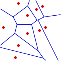
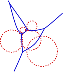
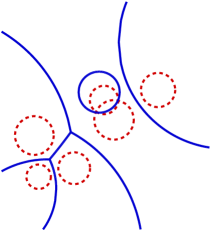
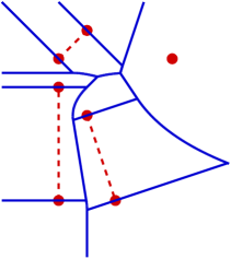
Figure 1.2: Various Voronoi diagrams computed with our software. (For the parameters of sites in each diagram, see Table 1.1.) 1.2 A standard Voronoi diagram (point sites with $L_{2}$ metric). 1.2 An additively-weighted Voronoi (Apollonius) diagram with disk centers as sites and disk radii as weights. 1.2 A Möbius diagram with disk centers as sites. The distance from every point on the boundary of a disk to its corresponding site is zero. 1.2 A Voronoi diagram of segments and points. The sites in 1.2, 1.2, and 1.2 are illustrated with dashed curves. The figures in this thesis are best viewed in color.

We present a general framework for constructing various two-dimensional Voronoi diagrams, exploiting the efficient, robust, and general-purpose envelope code of Cgal. We have extended the Envelope_3 package to work together with the new Arrangement_on_surface_2 package and created spherical geodesic Voronoi diagrams based on our self-developed code for constructing arrangements of geodesic arcs on the sphere. The work in this context was presented at the $24^{th}$ European Workshop on Computational Geometry [fsh-eiaga-08] and in the multimedia session of the $24^{th}$ Annual Symposium on Computational Geometry [fsh-agas-08]; for more information on the computation of arrangements of geodesic arcs on the sphere and applications see Efi Fogel’s thesis [f-mscaag-08].

Table 1.1: Types of Voronoi diagrams currently supported by our implementation, and their bisector classes.

Name	Sites	Distance function	Class of bisectors
Standard Voronoi diagram	points $p_{i}$	$||x-p_{i}||$	lines
Power diagram	disks (with center $c_{i}$ and radius $r_{i}$)	$\sqrt{(x-c_{i})^{2}-r_{i}^{2}}$
2-point triangle-area Voronoi diagram	pairs of points $\{p_{i},q_{i}\}$	area of $\triangle xp_{i}q_{i}$	pairs of lines
Apollonius diagram	points $p_{i}$ and weights $w_{i}$	$||x-p_{i}||-w_{i}$	hyperbolic arcs
Möbius diagram	points $p_{i}$ with scalars $\lambda_{i},\mu_{i}$	$\lambda_{i}(x-p_{i})^{2}-\mu_{i}$	circles and lines
Anisotropic diagram	points $p_{i}$, with positive definite matrices $M_{i}$, and scalars $\pi_{i}$	$(x-p_{i})^{t}M_{i}(x-p_{i})-\pi_{i}$	conic arcs
Voronoi diagram of linear objects	interior-disjoint points, segments, rays, or lines	Euclidean distance	piecewise algebraic curves composed of line segments and parabolic arcs
Spherical Voronoi diagram	points on a sphere	geodesic distance	arcs of great circles (geodesic arcs)
Power diagram on a sphere	circles on a sphere	“spherical” power distancea

• Given a point $p$ and a circle with center $q$ and radius $r$ on the sphere, the spherical power “proximity” between $p$ and the circle is defined to be $\frac{\cos{d(p,q)}}{\cos{r}}$ where $d(p,q)$ is the geodesic distance between $p$ and $q$ [s-lvds-02].

Chapter 2 gives the necessary background and basic definitions. Chapter 3 describes the adaptation of the divide-and-conquer algorithm for envelopes to Voronoi diagrams embedded on two-dimensional parametric surfaces in 3-space, and the elimination of the above complexity obstacle using randomization in the divide step. We describe the software interface between the construction of Voronoi diagrams and the envelope code of Cgal. An analysis by Micha Sharir for the expected time complexity of constructing lower envelopes in this randomized divide-and-conquer setup can be found in Section 3.4. Chapter 4 presents details about our implementation of a large set of Voronoi diagrams with different properties using our framework. The section demonstrates the generality of the framework and gives information on techniques we have applied to speed-up the exact (and costly) computation in practice. Table 1.1 summarizes the types of diagrams that are currently supported by our implementation. In Chapter 5, we thoroughly discuss the advantages and the limitations of our framework. We also show experimental results, demonstrating the randomization effect on the running time. We present an application of our framework to solve the problem of computing a minimum-width annulus of a set of disks in the plane, which exploits the generality and the flexibility of the framework in Chapter 6; a short introduction to the minimum-width annulus problem is given in Section 6.1. The solution requires the computation of two Voronoi diagrams of two different types, and of the overlay of the two diagrams. We presented an extended abstract of this work of computing a minimum-width annulus of disks at the $25^{th}$ European Workshop on Computational Geometry [sh-ecmwad-09]. An extended abstract of the thesis will be presented on the $6^{th}$ annual International Symposium on Voronoi Diagrams in science and engineering (ISVD) [ssh-ctdvd-09].

The major strength of our approach is its completeness, robustness, and generality, that is, the ability to handle degenerate input, the agility to produce exact results, and the capability to construct diverse types of Voronoi diagrams. The code is designed to successfully handle degenerate input, while exploiting the synergy between generic programming and exact geometric computing, and the divide-and-conquer framework to construct Voronoi diagrams. Theoretically, the randomized divide-and-conquer envelope approach for computing Voronoi diagrams is efficient and it is asymptotically comparable to other (near-)optimal methods. However, the method uses constructions of bisectors and Voronoi vertices as elementary building blocks, and they must be exact, which makes the concrete running time of our exact implementation inferior to those of existing implementations of various dedicated (specific diagram type) implementations.

Our software can support practically any kind of Voronoi diagrams, provided that the user supplies a set of basic procedures for manipulating a small number of sites and their bisectors (see Section 3.3 and Chapter 4 for details on how to use the framework to compute new types of Voronoi diagrams.) Figure 1.2 illustrates several types of planar Voronoi diagrams computed by our software. The figure above shows two types of Voronoi diagrams on the sphere computed with our software; its left part shows a spherical Voronoi diagram of 14 points and its right part shows a spherical power diagram of 10 circles. Both diagrams are composed of geodesic arcs.

Cgal had a significant impact on this thesis. All the software components involved in this thesis are based on Cgal and are developed according to its guidelines. The developed software adheres to the generic programming paradigm and follows the exact geometric computation paradigm, similar to other existing Cgal components. Nonetheless, this thesis also had an influence on Cgal. The results of this thesis contributed to Cgal in the form of improving existing components and in developing new components that are planned to be integrated into a future public release of Cgal. This includes, for example, contributing to the development of the new Arrangement_on_surface_2 package, extending the Envelope_3 package to support envelopes embedded on two-dimensional surfaces, and enhancing existing traits classes for the arrangement package and the arrangement package itself. The code presented in this thesis is packed into a package, in the form of a Cgal package, named EnvelopeVoronoi_2.

Chapter 2 Preliminaries

This chapter provides background material and definitions required for the understanding of this thesis. Sections 2.1 and 2.2 provide general definitions for Voronoi diagrams and describe the divide-and-conquer algorithm for constructing envelopes of surfaces in three-dimensions. Basic software components and technical background, the implementations included in this thesis are built upon, are reviewed in Sections 2.3 and 2.4.

2.1 Voronoi Diagrams

Let $O=\{o_{1},\ldots,o_{n}\}$ be a set of $n$ objects, referred to as Voronoi sites, in an ambient space $\mathcal{S}$. Let $\rho:O\times\mathcal{S}\to{\mathbb{R}}\rule{0.85358pt}{0.0pt}$ be a distance function between Voronoi sites and points in the space. The Voronoi diagram ${\rm Vor}_{\rho}(O)$ of the set $O$ with respect to the distance function $\rho$ is defined to be the partition of the space $\mathcal{S}$ into maximally connected cells, where each cell consists of points that are closer to one particular site (or a set of sites) than to any other site. Formally, every point $p\in\mathcal{S}$ lies in a cell corresponding to a set of sites $I\subseteq O$ if, and only if, $\rho(o_{i},p)<\rho(o_{j},p)$ for every $o_{i}\in I,o_{j}\notin I$, and $\rho(o_{i},p)=\rho(o_{j},p)$ for every $o_{i},o_{j}\in I$. Likewise, the farthest Voronoi diagram is the partition of the space into maximally connected cells, where each cell consists of points that are farther from one site than from the other sites.

All Voronoi diagrams can be defined by adjusting the parameters $O$, $\rho$, and $\mathcal{S}$ as required. Defining the standard Voronoi diagram, for example, amounts to the selection of a set of points in the plane as the set of sites, the selection of the plane itself as the ambient space, and the selection of the Euclidean distance between two points in the plane as the distance function. The power diagram on the sphere, yet another example, is defined by choosing $O$ to be a set of circles on the unit sphere, $\mathcal{S}$ to be the sphere, and $\rho$ to be the spherical power distance.

In certain cases, the distance to a site may depend on various parameters associated with the site. For example, Möbius diagrams’ distance depends on two positive scalars, and anisotropic Voronoi diagrams’ distance depends on one positive definite matrix and one positive scalar. Table 1.1 lists some of the more prevalent two-dimensional Voronoi diagrams together with their respective types of sites, ambient spaces, and distance functions.

The bisector $B(o_{i},o_{j})$ of two Voronoi sites $o_{i}$ and $o_{j}$ is the locus of points that have an equal distance to both sites, that is

$$B(o_{i},o_{j})=\{p\in\mathcal{S}\mid\rho(o_{i},p)=\rho(o_{j},p)\}.$$

From here on we refer only to ambient spaces that are two-dimensional, parameterizable, and orientable (e. g., a plane, a sphere, a torus, etc.)

The above definition is the more classical definition conceived from the need to divide the space into areas of influence or dominance. The sites are, of course, the dominating entities and the distance functions correspond to the measure of dominance of each site on points of the ambient space. In addition to this application-inspired definition an alternative implementation-oriented definition arose.

Considering the plane as the ambient space, Voronoi diagrams were defined through their bisecting curves instead of the distance function. Such diagrams that also comply to additional restrictions are referred to as abstract Voronoi diagrams [k-cavd-89]. In this definition, a set $B$ is called a bisecting curve if, and only if, $B$ is homeomorphic to the open interval $(0,1)$ and closed as a subset of ${\mathbb{R}}\rule{0.85358pt}{0.0pt}^{2}$. A bisecting curve $B$ partitions the plane into two unbounded areas. For each pair of sites $o_{i}$ and $o_{j}$ we assume that $B(o_{i},o_{j})=B(o_{j},o_{i})$ is a bisecting curve, and denote by $D(o_{i},o_{j})$ and $D(o_{j},o_{i})$ the two areas obtained in the partition induced by the bisecting curve. (One of the areas is known to be $D(o_{i},o_{j})$ and one is known to be $D(o_{j},o_{i})$.) The Voronoi diagram ${\rm Vor}(O)$ is defined as follows:

$${Reg}{}(o_{i},o_{j}) = \left\{\begin{array}[]{ll}D(o_{i},o_{j})\cup B(o_{i},o_{j}),&\text{if $i<j$}\\ D(o_{i},o_{j})&\text{if $i>j$}\end{array}\right.$$ (2.3)

$${Reg}{}(o_{i},O) = \bigcap_{o_{j}\in O,j\neq i}{Reg}{}(o_{i},o_{j})$$ (2.4)

$${\rm Vor}(O) = \bigcup_{o_{i}\in O}\partial{Reg}{}(o_{i},O)$$ (2.5)

Abstract Voronoi diagrams do not cover the entire variety of Voronoi diagrams discussed in this thesis. For example, Möbius diagrams and anisotropic diagrams are not abstract Voronoi diagrams. In addition, the classical definition of abstract Voronoi diagrams does not include the cases of different ambient spaces, such as two-dimensional parametric surfaces.

2.2 Divide-and-Conquer Algorithm for Envelopes

Given a set of bivariate functions (partially) defined over a two-dimensional domain $\mathcal{S}$, $\mathcal{F}{}=\{f_{1},\ldots,f_{n}\}$, $f_{i}:~{}\mathcal{S}{}~{}\to~{}{\mathbb{R}}\rule{0.85358pt}{0.0pt}$, its lower envelope ${\mathcal{E}}_{\mathcal{F}}:~{}\mathcal{S}{}~{}\to~{}{\mathbb{R}}\rule{0.85358pt}{0.0pt}$ is defined to be their point-wise minimum:

$${\mathcal{E}}_{\mathcal{F}}(x)=\min_{i}f_{i}(x).$$

The minimization diagram ${\mathcal{M}}_{\mathcal{F}}$ of $\mathcal{F}$ is the subdivision of $\mathcal{S}$ into maximal relatively-open connected cells, such that the function (or the set of functions) that attains the lower envelope over a specific cell of the subdivision is the same. Changing “$\min$” to “$\max$” in the definition above results in the corresponding definitions for upper envelope and maximization diagram.

Agarwal, Schwarzkopf, and Sharir presented a simple and efficient divide-and-conquer algorithm for the construction of envelopes of bivariate functions defined over the plane [ass-olea-96]. The algorithm is essentially an application of the overlay of two-dimensional minimization diagrams. They showed that the combinatorial complexity of such an overlay of two envelopes of $n$ “well-behaved” functions is $O(n^{2+\varepsilon})$; see [as-ata-00] for a full description of the assumptions on such functions. An alternative proof was given by Koltun and Sharir [ks-ptoe-03]. As acceptable in the field of computational geometry they assumed that the input is given in general position. This assumption creates a gap between the theoretical divide-and-conquer algorithm for constructing envelopes in three-dimensions and its practical anticipated implementation.

Meyerovitch presented an implementation for the above algorithm for constructing envelopes of functions defined over the plane [m-rgeces-06, m-rgeces-thesis-06], which handles all inputs, including all degenerate situations; see more details in Section 2.3 below. Following is a description of the algorithm in the context of lower envelopes construction. The description is easily adapted to the case of upper envelopes as well. The input for the algorithm is a set $\mathcal{F}$ of bivariate functions, which could be partially defined, and the result is the minimization diagram ${\mathcal{M}}_{\mathcal{F}}$ of the set of functions.

The envelope of a single function comprises the function itself. Hence, the minimization diagram is constructed by projecting the boundary of the domain of the function onto ${\mathbb{R}}\rule{0.85358pt}{0.0pt}^{2}$. In the case where the set of functions consists of more than one function we partition the set into two sets of functions of roughly equal size $\mathcal{F}{}_{1}$ and $\mathcal{F}{}_{2}$, and compute their respective minimization diagrams ${\mathcal{M}}_{1}$ and ${\mathcal{M}}_{2}$, recursively. Every feature — a vertex, an edge, or a face — of ${\mathcal{M}}_{1}$ and ${\mathcal{M}}_{2}$ is labeled with the set of functions that attain the lower envelope over it. We merge ${\mathcal{M}}_{1}$ and ${\mathcal{M}}_{2}$ into the final minimization diagram ${\mathcal{M}}_{\mathcal{F}}$. The merge operation is composed of three stages:

1. Overlaying ${\mathcal{M}}_{1}$ and ${\mathcal{M}}_{2}$ each represented as a planar arrangement to obtain a new planar arrangement. We use a sweep-based overlay algorithm, during the execution of which new features are created depending on existing features of both input diagrams; for example, a new vertex is created by overlaying two intersecting edges from ${\mathcal{M}}_{1}$ and ${\mathcal{M}}_{2}$, respectively. The newly created features are labeled with references to the functions attaining the lower envelopes over both input minimization diagrams.

2. Constructing the minimization diagram over every feature (the vertices, the edges, and the faces) of the overlay.

   If the overlaid features from both minimization diagrams that induce the subject feature reference no functions then the feature is labeled with the empty set. If only one feature references a set of functions then the subject feature is labeled with this set of functions.

   The case where both input features reference sets of functions makes our task a non-trivial one, as we may have to split the feature into several pieces (if it is an edge or a face). All referenced functions originating from a single minimization diagram are identified over the subject feature, so we can consider one representative function from each of the diagrams (${\mathcal{M}}_{1}$ and ${\mathcal{M}}_{2}$). The projected intersection between these two functions induces the split of the feature into fragments. Each of the resulting fragments is then labeled with the correct set of functions according to the value obtained by the functions over it (the set of functions originating from ${\mathcal{M}}_{1}$ or ${\mathcal{M}}_{2}$ in case one set obtains a lower value, or the union of both sets in case they obtain an equal value).

3. Removing redundant features. Neighboring faces in the refined overlay and their connecting edges can be labeled with identical sets of functions. If this is the case we compute the union of the redundant faces by removing edges and vertices, which yields the final minimization diagram.

Assuming that all functions are “well-behaved” (see, e. g., [as-ata-00]), the complexity of the algorithm is dependant on the complexity of the overlay of the two minimization diagrams. Therefore, the theoretical worst-case time-complexity for constructing envelopes using the divide-and-conquer algorithm is $O(n^{2+\varepsilon})$. The actual implementation in Cgal, presented in Section 2.4, contains speed-ups that expedite the practical running time.

2.3 CGAL and the Arrangement_on_surface_2 Package

Providing robust, efficient, and general implementations of computational geometry algorithms is a notoriously difficult task. Two prime issues bring up the majority of difficulties.

The first is the general hardship of implementing geometric algorithms while considering all kinds of degenerate input and boundary situations. Assuming that the given input is in general position is used to avoid these marginal cases in many geometric algorithms in theory. The assumption of general position suggests that special or “coincidental” inputs be discarded; for example, three lines in the plane are assumed not to intersect at a single point. This discards many cases that appear in practical applications and real-world problems, and creates a large gap between computational-geometry algorithms in theory and their implementation.

The second issue is related to robustness and rounding errors. Geometric algorithms in theory generally follow a computational model named “real RAM” [cg-ps-85]. They assume that all numerical computations are performed with unlimited precision, and require constant time per operation. In reality this model cannot be realized. Numbers represented by machines either have limited precision, or require more than constant time per operation, as native types comprise a fixed number of bits. Inaccurate numerics can impose inconsistent predicates and constructions, forming unstable geometric algorithms [kmpsy-cerpg-08]. Developing a robust and efficient geometric algorithm under these constraints is a very challenging task even for a qualified professional.

Cgal, the Computational Geometry Algorithms Library, was launched in 1996 as a collaborative effort of several research institutes in Europe and Israel to provide easy access to efficient, robust, and reliable geometric algorithms and data structures for academic and industrial use.

Cgal provides various geometric data structures and algorithms like convex hull algorithms, Delaunay triangulations, Voronoi diagrams, Boolean operations on polygons and polyhedra, arrangements of curves, Minkowski sums of polygons, alpha shapes, search structures, and more [cgal:eb-08]cgal-link. Cgal is used in various fields in academia and industry, such as computer graphics, scientific visualization, computer-aided design, bioinformatics, motion planning, and more.

Cgal overcomes the above difficulties by adhering to the exact geometric computation paradigm [yd-ecp-95], and by relying on computation with exact number types to achieve robustness. Cgal adheres to the generic programming paradigm (see below) to achieve maximum flexibility without compromising efficiency.

Generic programming is a programming discipline in which concrete algorithms are gradually lifted over specific required types by describing them in terms of polymorphic abstract types [a-gps-99]. The types are provided later at instantiation time of the algorithm as parameters. This approach empowers the programmer with the ability to write dynamic and general programs on abstract types, at the expense of code tangibility. Collections of requirements from abstract polymorphic types are referred to as concepts, and specific types used to instantiate the algorithms are referred to as models.

Templates (or template programming) are C++ language constructs that were designed to support the generic programming paradigm. They have been found to be extremely useful, providing C++ programmers with the ability to write static code-generators and perform static computations (meta-programming), which improves the run-time of non-templated C++ compiled code while maintaining and even enhancing flexibility. In fact, C++ can be regarded as a two-level language where each level is Turing-complete; the first level is the code-generating statically-expanding compile-time consuming template declarations and meta-programs, and the second level is the “standard” non-templated runtime-consuming code. For an in-depth discussion of C++ templates we refer the reader to “C++ Templates” by Vandevoorde and Josuttis [vj-ct-02] and to “Modern C++ Design” by Alexandrescu [a-mcd-01].

Cgal is divided into packages, where each package provides an efficient implementation of a geometric algorithm (or a family of algorithms) or a useful data-structure, and related functionalities. Cgal packages are organized in three parts. Geometric data-structures and algorithms, as just mentioned, are one part. These data structures and algorithms operate on geometric objects like points and segments, and perform geometric tests on them. The objects and predicates are regrouped in Cgal “Kernels”, which constitute another part of Cgal. The third part of Cgal is the “Support Library” which offers fundamental utilities used throughout Cgal; for example, various extensions for the STL stl-link, Boost boost-link and QT libraries.

The support library also contains classes that represent numbers, referred to as “number types,” which are used as parameters to Cgal kernel classes. Depending on the problem (and the input) to be handled, the number types provide a trade-off between efficiency and accuracy. For example, in some cases the user is able to instantiate a geometric kernel with a built-in number-type of C++ that represent a discrete (bounded) subset of the rational numbers, while in other cases he/she has to use a number type that supports all operations in unlimited precision over the rationals, such as the rational number type CGAL::Gmpq based on Gmp— Gnu’s Multi Precision library gmp-link.

A leading package of Cgal — both in terms of size (lines of code) and the extent of usage — is the Arrangement_on_surface_2 package. Given a set $\mathcal{C}$ of curves embedded on a given two-dimensional surface, the arrangement $\mathcal{A}$($\mathcal{C}$) is the subdivision of the surface into cells, induced by the curves of $\mathcal{C}$. Arrangements are defined more generally [bfhmw-smtdas-07]. However, we restrict ourselves here to 2D arrangements, which are supported by Cgal.

The Arrangement_on_surface_2 package is based on the earlier Arrangement_2 package that supported planar arrangements of bounded and unbounded curves [fwh-cfpeg-04, wfzh-aptaca-07]. The Arrangement_on_surface_2 package enables the user to construct and maintain arrangements embedded on certain two-dimensional orientable parametric surfaces [bfhmw-smtdas-07]. In addition to the ability to construct arrangements, the package supports various operations on arrangements, including traversing an arrangement, performing point-location queries on an arrangement, and overlaying two arrangements [cgal:wfzh-a2-08].

The arrangement package of Cgal achieves robustness and exact results when using exact arithmetic types, and handles all kinds of degenerate situations. It supports two algorithmic frameworks, that is the sweep-line framework and the zone-computation framework. Both are used in various geometric algorithms. For example, the former is used for Boolean-set operations between linear or general polygons in the plane, and the latter is used for inserting a curve into an existing arrangement of curves.

The arrangement package follows the generic programing paradigm through the use of traits classes, which enable the separation of the geometric and the topological aspects of the computation. Models that describe behaviors are referred to as traits classes [m-tnutt-97]. A traits class is passed as a parameter to a templated method or a class template and should provide certain predefined types and methods that enable the operation of a specific algorithm. For example, in our case, a geometry traits class for the Arrangement_on_surface_2 class (see below) should contain types that represent points and $x$-monotone curves, a method to compare the $x$-coordinates of two points, etc. This decouples the implementation of the algorithms contained in the Arrangement_on_surface_2 package from the specific geometric computations, and enables the user of the package to create different types of arrangements for different classes of curves.

The main class of the package — Arrangement_on_surface_2 — is parameterized with two template classes, a geometry-traits class and a topology-traits class. The geometry-traits class controls the geometric aspects of the arrangement, namely, it defines associated geometric types (points, curves, and $x$-monotone curves) for the specific family of curves and provides the arrangement with required geometric operations and predicates on those types (e. g., intersecting two $x$-monotone curves, determining whether a point lies below or above a curve, etc.). The topology-traits class, as its name suggests, is responsible for the topological (abstract, graph-like) representation of the arrangement, namely, keeping the correct relations between the arrangement’s cells (faces, edges, and vertices) and their neighboring cells with respect to the embedding surface.

The package is designed for maximum efficiency and flexibility, where flexibility refers to both adaptability and extensibility. In other words, the arrangement package was designed to have the ability to be incorporated into existing user code and the ability to be enhanced with additional code.

2.4 Exact Construction of Envelopes in CGAL

The Envelope_3 package, which implements the algorithm mentioned in Section 2.2 for computing the lower (or the upper) envelope of a set of surfaces in three-dimensions [cgal:mwz-e3-08], is strongly built-upon the Arrangement_2 package. There is one difference between the description of the algorithm in Section 2.2 and the implementation of the Envelope_3 package, that is, the support of Envelope_3 in constructing the envelope of general three-dimensional surfaces by the decomposition of the surfaces into bivariate (partially defined) functions. The package decouples the topology-related computation from the geometry-related computation, making its code generic and easy to reuse and adapt.

The code insures stability, namely, it handles all possible degenerate situations in the case of general surfaces; among those are vertical surfaces, overlapping (and partially overlapping) surfaces, and a common intersection point of more than three surfaces. While insuring stability, the number of calls to the exact (and slow) geometric predicates is minimized by propagating pre-computed information about the structure of the envelope to neighboring cells in the merge step of the algorithm.

The Envelope_3 package defines a new concept for a traits class for computing envelopes of surfaces in three-dimensions. The EnvelopeTraits_3 refines the ArrangementTraits_2 concept, adding types and predicates that are used to compute envelopes. Every model of the EnvelopeTraits_3 has to supply the ability of constructing an arrangement from the projected intersection curves and boundary curves of the given surfaces. Available traits classes for the Envelope_3 package include traits classes for computing the envelopes of triangles, spheres, planes, and quadrics [bm-ceq-07, m-rgeces-06].

The implementation mainly makes use of two operations supported by the arrangement package: (i) sweep-based overlay operation, which is used to overlay two minimization diagrams, and (ii) zone computation-based insertion operation, which is used to insert projected intersection curves (of the surfaces) that partition cells of the refined arrangement. The new Arrangement_on_surface_2 package extends the aforementioned operations, that is, the sweep-line and zone-computation, to support arrangements on two-dimensional parametric surfaces. Thus, we extended the Envelope_3 code to work together with the new Arrangement_on_surface_2 package, and handle minimization diagrams that are embedded on two-dimensional parametric surfaces.

Though computing lower envelopes of functions defined over two-dimensional orientable parametric surfaces has its own significance, we concentrate on describing how this ability is exploited to compute Voronoi diagrams on surfaces; see Section 3.3 for more details and Section 4.2 for a concrete example of computing Voronoi diagrams on the sphere.

Chapter 3 From Envelopes to Voronoi Diagrams

This chapter describes the adaptation of the algorithm for constructing envelopes of bivariate functions to the computation of general Voronoi diagrams. Section 3.1 describes the way the algorithm works in the context of Voronoi diagrams. Section 3.2 discusses theoretical aspects of the algorithm. It shows that through randomization, the expected running time of the algorithm is near-optimal in the worst case. Section 3.3 provides comprehensive details on the software interface that allows the computation of general two-dimensional Voronoi diagrams through the construction of envelopes in Cgal.

3.1 Divide-and-Conquer Algorithm for Voronoi Diagrams

There is a strong connection between Voronoi diagrams in $d$-dimensions and envelopes of functions in $(d+1)$-dimensions, which was first observed by Edelsbrunner and Seidel [es-vda-86]. Their main revelation was the relation between Euclidean Voronoi diagrams of point-sets in ${\mathbb{R}}\rule{0.85358pt}{0.0pt}^{d}$ (and their higher-order Voronoi diagrams) to arrangements of hyperplanes in ${\mathbb{R}}\rule{0.85358pt}{0.0pt}^{d+1}$, which yielded a very general approach for computing various types of Voronoi diagrams.

We demonstrate the connection between Voronoi diagrams and envelopes in the planar case. This connection can be easily established also for two-dimensional parametric surfaces as the embedding spaces. Let $O=\{o_{1},\ldots,o_{n}\}$ be a set of $n$ Voronoi sites in the plane, and let $\rho:O\times{\mathbb{R}}\rule{0.85358pt}{0.0pt}^{2}\to{\mathbb{R}}\rule{0.85358pt}{0.0pt}$ be a distance function between Voronoi sites and points in the plane. Recalling the definitions of Voronoi diagrams and envelopes from Section 2.1 and Section 2.2, it is clear that if we define $f_{i}:{\mathbb{R}}\rule{0.85358pt}{0.0pt}^{2}\to{\mathbb{R}}\rule{0.85358pt}{0.0pt}$ to be $f_{i}(x)=\rho(o_{i},x)$, for each $i=1,\ldots,n$, then the minimization diagram of $\{f_{1},\ldots,f_{n}\}$ corresponds to the Voronoi diagram of $O$. Likewise, the respective maximization diagram corresponds to the farthest Voronoi diagram of $O$.

As we aspire to use envelopes to compute Voronoi diagrams, we “translate” below the terms used in envelopes construction to terms used in Voronoi diagrams computation. This translation will be useful in Section 3.3 where we define the interface for computing Voronoi diagrams. The interface is simpler than the given Cgal interface for computing envelopes. This allows the user of our framework to create a new type of Voronoi diagrams by providing certain functions and types without the knowledge of the underlying envelope algorithm.

Each Voronoi site is transformed into a bivariate function defined over the whole two-dimensional domain, as opposed to envelopes of general surfaces that can be partially defined. The bisector of two Voronoi sites is the locus of points that have an equal distance to both sites (see Section 2.1), thus, the projection of the intersection between two functions that correspond to two Voronoi sites is the bisector of the two sites.

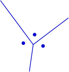
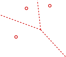
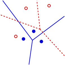
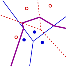
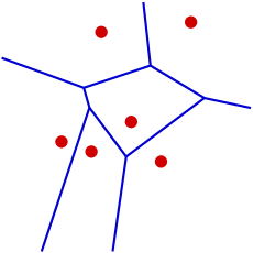
Figure 3.1: The merge step of the divide-and-conquer algorithm for computing Voronoi diagrams. (a) The first Voronoi diagram, ${\rm Vor}_{\rho}(S_{1})$. (b) The second Voronoi diagram, ${\rm Vor}_{\rho}(S_{2})$. (c) The overlay of the two diagrams. (d) The refined overlay. Each face is partitioned to regions that are closer to sites from $S_{1}$ and region that are closer to sites from $S_{2}$. (e) The final diagram obtained after the removal of redundant features from the refined overlay.

The adapted algorithm for Voronoi diagrams computation follows. We split the set of sites into two disjoint subsets $S_{1}$ and $S_{2}$ of (roughly) equal size, construct their respective Voronoi diagrams ${\rm Vor}_{\rho}(S_{1})$ and ${\rm Vor}_{\rho}(S_{2})$, recursively, and then merge the two diagrams to obtain ${\rm Vor}_{\rho}(S)$.

The merge step begins with overlaying the two diagrams. For each face $f$ of the overlay, all its points have a fixed pair of nearest sites $s_{1}$ and $s_{2}$ from $S_{1}$ and $S_{2}$, respectively, where the bisector between $s_{1}$ and $s_{2}$ (restricted to $f$) partitions $f$ into its portion of points nearer to $s_{1}$ and the complementary portion of points nearer to $s_{2}$. This results with portions of the final Voronoi cells. Each feature of the refined overlay is labeled with the sites nearest to it.

Finally, redundant features are removed and subcells of the same cell are stitched together, to yield the combined final diagram. Figure 3.1 illustrates the process of merging two Voronoi diagrams of points (a red one and a blue one), to yield the final Voronoi diagram of the unified set of points.

3.2 Theoretical Aspects

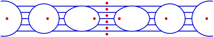
Figure 3.2: A worst-case quadratic-size example of a multiplicatively-weighted Voronoi diagram with 12 sites, based on an example of Aurenhammer and Edelsbrunner [ae-oacwvd-84]. The diagram was computed with our software.

Recall that the asymptotic worst-case time complexity of the divide-and-conquer envelope algorithm (under the natural assumption that the functions have “constant description complexity”) is $O(n^{2+\varepsilon})$, for any $\varepsilon>0$. Indeed, there are planar Voronoi diagrams that obtain quadratic complexity, and for which this construction is nearly worst-case optimal. For example, Figure 3.2 illustrates the worst-case behavior of multiplicatively-weighted Voronoi diagrams, based on an example by Aurenhammer and Edelsbrunner [ae-oacwvd-84]. However, for cases where the complexity of the diagram is sub-quadratic (for most of the cases, linear), we would like the algorithm to obtain a sub-quadratic (or near-linear) running time.

The complexity of the merge step of the algorithm directly depends on the complexity of the overlay of the two sub-diagrams. (The cost of the best general algorithm for constructing the overlay is larger by a logarithmic factor than the combined complexity of the input diagrams and of the overlay.) Careless partition of the input sites into two subsets can dramatically slow down the computation. For example, consider the following point-set input to the standard $L_{2}$-diagram in the plane, $\{(i,i)\}_{i=1}^{n/2}\cup\{(-i,i)\}_{i=1}^{n/2}$. If we partition the set into two subsets, to the left and to the right of the $y$-axis, then in the final merge step, the overlay of the two sub-diagrams has $\Theta(n^{2})$ complexity. Hence the algorithm runs in $\Omega(n^{2})$ time, whereas the complexity of the final diagram is only $\Theta(n)$; see Figure 5.1 for an illustration and Section 5.1 for more details.

Micha Sharir has shown that if the partitioning of the sites into two subsets is done randomly, then the expected complexity of the overlay is comparable with the maximum complexity of the diagram for essentially any kind of sites and distance functions, and for any possible input. Sharir’s proof is given in Section 3.4. Here we cite the theorem and point to relevant consequences of it.

Theorem 3.1.

Consider a specific type of two-dimensional Voronoi diagrams, so that the worst-case complexity of the diagram of any set of at most $n$ sites is $F(n)$. Let $S$ be a set of $n$ sites. If we randomly split $S$ into two subsets $S_{1}$ and $S_{2}$, by choosing at random for each site, with equal probability, the subset it belongs to, then the expected complexity of the overlay of the Voronoi diagram of $S_{1}$ with the Voronoi diagram of $S_{2}$ is $O(F(n))$.

As we aim to compute Voronoi diagrams of a large variety of types, we use a sweep-line based algorithm that exhibits good practical performance, and incurs a mere logarithmic factor over the optimal computing time, namely $O(F(n)\log n)$. In particular we use the overlay operation provided by the Arrangement_on_surface_2 package.

Corollary 3.2.

For a specific type of two-dimensional Voronoi diagrams, so that the worst-case complexity of the diagram of any set of at most $n$ sites is $O(n)$, the divide-and-conquer envelope algorithm computes it in expected $O(n\log^{2}n)$ time. If the worst-case complexity $F(n)$ is $\Omega(n^{1+\varepsilon})$ then the expected running time is $O(F(n)\log n)$.

When the diagram is a convex subdivision, one can carry out the merge step more efficiently, in linear $O(F(n))$ expected time using the procedure described by Guibas and Seidel [gs-ccrs-87]. In particular, we have:

Corollary 3.3.

The $L_{2}$-Voronoi diagram of $n$ points in the plane, or the power diagram of $n$ disks in the plane, can be computed using the randomized divide-and-conquer envelope algorithm in expected optimal $O(n\log n)$ time.

3.3 Robust Implementation with CGAL

This section describes the software interface between the computation of Voronoi diagrams and the construction of envelopes. The reduced and convenient interface consists of several functions, each operating on a small number of user-defined types (Voronoi sites or bisector curves). A user wishing to add a new type of diagrams does not have to know the algorithmic details of constructing minimization diagrams. The section contains technical details on the types and functions that need to be supplied by the user of the framework in order to implement a new type of Voronoi diagrams. We assume in this section, as well as in Chapter 4 below, some familiarity of the reader with the C++ programming language [s-cpl-97] and the generic programming paradigm [a-gps-99].

The Envelope_3 package of Cgal is general and handles surfaces having two-dimensional intersections, hence we can compute Voronoi diagrams composed of two-dimensional bisectors. In the case of two-dimensional bisectors, the merge step of the algorithm is almost identical to the case of one-dimensional bisectors, only that each face of the overlay can be split and labeled with multiple Voronoi sites. For the computation of Voronoi diagrams having two-dimensional bisectors we advise the user to directly use the Envelope_3 package [cgal:mwz-e3-08]. (Section 4.1.3 gives a detailed example of implementing a Voronoi diagram with two-dimensional bisectors.)

Nevertheless, most types of Voronoi diagrams have only one-dimensional bisectors, and are generally simpler than envelopes of general functions. For example, abstract Voronoi diagrams (Section 2.1) require that each side of a bisector will be dominated by one of the sites. Given a dominant site on one side of the bisector, the other site is the dominant site on the other side. We reduced and simplified the interface required for the implementation of new types of Voronoi diagrams with one-dimensional bisectors.

We require the user of our framework to define a set of geometric types and operations that will be used by the algorithm. This way the user can adapt the algorithm to compute the desired type of Voronoi diagrams. Our algorithm is parameterized with a traits class [m-tnutt-97]. A traits class should provide certain predefined types and methods, and is passed as a parameter to a class template. In our case, the algorithm is the class template, which accepts a traits class that encapsulates the geometric types and the geometric operations that the algorithm requires. The concept of the traits class for our Voronoi diagrams construction algorithm is called EnvelopeVoronoiTraits_2. Table 3.1 summarizes the requirements of EnvelopeVoronoiTraits_2 for types and function objects (also referred to as “functors”).

The first step in creating a new type of Voronoi diagrams is to define the embedding surface of the diagram. The creator of the traits class picks the embedding surface of the Voronoi diagram by defining the Topology_traits type, which encapsulates the topology of the surface on which the diagram is embedded. The topology traits class is a standard requirement by the Arrangement_on_surface_2 package [bfhmw-smtdas-07]. Currently implemented topology-traits classes in the Arrangement_on_surface_2 package include topology traits classes for the bounded or unbounded plane, for elliptic quadrics, for ring Dupin cyclides that generalize tori, and a specially tailored topology-traits class for the sphere [fsh-eiaga-08].

Table 3.1: Required types and functors by the EnvelopeVoronoiTraits_2 concept. Comparison_result is an existing Cgal type.

Name	Input	Output	Description
Site_2	—	—	A type that represents a Voronoi site.
Construct_bisector_2	Two Site_2 objects	An output iterator with values of type of X_monotone_curve_2	Returns X_monotone_curve_2 objects that together form the bisector of the two input sites.
Compare_distance_above_2	Two Site_2 objects and an X_monotone_curve_2	Comparison_result	Determines which of the given Voronoi sites is closer to the area “above” the given $x$-monotone curve, where “above” is the area that lies to its left when the curve is traversed from its $xy$-lexicographically smaller end to its $xy$-lexicographically larger end.
Compare_distance_at_point_2	Two Site_2 objects and a Point_2	Comparison_result	Determines which of the given Voronoi sites is closer to the given point.
Compare_dominance_2	Two Site_2 objects	Comparison_result	Determines which of the sites dominates the other in case that there is no bisector between the two sites.
Construct_point_on_x_monotone_2	X_monotone_curve_2	Point_2	Constructs an interior point on the given $x$-monotone curve.

The EnvelopeVoronoiTraits_2 concept refines the ArrangementTraits_2 concept, defined in the Arrangement_on_surface_2 package. Models of the ArrangementTraits_2 concept are geometry-traits classes that enable the Arrangement_on_surface_2 package to robustly construct, maintain, traverse, and query two-dimensional arrangements. The process of computing Voronoi diagrams in our approach requires these predicates and operations for the creation and manipulation of bisector curves of pairs of Voronoi sites. A Voronoi site is represented by the user-defined Site_2 type.

Given two Site_2 variables and an output iterator, the Construct_bisector_2 functor returns a sequence of objects of type X_monotone_curve_2 that together form the bisector of the two Voronoi sites. If the bisector between the two sites does not exist, the function returns an empty sequence.

Other required functors are proximity predicates. Each proximity predicate is given a set of points $P$ in the domain (e. g., an edge) and two Voronoi sites, and should indicate which of the sites dominates $P$. The Compare_distance_above_2 functor accepts two site objects and an $x$-monotone curve, which is part of their bisector, and indicates which site dominates the region above the $x$-monotone curve, where “above” is defined to be the region to the left of the $x$-monotone curve when it is traversed from the $xy$-lexicographically smaller endpoint to the $xy$-lexicographically larger endpoint. The framework utilizes the fact that each of the sites dominates one side of the bisector to implement the “below” version of the functor. If there is no bisector between the two sites then the Compare_dominance_2 functor is used to indicate which of the sites dominates the other.

The Compare_distance_at_point_2 functor is a general proximity predicate that indicates which site (of two sites) dominates a given point in the two-dimensional domain. The functor is used together with the Construct_point_on_x_monotone_2 functor that constructs an interior point on a given $x$-monotone curve.

After the user created a model class that satisfies all the requirements of the EnvelopeVoronoiTraits_2 concept, he/she can call the function CGAL::voronoi_2 to compute the Voronoi diagram of a sequences of sites, or the function CGAL::farthest_voronoi_2 to compute the respective farthest-site Voronoi diagram. The Voronoi_2_to_Envelope_3_adaptor class is used to adapt the Voronoi traits class to a full Envelope_3 traits class [cgal:mwz-e3-08].

3.4 Randomizing for Optimality

For completeness, we conclude this chapter with the proof by Sharir of Theorem 3.1 (see Section 3.2) and a generalization of it.

Theorem 3.1. Consider a specific type of two-dimensional Voronoi diagrams, so that the worst-case complexity of the diagram of any set of at most $n$ sites is $F(n)$. Let $S$ be a set of $n$ sites. If we randomly split $S$ into two subsets $S_{1}$ and $S_{2}$, by choosing at random for each site, with equal probability, the subset it belongs to, then the expected complexity of the overlay of the Voronoi diagram of $S_{1}$ with the Voronoi diagram of $S_{2}$ is $O(F(n))$.

Proof.

Each vertex of the overlay is either a vertex of ${\rm Vor}_{\rho}(S_{1})$, a vertex of ${\rm Vor}_{\rho}(S_{2})$, or a crossing between an edge of ${\rm Vor}_{\rho}(S_{1})$ and an edge of ${\rm Vor}_{\rho}(S_{2})$ (non exclusive disjunction). The number of vertices of the first two kinds is $O(F(n))$, so it suffices to bound the expected number of crossings between edges of ${\rm Vor}_{\rho}(S_{1})$ and of ${\rm Vor}_{\rho}(S_{2})$. Such a crossing is a point $u$ that is defined by four sites, $p_{1},q_{1}\in S_{1}$ and $p_{2},q_{2}\in S_{2}$, so that $u$ lies on the Voronoi edge $b(p_{1},q_{1})$ of ${\rm Vor}_{\rho}(S_{1})$ that bounds the cells of $p_{1}$ and $q_{1}$, and on the Voronoi edge $b(p_{2},q_{2})$ of ${\rm Vor}_{\rho}(S_{2})$ that bounds the cells of $p_{2}$ and $q_{2}$. Without loss of generality, assume that $\rho(u,p_{1})=\rho(u,q_{1})\leq\rho(u,p_{2})=\rho(u,q_{2})$ (the inequality is strict if we assume general position).

A simple but crucial observation is that $u$ must also lie on the Voronoi edge between the cells of $p_{1},q_{1}$ in the overall diagram ${\rm Vor}_{\rho}(S)$. Indeed, if this were not the case then there must exist another site $s\in S$ so that $u$ is nearer to $s$ than to $p_{1},q_{1}$. But then $s$ cannot belong to $S_{1}$, for otherwise it would prevent $u$ from lying on the Voronoi edge of $p_{1},q_{1}$. For exactly the same reason, $s$ cannot belong to $S_{2}$ — it would then prevent $u$ from lying on the Voronoi edge of $p_{2},q_{2}$ in that diagram. This contradiction establishes the claim.

Define the weight $k_{u}$ of $u$ to be the number of sites $s$ satisfying

$$\rho(u,p_{1})=\rho(u,q_{1})<\rho(u,s)<\rho(u,p_{2})=\rho(u,q_{2}).$$

Clearly, all these $k_{u}$ sites must be assigned to $S_{1}$.

In other words, for any crossing point $u$ between two Voronoi edges $b(p_{1},q_{1})$, $b(p_{2},q_{2})$, with weight $k_{u}$ (with all the corresponding $k_{u}$ sites being farther from $u$ than $p_{1},q_{1}$ and nearer than $p_{2},q_{2}$), $u$ appears as a crossing point in the overlay of ${\rm Vor}_{\rho}(S_{1})$, ${\rm Vor}_{\rho}(S_{2})$ if and only if the following three conditions (or their symmetric counterparts, obtained by reversing the roles of $S_{1},S_{2}$) hold: (i) $p_{1},q_{1}\in S_{1}$; (ii) $p_{2},q_{2}\in S_{2}$; and (iii) all the $k_{u}$ sites that contribute to the weight are assigned to $S_{1}$. This happens with probability ${\displaystyle\frac{1}{2^{k_{u}+3}}}$.

Hence, if we denote by $N_{w}$ and $N_{\leq w}$ the number of crossings of weight $w$ and the number of crossings of weight at most $w$, respectively, the expected number of crossings in the overlay is

$$\sum_{w\geq 0}\frac{N_{w}}{2^{w+3}}=O\left(\sum_{w\geq 0}\frac{N_{\leq w}}{2^{w}}\right),$$ (3.1)

where the right-hand side is obtained by substituting $N_{w}=N_{\leq w}-N_{\leq w-1}$, and by a simple rearrangement of the sum.

We can obtain an upper bound on $N_{\leq w}$ using the Clarkson-Shor technique [cs-arscg-89, s-cstre-03]. Specifically, denote by $N_{w}(n)$ and $N_{\leq w}(n)$ the maximum value of $N_{w}$ and $N_{\leq w}$ taken over all sets of $n$ sites, respectively. Then, since a crossing is defined by four sites, we have

$$N_{\leq w}(n)=O\left(w^{4}N_{0}(n/w)\right).$$

Note that if a crossing $u$, defined by $p_{1},q_{1},p_{2},q_{2}$, has weight $0$ then $p_{1},q_{1},p_{2},q_{2}$ are the four nearest sites to $u$. The number of such quadruples is thus upper bounded by the complexity of the fourth-order Voronoi diagram of some set $S_{0}$ of $n/w$ sites.

We claim that the complexity of the fourth-order Voronoi diagram of $n$ sites is $O(F(n))$. Indeed, any quadruple $p_{1}$, $q_{1}$, $p_{2}$, $q_{2}$ of four nearest sites to some point $u$ can be charged to a face of the fourth-order diagram (the one whose projection contains $u$). Each such face can in turn be charged either to one of its vertices, or to its rightmost point, or to a point at infinity on one of its edges. Assuming general position, each such boundary point can be charged at most $O(1)$ times. Now another simple application of the Clarkson-Shor technique shows that the number of these vertices and boundary points is $O(F(n))$ — each of them becomes a feature of the (0-order) Voronoi diagram if we remove a constant number of sites, which happens with large probability when we sample a constant fraction of the sites.

In other words, we have $N_{\leq w}(n)=O(w^{4}F(n/w))=O(w^{4}F(n))$. Substituting this into (3.1), we obtain an upper bound of $O(F(n))$ on the complexity of the overlay, as claimed. ∎

• The analysis in this section can easily be extended to the case of the lower envelope of an arbitrary collection of bivariate functions (of constant description complexity). As a result, we get the following.

Corollary 3.4.

Let $\mathcal{G}{}$ be a collection of $n$ bivariate functions of constant description complexity, and let $F(m)$ be an upper bound on the complexity of the lower envelope of any subcollection of at most $m$ functions. Then the expected complexity of the overlay of the minimization diagrams of two subcollections $\mathcal{G}{}_{1}$ and $\mathcal{G}{}_{2}$, obtained by randomly partitioning $\mathcal{G}$, as above, is $O(F(n))$. Consequently, the lower envelope of $\mathcal{G}$ can be constructed by the above randomized divide-and-conquer technique, in expected time $O(F(n)\log n)$, provided that $F(n)=\Omega(n^{1+\varepsilon})$, for some $\varepsilon>0$. The expected running time is $O(n\log^{2}n)$ when $F(n)=O(n)$.

Chapter 4 Examples and Implementation Details

In this chapter we describe the implementation details involved in realizing diverse types of Voronoi diagrams that can be computed with our framework. Essentially, all discussed Voronoi diagram can be categorized by two aspects: (i) the embedding space — the unbounded plane or the sphere, and (ii) the type of arithmetic used in the implementation — rational arithmetic or higher-degree algebraic arithmetic. The order of the sections in the chapter is by the first category, distinguishing between the diagrams embedded in the plane (Section 4.1) and the diagrams embedded on the sphere (Section 4.2), and then by the second category.

We have applied optimizations to try and reduce the running time of our software as much as possible. Section 4.3 presents these optimizations. Our efforts in expediting the computation concentrate on Voronoi diagrams of points and power diagrams in the plane (Voronoi diagrams with affine bisectors).

The implementations of the types of Voronoi diagrams presented in this chapter are just the tip of the iceberg and are aimed to demonstrate the ability of our framework to compute a wide variety of Voronoi diagrams with different properties. Additional types of Voronoi diagrams can be (easily) implemented using our framework; see Chapter LABEL:chap:conclusion for suggested future work.

4.1 Planar Voronoi Diagrams

Voronoi diagrams embedded in the plane are most useful, and may be the most investigated type of Voronoi diagrams [obsc-stcavd-00, ak-vd-00]. Historically, the intention to use the Envelope_3 package of Cgal for the computation of general Voronoi diagrams was limited to planar Voronoi diagrams. In fact, the idea was conceived before the Arrangement_on_surface_2 package of Cgal had an initial implementation.

4.1.1 Voronoi Diagrams with Linear Bisectors

One of the ways to categorize Voronoi diagrams is by the class of its bisector curves. This section discusses Voronoi diagrams, the bisectors of which are composed of linear objects. Linear bisectors enable us to create efficient traits classes based on the arrangement package of Cgal and the various geometric kernels supplied by Cgal.

The first type of Voronoi diagrams is characterized by the fact that all its bisectors are single lines in the plane. The second part of this section is an example of the usage of our framework to compute Voronoi diagrams of two-point sites. Specifically, we compute the Voronoi diagram induced by the two-point triangle-area distance function of a set of points [bdd-psvd-02].

Affine Voronoi Diagrams

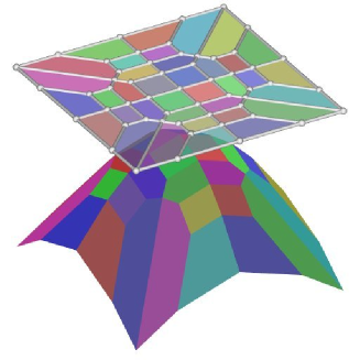
Figure 4.1: Computing the Voronoi diagram of a set of points using the lower envelope of a set of planes. The minimization diagram (appears above the envelope for clarity) of 36 planes, which represent distance functions to 36 point sites in a degenerate constellation, constitutes the Voronoi diagram of the points. The lower envelope, as well as the minimization diagram, are clipped to within an axis-aligned square.

Affine Voronoi diagrams is the class of all Voronoi diagrams whose sites have affine bisectors. The power diagram of a set of disks in the plane (defined below) is an affine Voronoi diagram and is a generalization of the standard Voronoi diagram of points. Interestingly, the class of affine Voronoi diagrams is identical to the class of power diagrams in the plane [bwy-cvd-06, §2.3.3]. Every abstract Voronoi diagram (Section 2.1) whose bisectors are lines has a corresponding power diagram that constitutes it. Therefore, having a robust implementation for computing power diagrams of sets of disks is, in some sense, a complete solution in this context.

Definition 4.1 (Planar power diagram).

The planar power distance is measured from a point $x\in{\mathbb{R}}\rule{0.85358pt}{0.0pt}^{2}$ in the plane to a disk $d$ with center $c$ and positive radius $r$, and is defined to be: $\rho(x,d)=(x-c)^{2}-r^{2}$. The power diagram of a set $D$ of disks in the plane is defined to be the nearest-site Voronoi diagram induced by the power distance.

Using a simple observation, one can construct the lower envelope of a set of planes instead of constructing the lower envelope of the paraboloids that represent the power distance functions from the disk sites. We transform each paraboloid of the form $f_{i}(x)=x^{2}-2xc+c^{2}-r^{2}$ to the plane $\pi_{i}:-2xc+c^{2}-r^{2}$. In other words, for each point $x\in{\mathbb{R}}\rule{0.85358pt}{0.0pt}^{2}$ and a site we remove the $x^{2}$ factor from the power distance. Notice that each distance function is decreased by the same amount for a specific point $x$, and thus, the topological structure of the lower envelopes of the original paraboloids and the new linear functions is identical. See Figure 4.1 for an illustration.

The Envelope_3 package of Cgal contains a traits class for constructing the lower or upper envelope of a set of planes and half-planes in ${\mathbb{R}}\rule{0.85358pt}{0.0pt}^{3}$, named CGAL::Env_plane_traits_3. However, as it might be expected, the implementation of this traits class is more complicated than is needed when considering the computation of power diagrams only (and not general envelopes). The reason is that the Env_plane_traits_3 traits class handles cases that cannot occur during the computation of power diagrams, i. e., the planes that represent power distance functions are always full planes and are never vertical.

We implemented an easy-to-use traits class for the computation of standard Voronoi diagrams of points and power diagrams of disks using our framework. The traits class is named CGAL::Power_diagram_traits_2 and is a model of the EnvelopeVoronoiTraits_2 concept (see Section 3.3). The implementation of the traits class is much simpler than the Envelope_3 package’s traits class, and provides a better interface for computing Voronoi diagrams — the user of the traits class does not need to construct any plane. A traits class modeling the EnvelopeVoronoiTraits_2 does not have to actually construct the distance functions from the sites; see Chapter 3. The Power_diagram_traits_2 traits class does not construct the three-dimensional planes, but directly implements all the required predicates and operations.

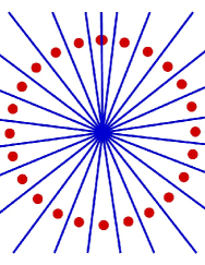
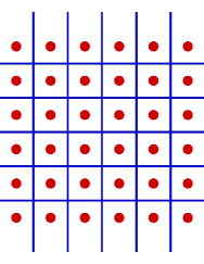
Figure 4.2: Voronoi diagrams of various point-sets computed with our framework and our traits class for computing power diagrams in the plane. 4.2 The Voronoi diagram of points ordered exactly on a circle. The Voronoi diagram has a single vertex. 4.2 The Voronoi diagram of points ordered on a grid. 4.2 The Voronoi diagram of points ordered on a cross. 4.2 The Voronoi diagram of points creating the letters of Cgal and VD (an abbreviation for Voronoi Diagrams).

Our traits class inherits from the CGAL::Arr_linear_traits_2 traits class [cgal:wfzh-a2-08] that models the ArrangementTraits_2 concept and supports arrangements induced by linear objects, which may be bounded (segments) or unbounded (rays and lines). The traits class is parameterized by a geometric kernel class [fgkss-dccga-00, hhkps-aegk-07]. The choice of the geometric kernel, which consists of types of constant size non-modifiable geometric primitive objects (e. g., points, lines, triangles, circles, etc.), and determines the number-type used and the implementations of all geometric operations on kernel objects. In this context, the geometric kernel determines, for example, the type representing the bisector curves (lines) and the number-type. The geometric kernel is passed as the underlying kernel for the Arr_linear_traits_2 base class.

The Power_diagram_traits_2 class requires the underlying number-type to only support exact rational arithmetic; as opposed to number types required in the following Sections 4.1.2 and 4.1.3. Namely, the number type should support the arithmetic operations $+$, $-$, $*$, and $/$ with unlimited precision over the rationals. An example for such number type is the rational number type CGAL::Gmpq based on Gmp— Gnu’s Multi Precision library gmp-link.

Disk sites (objects of type Site_2) are represented as unoriented circles in the two-dimensional Euclidean plane by the kernel type Kernel::Circle_2. In order to stay in the rational domain and apply only fast rational arithmetic operations, two restrictions on the disk sites must be enforced: the coordinates of their centers have to be rational, and the squares of their radii have to also be rational.

Although the new traits class provides a simpler implementation and a more convenient interface, it does not provide a significant increase in performance in comparison with the Env_plane_traits_3 traits class. The reason is that the main performance hit during the execution of the algorithm is caused, in fact, by the exact and expensive geometric operations and predicates that are provided by the kernel. Section 4.3 provides details on optimizations, which improve the computation time significantly. Most of the optimizations there concentrate on minimizing the number of calls to geometric operations and predicates.

Two-Site Triangle-Area Voronoi Diagram

Planar two-point distance functions are defined from a point $x$ in the plane to a pair of point site $\{p,q\}$. Among the known distance functions are (i) the sum of distances, which is defined by $\rho(x,\{p,q\})=d(x,p)+d(x,q)$ where $d$ is the Euclidean distance, (ii) the product of distances which is defined by $\rho(x,\{p,q\})=d(x,p)\cdot d(x,q)$, (iii) the triangle area distance function defined by the area of $\triangle xpq$, (iv) the triangle perimeter distance function defined by the perimeter of $\triangle xpq$, and (v) the difference of distances defined by $\rho(x,\{p,q\})=|d(x,p)-d(x,q)|$. The combinatorial complexity of the diagrams and the time complexity of the known algorithms for computing various two-point site Voronoi diagrams varies [bdd-psvd-02].

We describe in this section the implementation of a traits class named, Triangle_area_distance_traits_2 that enables the computation of the Voronoi diagram of points as induced by the triangle area distance function. The traits class uses rational arithmetic only and handles degenerate input.

The triangle distance function between a point $(x,y)$ in the plane and a pair of points $(p_{x},p_{y})$ and $(q_{x},q_{y})$ is defined to be the area of the triangle formed by these three points, namely,

$$\frac{1}{2}abs\left(\left|\begin{array}[]{ccc}x&y&1\\ p_{x}&p_{y}&1\\ q_{x}&q_{y}&1\end{array}\right|\right)\;.$$

The combinatorial complexity of the nearest-site Voronoi diagram of $n$ points in general position as induced by the triangle distance function is $\Theta(n^{4})$, and $\Theta(n^{2})$ for the farthest-site Voronoi diagram.

Triangle_area_distance_traits_2 is a model of the EnvelopeVoronoiTraits_2 concept. Similar to the Power_diagram_traits_2 traits class, our traits class inherits from the CGAL::Arr_linear_traits_2 traits class, which models ArrangementTraits_2 concept. The class is parameterized by a geometric kernel class whose number type is required to support exact rational arithmetic for achieving a robust implementation. The geometric kernel is passed to the Arr_linear_traits_2 base class as a template parameter.

The Voronoi sites (of Site_2 type) of our diagram are pairs of points. The user is accountable for providing all pairs of points as part of the input. The distance from a rational point in the plane to a pair of rational points is rational (due to the rational nature of the distance function). The Compare_distance_at_point_2 functor compares the two rational distances of a point in the plane to two 2-point sites.

The bisector of two sites consists of two rational lines. Let $S_{1}$ and $L_{1}$ be the segment connecting the two points of one site and its supporting line, respectively, and let $S_{2}$ and $L_{2}$ be the segment connecting the two points of another site and its supporting line, respectively. The intersection of $L_{1}$ and $L_{2}$ is the intersection of the two bisector lines. If $L_{1}$ and $L_{2}$ are parallel, then the bisector consists of two parallel lines that become the same line if $S_{1}$ and $S_{2}$ are of the same length. If $S_{1}$ and $S_{2}$ are collinear then the bisector is either one line, or, in case that $S_{1}$ and $S_{2}$ are of the same length, does not exist. We construct the two lines in the Construct_bisector_2 functor implementation. We have to perform an additional operation before outputting the two lines. The Envelope_3 package code does not tolerate bisectors whose $x$-monotone parts intersect in their interior. Before outputting the bisector we have to intersect the two lines and transform them into 4 interior-disjoint rays.

The last functor that is required by the EnvelopeVoronoiTraits_2 is the Compare_distance_above_2 functor. The bisector lines partition the plane into a maximum of 4 regions. If one of the points of a Voronoi site is inside a specific region, then the region is dominated by the Voronoi site of the point. When crossing a bisector we move from a region that is dominated by one site to a region that is dominated by the other site (except for the case where all four points are collinear). We compute the number of curves we need to cross to get from one of the points of the first site and from the region above the input curve to the upper-most face. (If we have a vertical line then we take the left one.) If both numbers are even or odd together we return that the region above the input curve is dominated by the first site. If one is odd and the other is even then the region is dominated by the second site.

4.1.2 Voronoi Diagrams with Higher-Degree Algebraic Bisectors

This section describes diagrams where exact rational arithmetic only is insufficient for computing the diagrams in an exact and robust manner. The presented diagrams are curved Voronoi diagrams [bwy-cvd-06] requiring a higher-degree algebraic machinery.

Möbius Diagrams

Definition 4.2 (Möbius diagram).

Let $w$ be a Möbius site defined by a triple $(p,\lambda,\mu)$ where $p\in{\mathbb{R}}\rule{0.85358pt}{0.0pt}^{2}$ and $\lambda,\mu\in{\mathbb{R}}\rule{0.85358pt}{0.0pt}$. The Möbius diagram of a set $\mathcal{W}=\{w_{1},\ldots,w_{n}\}$ of Möbius sites is the Voronoi diagram induced by the following distance function: $\rho(x,w_{i})=\lambda_{i}(x-p_{i})^{2}-\mu_{i}$

The Möbius diagram is a generalization of the power diagram of disks (Section 4.1.1) and of the multiplicatively-weighted Voronoi diagram. When all $\lambda_{i}$ are equal, the Möbius diagram becomes the power diagram of the set of disks centered at $p_{i}$ with radii $\sqrt{\frac{\mu_{i}}{\lambda_{i}}}$. When $\mu_{i}=0$ for all $i$, the Möbius diagram becomes the multiplicatively-weighted Voronoi diagram with $p_{i}$ as the points and $\sqrt{\lambda_{i}}$ as the weights.

The bisector of two Möbius sites is either a circle or a line (in case of equal $\lambda$ parameters). Moreover, every abstract Voronoi diagram whose bisectors are circles or lines has a corresponding Möbius diagram that constitutes it [bwy-cvd-06, §2.4.1] (similar to the relation of power diagrams and affine Voronoi diagrams).

Cgal contains a traits class for the arrangement package that supports arrangements of circular and linear bounded segments, named Arr_circle_segment_traits_2. The efficient implementation of the traits class, which supports these curves, is attained by the observation that the coordinates of all intersection points between the curves are of algebraic degree 2 only, and, therefore, can be represented with square-root extension numbers (which are an extension to the rational field).

We have created a model class for the EnvelopeVoronoiTraits_2 concept named CGAL::Mobius_diagram_traits_2, which supports the construction of Möbius diagram using our framework. The traits class supports rational Möbius sites (with rational $p$, $\lambda$, and $\mu$). The CGAL::Mobius_diagram_traits_2 class is based on an extension we have implemented for the Arr_circle_segment_traits_2, named Arr_circle_linear_traits_2, which supports, in addition, unbounded linear curves (lines and rays).

The fact that Arr_circle_linear_traits_2 harnesses efficient square-root extension arithmetic does not immediately imply that an implementation for the Möbius diagram that uses only square-root extension arithmetic (and not higher-degree algebraic numbers) is easily obtainable. Performing operations with square-root extension numbers is limited, since square-root extension numbers form an algebraic field only if they are extended by the same root. (Rational numbers are considered to be present in all extension fields.) This means that arithmetic operations on two square-root extension numbers can be easily performed, while staying in the same algebraic-degree arithmetic, only if they have the same extension.

We compute the distance from a point, which is of type Arr_circle_linear_traits_2::Point_2, to a Möbius site using square-root extension arithmetic. The $x$ and $y$ coordinates of a point of the Arr_circle_linear_traits_2 traits class are either both rational, one is rational and the other is a square-root extension number, or both are square-root extension numbers with the same extension. Therefore, we can perform all needed arithmetic operations for computing the distance by using square-root extension arithmetic.

Another non-trivial functor is the Construct_point_on_x_monotone_2 functor. In order to construct a point on an edge, assuming that the edge is not vertical, we construct isolating rational intervals for both of its endpoints. We use both intervals to get a rational $c$ between the endpoints and construct the vertical line $y=c$. The resulting point is the intersection point between this vertical line and the original edge. We perform similar operations in the cases of a vertical curve and an unbounded curve.

Anisotropic Voronoi Diagrams

Definition 4.3 (Anisotropic Voronoi diagram).

Let $s$ be an anisotropic site defined by the triple $(p_{i},M_{i},\pi_{i})$ where $p\in{\mathbb{R}}\rule{0.85358pt}{0.0pt}^{2}$, $M\in{\mathbb{R}}\rule{0.85358pt}{0.0pt}^{2\times 2}$ is a symmetric positive definite matrix, and $\pi\in{\mathbb{R}}\rule{0.85358pt}{0.0pt}$. The Anisotropic Voronoi diagram of a set $\mathcal{S}=\{s_{1},\ldots,s_{n}\}$ of anisotropic sites is the Voronoi diagram induced by the following distance function:

$$\rho(x,s_{i})=(x-p_{i})^{t}M_{i}(x-p_{i})-\pi_{i}$$

Anisotropic Voronoi diagrams are a natural generalization of Möbius diagrams (take the matrix $M$ to be the scalar $\lambda$ from Definition 4.2 times the identity matrix). Anisotropic Voronoi diagrams have various applications, e. g., guaranteeing the quality of meshes [ls-avdgqa-03].

The bisector of two Anisotropic sites is a full planar quadratic curve (i. e., a circle, an ellipse, a parabola, a hyperbola, or a degenerate version of one of the previous). Again, every abstract Voronoi diagram whose bisectors are full quadratic curves has a corresponding anisotropic diagram that constitutes it [bwy-cvd-06, §2.4.2].

We have created the Anistropic_voronoi_traits_2 traits class that enables the computation of anisotropic Voronoi diagrams using our framework. The traits class is based on a new traits class for the arrangement package that enables the construction of arrangements of algebraic plane curves [acs-be-cckva-08, ek-eeaaac-08]. The remaining required functors are a functor for constructing the bisector of two anisotropic sites and functors to answer proximity queries.

All required proximity predicates are similarly implemented as follows: we construct a point $p$ inside the region in question (rational points get a higher priority). Then, we compare the distances from $p$ to the two anisotropic sites and decide which of the sites is closer.

Deciding which of the sites is closer is a non-trivial task as we try to expedite the computation that involves expensive algebraic arithmetic. We use several techniques to optimize the computation. First, we try to construct an exact rational point (as opposed to a point of a higher algebraic degree). In most cases this is possible (but not in all, e. g., it is not possible to construct a rational point inside a singleton that consists of a non-rational point). Points with rational coordinates induce a rational distance, the computation of which is easy and fast. Second, if we are forced to construct a non-rational point, we first try to use rational interval arithmetic to decide the predicate [bbp-iaedf-01]. Each point represented by the algebraic plane curves traits class has a rational bounding-box with which we try and deduce a correct answer. Only if we can not use rational arithmetic to decide the predicate correctly, we resort to more expensive algebraic computations based on the Core library [klpy-clrngc-99]core-link.

4.1.3 Voronoi Diagrams with Semi-Algebraic Bisectors

In this section we describe the implementation of two important Voronoi diagrams, the Apollonius diagram (or additively-weighted Voronoi diagram) and the Voronoi diagram of linear objects. The bisectors of the two diagrams are semi-algebraic, i. e., composed of portions of algebraic curves. The implementation of both diagrams is based on the algebraic plane curve traits class mentioned in the previous section. We concentrate on the additional problems introduced by the computation of Voronoi diagrams with semi-algebraic bisectors. Those problems include, among others, non-rational distance functions and complicated boundary conditions.

Apollonius Voronoi Diagrams

The Apollonius diagram, also known as the additively-weighted Voronoi diagram, has applications in many fields [obsc-stcavd-00, ada-msawvd-07]. It is often used as a replacement for the Voronoi diagram of circles in the plane. (See Chapter 6 for a concrete application of the Apollonius diagram — computing a minimum-width annulus of a set of disks.)

Definition 4.4 (Apollonius diagram).

Given a set $D=\{d_{1},\ldots,d_{n}\}$ of disks with respective centers $p_{i}$ and radii $r_{i}$, the Apollonius diagram of the set is the diagram induced by the following distance function: $\rho(x,d_{i})=||x-p_{i}||-r_{i}$

Given two disks in the plane, their Apollonius bisector is either (i) one branch of a hyperbola, which “bends” toward the disk with the smaller radius, (ii) a line, which is the bisector of the centers of the disks, in case of equal radii, or (iii) the empty set in the case where one disk contains the other (there is no bisector as one site dominates the whole plane). In the case that the bisector is a branch of a hyperbola, the transverse axis of the hyperbola is the line passing through the centers of the disks.

The traits class Apollonius_traits_2 enables the construction of Apollonius diagrams using our framework, and handles all degenerate cases (including all types of bisectors). The implementation of this traits class is similar to the implementation of the traits class for the anisotropic diagram (see Section 4.1.2 above). There are two main differences in the implementation of the Apollonius_traits_2 class. The first is the construction of the bisector of two Apollonius sites, which is not a simple full algebraic curve. The second is that the distance function between a point in the plane and an Apollonius site is not “rational,” meaning that the distance is not necessarily rational even if the given point is.

The construction of a bisector amounts to the following task. Given the full algebraic hyperbolic curve, pick the correct branch and return it. We efficiently implement the functor for constructing the bisector by exploiting the Make_x_monotone_2 functor of the algebraic curves traits class. The Make_x_monotone_2 of the traits class not only splits the hyperbola into two/four different $x$-monotone curves, but also fortunately returns them in a lexicographic order. By examining the coordinates of the centers of the disks and their radii, we can determine which of the two branches is the bisector. For example, in the case of a vertical asymptote, we pick the correct branch by comparing the $x$-coordinates of the centers of the disks; the correct branch is the one on the same side as the disk of the smaller radius. Notice, that if one Apollonius site contains another site then there is no bisector between them and the site with the larger radius dominates the entire plane.

The distance function from a point in the plane to an Apollonius site is not rational. Even if a rational point is given, the resulting distance is not necessarily rational. Still, comparing the distances of a rational point to two Apollonius sites is faster than of a non-rational point. A rational point results in a distance value of algebraic degree 2 where a general point of the traits class may result in a number of algebraic degree up to 8. Again, we use the Core library for comparing numbers of high algebraic-degree in an exact manner.

Voronoi Diagrams of Linear Objects

The Euclidean Voronoi diagram of segments in the plane is probably the most frequently used Voronoi diagram after the Voronoi diagram of points. We present an exact implementation for a traits class for the computation of the Voronoi diagram of a set of interior-disjoint linear geometric objects (lines, rays, and line segments) and points. Figure 4.3 shows diverse cases of Voronoi diagrams of linear objects computed with our traits class. Other exact implementations for the Voronoi diagram of segments include the one provided by Cgal [k-reisvd-04, cgal:k-sdg2-08] and the divide-and-conquer algorithm by Aichholzer et al. [aaahjp-dcvdr-09a], which uses Cgal predicates as basic building-blocks. Both implementations do not support ray sites and line sites. The algorithm by Aichholzer et al. uses a circle to bound the Voronoi edge-graph. A bounding circle cannot contain unbounded linear entities, such as lines and rays. Our implementation here is aimed at demonstrating the generality of our framework.

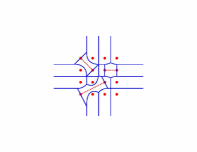
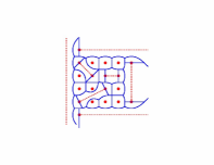
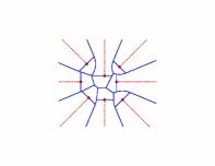
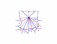
Figure 4.3: Voronoi diagrams of various sets of linear objects as induced by the Euclidean metric computed with our framework. The sites are illustrated with dashed curves. 4.3 The Voronoi diagram of 4$\times$4 grid with three line segments connecting 6 grid points. 4.3 The same set of sites as in 4.3 with a line, a segment, and two rays around the grid points. 4.3 The Voronoi diagrams of 8 rays in the plane. 4.3 The Voronoi diagram of 8 segments and 7 isolated points. All segments intersect at one point, which is one of their endpoints.

As mentioned before, the bisectors of two points or two lines in the plane are composed of linear curves. The bisector of a point and a line is a parabola. As a result, the bisector of two sites in the plane is composed of linear objects (segments, rays, and lines) and parabolic arcs. The bisector of two segments can be composed of up to 7 arcs [y-avdssc-87]. It should be noted that even computing just the linear bisectors of the diagram is not a trivial task. Indeed, the bisector of two lines is two perpendicular lines, but those lines do not necessarily possess rational coefficients. We support segments with intersecting vertices, which can induce two-dimensional bisectors as the region dominated by the joint vertex can be two-dimensional.

The traits class Linear_objects_Voronoi_traits_2 uses the following technique to deal with the two-dimensional bisectors and the relative complex structure of the bisector curves. The traits class treats each segment as a set of 3 different Voronoi sites: the two vertices of the segment and the open set that is the interior of the segment. The handling of all predicates, specifically predicates related to bisector construction, is made much simpler at the cost of an enlarged set of sites. The splitting of a site into several sites is implemented in the Make_xy_monotone_3 functor of the EnvelopeTraits_3 concept (this functor is not part of the EnvelopeVoronoiTraits_2 concept). The class Linear_objects_Voronoi_traits_2 models the EnvelopeTraits_3 concept rather than the EnvelopeVoronoiTraits_2 concept.

The interior of a segment behaves like a full straight line inside the region between the two perpendicular lines at its vertices. Moreover, it has no effect on any other point outside that region as the vertices of the segment dominate the rest of the Euclidean plane. The domain of the distance function to the interior of the segment is, therefore, defined to be the aforementioned region. The domain of a ray is the half-plane that contains it and bounded by the perpendicular line at its source. The domain of a distance function to a point site and a line site remains the whole plane. We implement this by providing the functor Construct_projected_boundary_2 defined in the EnvelopeTraits_3 concept.

After the splitting we only need to consider three types of bisectors, namely, the bisector between two points, the bisector between two lines (where a line can also relate to the interior of a segment or a ray) that is a two-line bisector, and the bisector between a point and a line, which is a full parabola.

Comparing the distances of a point in the plane to two points or two linear objects is trivial: we just compare the “regular” squared distance from that point to the sites. When comparing the distances to a point and to a linear object we have to be more careful, as the interiors of segments and rays are not closed sets. We compare the squared distances to the point and to the linear object. If an “equal” result is the outcome of considering an endpoint of the linear object, we decide that the point site is closer, as the endpoint of a linear object (a segment or a ray) is not contained in its interior.

The final problem we have to face is that the bisector of two lines in the plane is two lines that do not have rational coefficients in the general case. We observe that these two lines constitutes a degenerate hyperbola with rational coefficients. We use the algebraic traits class to construct the degenerate hyperbola that represents the bisector of the two input lines.

4.2 Spherical Voronoi Diagrams

The computation of Voronoi diagrams makes use of two main operations supported by the Arrangement_on_surface_2 package: (i) sweep-based overlay operation, which is used to overlay two minimization diagrams, and (ii) zone computation-based insertion operation, which is used to insert bisector curves that partition cells of the refined arrangement; see Chapter 3.

The new Arrangement_on_surface_2 package extends the aforementioned operations, that is, the sweep-line and zone-computation, to support two-dimensional parametric surfaces. Thus, we utilize the Envelope_3 code to handle minimization diagrams that are embedded on two-dimensional parametric surfaces with little effort.

This section demonstrates how the ability of constructing arrangements on two-dimensional parametric orientable surfaces is exploited to compute Voronoi diagrams on the sphere We compute Voronoi diagrams, the bisectors of which are composed of geodesic arcs, namely, arcs of great circles which are created by intersecting the sphere with planes passing through the origin. Section 4.2.1 gives some details about the traits class we have created for the arrangement package that enables us to construct arrangements of geodesic arcs on the sphere using rational arithmetic only. Section 4.2.2 describes how we use the above traits class to create a traits class for our Voronoi framework for computing Voronoi diagrams embedded on the sphere, the bisectors of which are geodesic arcs — the Voronoi diagram of points on the sphere and the power diagram of circles on the sphere. The section focuses on the implementation details involved in the development of a Voronoi diagram embedded on a two dimensional parametric surface.

Further details on the requirements from a traits class that enables the computation of Voronoi diagrams on surfaces can be found in Section 3.3. Details on constructing arrangements on surfaces in general, and on constructing geodesic arrangements on the sphere in particular, can be found in [bfhmw-smtdas-07, fsh-eiaga-08] and in Efi Fogel’s Ph. D. thesis [f-mscaag-08].

4.2.1 Arrangements of Geodesic Arcs on the Sphere

Complying with the specifications in [bfhmw-smtdas-07], we use the following parameterization of the unit sphere: $\Phi=[-\pi+\alpha,\pi+\alpha]\times[-\frac{\pi}{2},\frac{\pi}{2}]$, $\phi_{S}(u,v)=(\cos u\cos v,\sin u\cos v,\sin v)$, where $\alpha$ must be substituted for a value, which yields rational $\cos\alpha$ and rational $\sin\alpha$ and defaults to $0$, when the class is instantiated (at compile time). The equator curve, for example, is given by $\gamma(t)=(\pi(2t-1)+\alpha,0)$, for $t\in[0,1]$. This parameterization induces two contraction points $p_{s}=(0,0,-1)=\phi_{S}(u,-\frac{\pi}{2})$ and $p_{n}=(0,0,1)=\phi_{S}(u,\frac{\pi}{2})$, referred to as the south and north poles, respectively, and an identification curve $\{\phi_{S}(\pi+\alpha,v)\,|\,-\frac{\pi}{2}\leq v\leq\frac{\pi}{2}\}$, as $\phi_{S}(-\pi+\alpha,v)=\phi_{S}(+\pi+\alpha,v)$ for all $v$ (which coincides with the opposite Prime (Greenwich) Meridian when $\alpha=0$). We developed the topology traits to support any type of curves embedded on the sphere parameterized as above, without compromising the performance of the operations gathered in the traits class. We concentrate on the details of the geometric traits class as it is most relevant in this section.

The geometry-traits class for geodesic arcs on the sphere is parameterized with a geometric kernel [hhkps-aegk-07]; see also Section 4.1.1. The implementation handles all degeneracies, and is exact as long as the underlying number type supports the arithmetic operations $+$, $-$, $*$, and $/$ only in unlimited precision over the rationals, such as the one provided by Gmp, the Gnu Multi-Precision bignum librarygmp-link, even though the embedding surface is a sphere. We are able to use high-performance kernel models instantiated with exact rational number-types for the implementation of this geometry-traits class, as exact rational arithmetic suffices to carry out all necessary algebraic operations.

The geometry-traits class defines the point type to be an unnormalized vector in ${\mathbb{R}}\rule{0.85358pt}{0.0pt}^{3}$, representing the place where the ray emanating from the origin in the relevant direction pierces the sphere. An arc of a great circle is represented by its two endpoints, and by the plane that contains the endpoint directions and goes through the origin. The orientation of the plane and the source and target points determine which one of the two arcs of the great circle is considered. This representation enables an exact, yet efficient, implementation of all geometric operations required by the geometry-traits concept using exact rational arithmetic, as normalizing directions and plane normals is completely avoided.

We describe in details two predicates: Compare $u$ and Compare $uv$; see [f-mscaag-08] for the

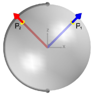
Figure 4.4: The implementation of the Compare-$u$ predicate in the traits class for geodesic arcs on the sphere

complete set of the concept requirements. The former compares two points $p_{1}$ and $p_{2}$ by their $u$-coordinates. The concept admits the assumption that the input points do not coincide with the contraction points and do not lie on the identification arc. Recall that points are in fact unnormalized vectors in ${\mathbb{R}}\rule{0.85358pt}{0.0pt}^{3}$. We project $p_{1}$ and $p_{2}$ onto the $xy$-plane to obtain two-dimensional unnormalized vectors $\hat{p_{1}}$ and $\hat{p_{2}}$, respectively. We compute the intersection between the identification arc and the $xy$-plane to obtain a third two-dimensional unnormalized vector $\hat{d}$. Finally, we test whether $\hat{d}$ is reached strictly before $\hat{p_{2}}$ is reached, while rotating counterclockwise starting at $\hat{p_{1}}$. This geometric operation is supported by every geometric kernel of Cgal. In the figure on the right $\hat{d}$ is reached strictly before $\hat{p_{2}}$ is reached. Therefore, the $u$-coordinate of $p_{1}$ is larger than the $u$-coordinate of $p_{2}$.

The predicate Compare $uv$ compares two points $p_{1}$ and $p_{2}$ lexicographically. It first applies Compare $u$ to compare the $u$-coordinates of the two points. If the $u$-coordinates are equal, it applies a predicate that compares the $v$-coordinates of two points with identical $u$-coordinates, referred to as Compare $v$. This predicate first compares the signs of the $z$-coordinates of the two unnormalized input vectors. If they are identical, it compares the squares of their normalized $z$-coordinates, essentially avoiding the square-root operation.

All the required geometric types and geometric operations listed in the geometric traits concept are implemented using rational arithmetic only. Degeneracies, such as overlapping arcs that occur during intersection computation, are properly handled. The end result is a robust, yet efficient, implementation.

4.2.2 Power Diagrams on the Sphere

The spherical Voronoi diagram and its generalization, the power diagram of circles on the sphere (both defined below) are composed of geodesic arcs. Both diagrams have applications similar to the applications of Voronoi diagrams of points and power diagrams in the plane. For example, determining whether a point is included in the union of circles on the sphere, and finding the boundary of the union of circles on the sphere [iim-vdlgia-85, s-lvds-02]. Both also have unique applications, for example, the properties of the spherical Voronoi diagram can be used to prove the the thirteen spheres theorem [a-tsnp-04].

Following are definition for the geodesic distance on the sphere (which is the analog of the Euclidean distance between two points in the plane) and the spherical Voronoi diagram (which is the analog of the Voronoi diagram of points in the plane).

Definition 4.5 (Geodesic distance).

Given two points $p,q\in{\mathbb{S}}\rule{0.85358pt}{0.0pt}^{2}$, the geodesic distance between them $\rho(p,q)$ is defined to be the shortest distance measured along a path on the surface of the sphere. The geodesic distance $\rho(p,q)$ is equal to the length of a geodesic arc that connects $p$ and $q$.

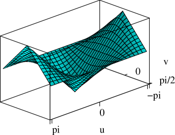
Figure 4.5: Geodesic distance function on the sphere.

Figure 4.5 to the right illustrates the distance function from $(0,0)\in[-\pi,\pi]\times[-\frac{\pi}{2},\frac{\pi}{2}]$ in the parameter space (defined in Section 4.2.1 above) to any other point in the parameter space. As expected from the topology of the surface, we get a function whose values are identified at the boundaries of the parameter space. Fortunately for us, we do not have to explicitly construct and handle these types of functions. We only have to correctly answer the predicates that are required by the algorithm. The central projection of the intersection of two such functions onto the sphere is a great circle, as the bisector of two points on the sphere as induced by the geodesic distance is a great circle.

Definition 4.6 (Spherical Voronoi diagram).

Let $P=\{p_{1},\ldots,p_{n}\}$ be a set of $n$ points in ${\mathbb{S}}\rule{0.85358pt}{0.0pt}^{2}$. The spherical Voronoi diagram of the set $P$ is the Voronoi diagram as induced by the geodesic distance function.

The bisector of two point sites on the sphere is a great circle that is the intersection of the sphere and the bisector plane of the points in ${\mathbb{R}}\rule{0.85358pt}{0.0pt}^{3}$, as imposed by the Euclidean metric [nlc-vds-02, obsc-stcavd-00]. The power diagram of circles on the sphere, also known as the Laguerre Voronoi diagram on the sphere, is also composed of arcs of great circles [s-lvds-02]; see Figures 4.6 and 4.6.

Given two circles on the sphere $c_{1}$ and $c_{2}$, let $\pi_{1}$ and $\pi_{2}$ be the planes containing $c_{1}$ and $c_{2}$, respectively. The bisector of $c_{1}$ and $c_{2}$ is the intersection of the sphere and the plane that contains the intersection line of $\pi_{1}$ and $\pi_{2}$ and the center of the sphere. If $\pi_{1}$ and $\pi_{2}$ are parallel planes, then the bisector is the intersection of the sphere and the plane that contains the center of the sphere and is parallel to both $\pi_{1}$ and $\pi_{2}$.

We believe that the following argument, similar to arguments in previous sections, is true; more details are supplied in Chapter LABEL:chap:conclusion.

Conjecture 4.7.

The class of all Voronoi diagrams with great circles as bisectors is identical to the class of power diagrams of circles on the sphere.

The Arr_geodesic_arc_on_sphere_traits_2 traits class for computing arrangements of geodesic arcs on the sphere provides predicates and operations needed for the computation of Voronoi diagrams on the sphere, the bisectors of which are great circles or piecewise curves composed of geodesic arcs. It is the basis of the Spherical_power_diagram_traits_2 class that enables the construction of power diagrams of sets of circles on the sphere using our framework. The traits class applies only rational arithmetic, and so, only Voronoi diagrams of circles defined by the intersection of rational planes with the sphere (and rational points on the sphere) are supported. This is not a very strong limitation as every input point can be approximated with a rational point up to any desired precision [cdr-rrmrg-92].

The Spherical_power_diagram_traits_2 is a model of the EnvelopeVoronoiTraits_2 concept and defines all required types and functors. It is parameterized by a geometric kernel of Cgal that is passed also to the Arr_geodesic_arc_on_sphere_traits_2 base class. The kernel should support exact rational number-types to carry all necessary operation in an exact manner. The traits class handles all degenerate situations efficiently.

A Site_2 in the Spherical_power_diagram_traits_2 is an object of type Kernel::Plane_3 — a 3D plane object of the geometric kernel. The plane represents the Voronoi site that is the circle intersection of the plane and the embedding sphere. Not all planes in three dimensions can represent a site in our traits class. Recall that we are constructing the arrangement on the sphere, so only planes whose distance from the origin is $\leq 1$ are used. The Construct_bisector_2 functor is responsible for constructing the bisector of two circle sites on the sphere. It intersects the two underlying planes of the Voronoi sites, and constructs the great circle that is defined by the plane containing the intersection line and the origin. In the case that both planes are parallel, we construct the great circle that is defined by the plane parallel to both planes and passing through the origin.

The functor Construct_point_on_x_monotone_2 constructs a point in the interior of a $u$-monotone curve. Every $u$-monotone arc has a source point and a target point. Recall that points are represented as unnormalized vectors in three-dimensions. If the geodesic arc is smaller than $\pi$, adding the source and target vectors results in an unnormalized vector that represents a point in the interior of the arc. If the geodesic arc is bigger than $\pi$ we construct the opposite vector. The case where the geodesic arc is equal to $\pi$, in which the source and target are antipodal, is handled by constructing an orthogonal vector to both the target vector and the normal of the plane. The resulting vector represents a point in the interior of the $u$-monotone arc.

The remaining functors are the proximity predicates Compare_distance_at_point_2 and Compare_distance_above_2. The former predicate is given two circle sites (defined by two planes) and a point on the sphere (defined by a vector) and is to decide which of the sites the point is “closer” to. The circle that is closer to the point is the one defined by the plane encountered first when shooting a ray in the direction of the point from the origin. The predicate intersects the underlying planes with the line passing through the origin and the input point. Then, it compares the distances of the intersection points to the origin. An intersection point could be in the same direction as the input point from the origin, or in the opposite direction. A site whose intersection point is in the opposite direction is considered farther from the input point than a site whose intersection point is in the same direction. If the intersection points of both circles are in the opposite direction, the opposite result is returned. If one of the planes is parallel to the vector that represents the input point then, if the intersection point of the other site is in the same direction, the other site is closer, otherwise the site with the underlying parallel plane is closer. If both planes are parallel to the vector of the point we have an equality.

The Compare_distance_above_2 is implemented by considering the geodesic arc itself and the planes that define the two sites. We observe the $u$ and $v$ coordinates of the normals to the planes and deduce an answer. This is similar to the implementation of the same functor in the power diagram of disks in the plane; see Section 4.1.1. The main difference is that on the sphere, circles with the same center but with different radii still have a bisector, whereas in the plane the disk with the larger radius dominates the whole plane. In other words, two sites always have a bisector. If the normals to the planes are in the same direction (circles having the same center) then the distance of the planes to the origin (radii of the circles) is also considered while deducing an answer.

Figure 4.6 shows some Voronoi diagrams on the sphere. Figures 4.6 and 4.6 are of specific interest as they constitute highly degenerate scenarios.

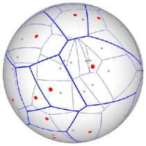
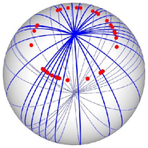
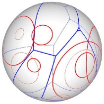
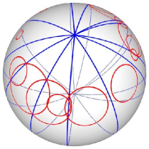
Figure 4.6: Voronoi diagrams on the sphere. Sites are drawn in red and Voronoi edges are drawn in blue. 4.6 The Voronoi diagram of 32 random points. 4.6 A highly degenerate case of Voronoi diagram of 30 point sites on the sphere. 4.6 The power diagram of 10 random circles. 4.6 A degenerate power diagram of 14 sites on the sphere.

4.3 Speeding-up the Computation

The main performance hit during the execution of our algorithm (and exact geometric algorithms in general) is caused while trying to exactly evaluate geometric predicates, i. e., using exact arithmetic operations. There is a conceptual efficiency scale of operations, ranging from the most efficient operations to the less efficient operations. The most efficient operations are the ones using machine-supported arithmetic, such as integers and floating-point numbers. Using exact rational-arithmetic is less efficient than the machine-supported arithmetic, but is still much faster than using exact higher-degree algebraic computation. As the algebraic degree goes up, the performance of operations goes down.

There are several optimizations that can be applied to a geometric algorithm. The first is trying to use the more efficient arithmetic according the scale described above. If the used arithmetic fails we go down the scale of efficiency and use a higher-precision or higher algebraic-degree arithmetic. Alternatively, one can try and use simpler (approximated) operations to the reduce the use of the exact and complicated operations (e. g., when performing an intersection test between two polylines, the intersection of their bounding boxes can be tested first). Another technique is to reduce the number of (redundant) geometric operations used. The technique of using a simpler approximated version of a predicate to alleviate the use of the more expensive operation is referred to as filtering. When the filtering exploits the specific geometry of the problem at hand it is referred to as geometric filtering. We describe below techniques we have applied to reduce the running time of our algorithm in the context of affine Voronoi diagrams; Section 4.1.1. We use fast geometric filters and apply specific techniques at a high level for (affine) Voronoi diagrams that reduce lower-level filter-failures.

Most implementations of traits classes for our framework are based on traits classes for the arrangement package. The first step in optimizing the code is to pick the most efficient traits class to handle the bisector curves of the specific diagram. The Arr_linear_traits_2 class is parameterized with a kernel object, the choice of which has a drastic effect on the performance of our code.

Cgal provides basic geometric kernels with built-in filtering mechanisms. The CGAL::Lazy_kernel class is an efficient geometric kernel of Cgal [fp-gleseg-06], which supplies lazy construction and evaluation of the geometric predicates and operations that delay the exact geometric computations at run-time. Every geometric object of the CGAL::Lazy_kernel class holds two other instances of different classes; one instance is approximated using machine floating-point interval-arithmetic, and the other instance is exact using rational arithmetic. The kernel tries to use the fast machine arithmetic, and only if it fails, it performs the required operation using the exact version of the object. Every geometric object that was created using kernel operations keeps the tree of operations that created it. This way, when an approximated operation fails, the tree of operations can be retrieved and the operations are performed all over again using the exact version. However, if an operation does not fail, no costly operation is performed (a lazy behavior). This filtering mechanism is applied at the geometric level, which proved to be more efficient than the regular interval-arithmetic filtering mechanisms that are applied at the arithmetic (number-type) level. We use the CGAL::Lazy_kernel as the base for our traits class in the case of Voronoi diagrams with linear bisectors. A future work is to implement a traits class for the Möbius diagram using the CGAL::Circular_kernel_2 with other geometric filtering optimizations [ptt-gfpca-06]; see Chapter LABEL:chap:conclusion.

The aforementioned geometric kernels and traits classes for the arrangement package provide a very general approach for accelerating geometric computations. However, the filtering techniques applied at this low level are not aware of certain properties of the specific problem at hand, which can be exploited to improve performance. Specifically, the lower envelope algorithm applies some geometric predicates that incur geometric filter-failures due to the combinatorial structure of Voronoi diagrams. With a simple observation, we can avoid those filter-failures during the execution of the divide-and-conquer algorithm, increasing the efficiency of our code.

Observation 4.8.

Given three Voronoi sites and their pairwise bisectors, if two of the bisectors intersect then the third bisector passes through their intersection point(s).

Indeed, denoting the sites by $o_{1}$, $o_{2}$, and $o_{3}$, then at every intersection point $x$ of any two of the three corresponding bisectors, we have $\rho(x,o_{1})=\rho(x,o_{2})=\rho(x,o_{3})$.

The merge step of the divide-and-conquer of algorithm (see Section 3.1) consists of determining the structure of the Voronoi diagram over each face $f$ of the overlay of ${\rm Vor}_{\rho}(S_{1})$ and ${\rm Vor}_{\rho}(S_{2})$. The face $f$ has a fixed nearest site $s_{1}$ from $S_{1}$ and a fixed nearest site $s_{2}$ from $S_{2}$. We partition $f$ into subfaces consisting of points nearer to $s_{1}$ and subfaces consisting of points nearer to $s_{2}$ by inserting their bisector into the arrangement.

If $f$ is split into at least two regions, then the bisector of $s_{1}$ and $s_{2}$ generally intersects some edges of $f$. Let us assume, without loss of generality, that the bisector intersects an edge $e$ that originally belonged to ${\rm Vor}_{\rho}(S_{1})$. The edge $e$ is part of the bisector between $s_{1}\in S_{1}$ and another site $t\in S_{1}$. Assuming general position, when examining the neighboring face $f^{\prime}$ of $f$ on the other side of $e$, the two fixed nearest sites are $t\in S_{1}$ and $s_{2}\in S_{2}$. According to Observation 4.8 the bisector of $t$ and $s_{2}$ will pass through the intersection points of the bisector of $s_{1}$ and $s_{2}$, and $e$.

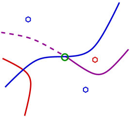
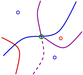
Figure 4.7: Three-bisectors optimization. During the merge step of the blue and red Voronoi diagrams each face is split by the bisector of the two nearest sites of both diagrams. 4.7 The bisector of the right blue site and the red site splits the right face. 4.7 The bisector of the left blue site and the red site splits the left face. Notice that the bisector passes through the intersection point of the former bisector and the boundary of the right face (the intersection point is circled in green).

Table 4.1: Effect of the three-bisector and simplified zone optimizations on random points. Time is measured in seconds. FF — the number of filter-failures that occurred during the computation, V — the number of vertices of the diagram, E — the number of edges of the diagram, F — the number of faces of the diagram, 3-Bis. — the three-bisector optimization, S-Z — the simplified zone optimization.

Input	Diagram Size			No opt.		3-Bis. opt.		3-Bis. + S-Z
	V	E	F	Time	FF	Time	FF	Time	FF
rnd_1000	1979	2978	1000	5.52	75105	3.58	11408	2.72	599
rnd_2000	3983	5982	2000	12.57	168411	8.30	25099	6.58	1285
rnd_4000	7979	11978	4000	28.54	370848	19.66	58098	15.41	2807

Each feature of the overlay is extended with the nearest Voronoi sites to it. When inserting a bisector into the overlay and creating a new vertex at the intersection point, we update the information of the new vertex. When inserting another bisector to the overlay and trying to decide if a point is on the bisector curve, we first check this information instead of using a geometric predicate, which is redundant and would have caused a filter to fail. We call this optimization the three-bisectors optimization; see Figure 4.7 for an illustration.

A bisector curve is inserted into the underlying arrangement using a zone-construction algorithm. The zone-construction algorithm of the arrangement package is most general and can handle any input, including a face that contains inner-holes, isolated vertices, or “antennas” [wfzh-aptaca-07]. In the case of a Voronoi diagram with affine bisectors we always insert the bisector curve into a convex face (with no inner holes). We use a simplified version of the zone algorithm, which gives us additional performance improvement.

The simple version works in the case of inserting a curve (line) into a bounded convex face (that is composed of linear segments). First, we try to detect if one of the vertices of the faces was created by inserting a bisector (a vertex that will invoke the three-bisector optimizations). This avoids the costly operations performed by the regular zone algorithm for finding the vertex by traversing the edges of the face. After we have found a maximum of two intersection points we stop, as this is the maximum number of intersections. Additionally, we do not check intersections with inner holes and do not consider other degenerate situations. For the other cases, i. e., inserting a line into an unbounded face or a zone-insertion that admits an overlap, we use the standard zone algorithm supplied by the arrangement package. Table 4.1 shows the improvements in running time achieved by our optimizations.

Chapter 5 Discussion: Advantages and Limitations

Our framework consists of several fundamental concepts: (i) robust computation through the adherence to the exact computation paradigm, utilizing components from Cgal, (ii) using randomization on the input to the divide-and-conquer construction algorithm, yielding an efficient algorithm, and (iii) the representation of Voronoi diagrams as arrangements, Cgal’s arrangements to be precise.

Following is a comprehensive discussion on both the advantages and the limitations of our framework. The advantages are discussed in Section 5.1 and the limitations are discussed in Section 5.2.

5.1 Advantages

The major strength of our approach is its completeness, robustness, and generality, that is, the ability to handle degenerate input, the agility to produce exact results, and the capability to construct diverse types of Voronoi diagrams with a relatively small effort. The code is designed to successfully handle degenerate input, while exploiting the synergy between generic programming and exact geometric computing, and the divide-and-conquer framework to construct Voronoi diagrams.

Generality

A prime advantage of our framework is the ability to compute new types of Voronoi diagrams with relative ease. The diagrams are represented as arrangements of Cgal, and the implementation of a new type of diagrams is based on a traits class for the arrangement package, which supplies the handling of bisector curves of the sites. A Voronoi diagram whose bisectors can be represented with an existing traits class for the arrangement package can be easily developed. Existing traits classes support bounded and unbounded linear curves (line segments, rays, and lines), circles and linear segments, conic arcs, Bézier curves, and algebraic curves of arbitrary degree.

The framework supports a vast variety of Voronoi diagrams with different properties. The entire collection of supported Voronoi diagrams cannot be supported by most other frameworks. Existing frameworks for computing Voronoi diagrams usually support a specific family of Voronoi diagrams, e. g., planar Voronoi diagrams of points under the $L_{p}$ metric, planar Voronoi diagrams of general sites under the Euclidean metric etc. Using an envelope-construction based algorithm allows our framework to support two-dimensional diagrams with almost no restrictions; we can implement linear Voronoi diagrams as well as Voronoi diagrams with quadratic complexity, and Voronoi diagrams with two-dimensional bisectors. The diagrams do not have to conform with the abstract Voronoi diagrams definition, for example anisotropic diagrams: we construct such diagrams whereas the theoretical requirements for an abstract Voronoi diagram include that all bisectors will divide the plane into two unbounded regions. As mentioned before, we can also compute Voronoi diagrams on two-dimensional orientable parametric surfaces. Existing topology-traits classes in the arrangement package include a topology-traits class for the plane, the sphere, elliptic quadrics, and ring Dupin cyclides that generalize tori.

More information on realizations of the framework can be found in Chapter 4.

Theoretical Optimality

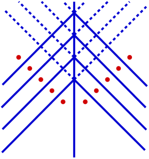
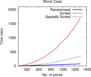
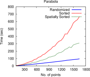
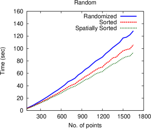
Figure 5.1: Effect of the random partitioning of Voronoi sites. The figure shows the running time in seconds as a function of the number of sites in various cases of the standard Voronoi diagram (point sites with $L_{2}$ metric) using different partitioning strategies. 5.1 A worst-case example of 10 point sites in the case of the standard Voronoi diagram. The dashed segments are segments that exist in the overlay (if we use the “Sorted” partition strategy) but will not be present in the final diagram. 5.1 The running time graph in the worst-case constellation where the point sites are arranged as in 5.1. 5.1 The running time graph in the case where the point sites are on a single parabola. 5.1 The running time graph in the case of random point sites inside a square.

The random partitioning of the Voronoi sites into two sets in the divide step of the algorithm yields a near-optimal expected running time in the size of the output diagram (Section 3.4). This optimality result is general, and true for every type of diagrams supported by the framework.

Figure 5.1 demonstrates the effect of randomly partitioning the sites on the standard Voronoi diagram of points with diverse sets of inputs. We apply the following three different partitioning strategies: (i) the partitioning based on lexicographic sort (Sorted) — the first set comprises the smaller $\lceil n/2\rceil$ points and the second set of points comprises the larger $\lfloor n/2\rfloor$ points, (ii) a partitioning based on CGAL::spatial_sort function (Spatial Sorted), and (iii) a randomized partitioning (Randomized). In all cases, if we randomly partition the sites, we get a nearly-linear running time in the number of sites. In the case of a random point-set (Figure 5.1) we get a slightly larger, though still nearly-linear, running time.

Figure 5.1 uses the following set of inputs. Each input set of $n$ points is defined to be $\{(i,i)\}_{i=1}^{n/2}\cup\{(-i,i)\}_{i=1}^{n/2}$. If we partition the set into two subsets, to the left and to the right of the $y$-axis (the “Sorted” partitioning strategy), then the overlay of the two Voronoi diagrams has $\Theta(n^{2})$ complexity; see Figure 5.1 for an illustration. Hence the algorithm runs in $\Omega(n^{2})$ time, whereas the complexity of the final diagram is only $\Theta(n)$.

Handling Degeneracies

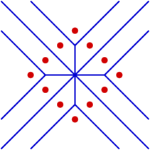
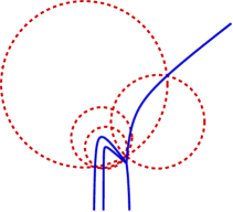
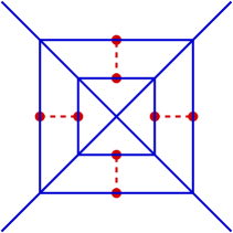
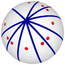
Figure 5.2: Degenerate Voronoi diagrams computed with our software. 5.2 A degenerate standard Voronoi diagram. 5.2 A degenerate additively-weighted Voronoi (Apollonius) diagram. 5.2 A degenerate Voronoi diagram of segments. 5.2 A degenerate spherical Voronoi diagram. The sites in 5.2 and 5.2 are illustrated with dashed curves.

Implementing robust geometric algorithms is known to be a hard task [kmpsy-cerpg-08]. Inherent problems in designing geometric algorithms are the coping with the limited precision of machine-supported arithmetic and the handling of complicated boundary conditions that arise in various degenerate situations (see Section 2.3). Our framework, like the Arrangement_on_surface_2 package of Cgal, handles all degenerate situations while computing Voronoi diagrams, as long as the supplied traits class handles a small number of degenerate cases. For example, the traits class should detect if two $x$-monotone curves overlap when trying to intersect them. All implemented traits classes described in Chapter 4 handle all degenerate situations. Figure 5.2 depicts various degenerate situations that are properly handled by our framework and the traits classes.

Farthest-site Voronoi diagrams

A useful meta-type of Voronoi diagrams is the farthest-site Voronoi diagram. A farthest Voronoi diagram can be formalized as a nearest-site Voronoi diagram. A farthest Voronoi diagram with positive distances comprises the nearest Voronoi diagram induced by the following distance functions: $\rho_{F}(x,o)=\nicefrac{{1}}{{\rho(x,o)}}$. In addition, reversing the assignment of dominance regions of each pair of sites constitutes the definition for farthest Voronoi diagrams using the abstract Voronoi diagram terminology.

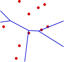
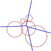
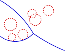
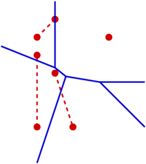
Figure 5.3: Farthest-site Voronoi diagrams of the same sites as in Figure 1.2, computed with our software. 5.3 A farthest point Voronoi diagram. 5.3 A farthest additively-weighted Voronoi diagram. 5.3 A farthest Möbius diagram. 5.3 A farthest Voronoi diagram of segments. The sites in 5.3, 5.3, and 5.3 are illustrated with dashed curves.

Given a traits class for nearest Voronoi diagrams, our framework enables the immediate computation of the respective farthest Voronoi diagrams (using the CGAL::farthest_voronoi_2 function — see Section 3.3). The construction of the upper envelope of the distance functions from the sites yields the farthest Voronoi diagram. Figure 5.3 shows various farthest-site Voronoi diagrams computed with our framework.

Post-computation Operations

Voronoi diagrams are represented as exact Cgal arrangements, and their vertices, edges, and faces can easily be traversed while obtaining the coordinates of the vertices of the diagram to any desired precision, if the situation requires.

Most applications require additional operations to be performed on the resulting Voronoi diagrams. The computed diagrams can be passed as input to consecutive operations supported by the Arrangement_on_surface_2 package and its derivatives. We get plenty of additional functionalities for free. Among those are (i) point-location queries and vertical-ray shooting, (ii) the ability to perform aggregated insertion of additinal curves, (iii) computing the zone of a curve inside a Voronoi diagram and inserting a curve in an incremental fashion to an existing diagram, (iv) the ability to remove existing edge of the diagram, (v) overlaying two (or more) Voronoi diagrams or arrangements, (vi) the ability to attach user-defined data to all of the geometric and topological primitives, and (vii) the ability to use the Boost graph library to run various graph algorithms on the diagram and its dual structure [cgal:wfzh-a2-08]. There are specific applications for the overlay of Voronoi diagrams, for example, representing the local zones of two competing telecommunication operators [bgz-spvt-00]. We describe an application of the overlay operation for computing a minimum-width annulus of a set of disks in the plane in Chapter 6.

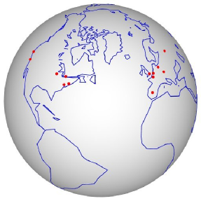
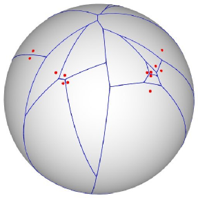
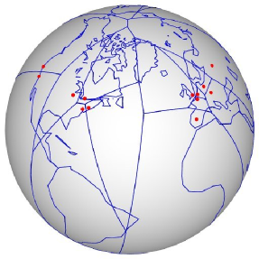
Figure 5.4: Overlaying an arrangement and a Voronoi diagram on the sphere. 5.4 Arrangement induced by the continents and some of the islands on earth. 5.4 Voronoi diagram of 20 points on the sphere representing 20 major cities on the planet. 5.4 The overlay of the arrangement from 5.4 and the Voronoi diagram from 5.4.

Figure 5.4 shows an arrangement on the sphere induced by (i) the continents and some of the islands on earth, and (ii) 20 major cities in the world, which appear as isolated vertices. The arrangement consists of 1065 vertices, 1081 edges, and 117 faces. The initial data was taken from gnuplot gnuplot-link and google maps googlemaps-link. The middle sphere embeds an arrangement that represents the Voronoi diagram of the 20 cities above. The right figure shows the overlay of the two aforementioned arrangements computed with the generic overlay function from the Arrangement_on_surface_2 package.

5.2 Limitations

Practical Computation Time

Theoretically, the randomized divide-and-conquer envelope approach for computing Voronoi diagrams is efficient and is asymptotically comparable to other (near-)optimal methods. Practically, however, the concrete running time of our implementation is inferior to those of existing implementations of various dedicated implementations (for specific type of diagrams). Following are possible explanations for the gap.

1. The method uses constructions of bisectors and Voronoi vertices as elementary building-blocks and they must be exact. Geometric algorithms based on constructors (rather than predicates) are usually more time and space consuming, especially when the constructed objects are exact, like in our case.

2. Each face of the overlay is inspected during the merge step. Though randomization ensures us that the expected number of faces is proportional to the complexity of the final diagram, a large number of redundant faces is being examined. Other algorithms do not examine all the faces of the overlay, for example, the classic algorithm by Shamos and Hoey [sh-cpp-75] suggests that by sorting the input point sites only a small number of faces has to be handled. Our general framework is unaware of these kind of optimizations that relate to the specific type of the Voronoi diagram.

3. In many dedicated Voronoi diagrams algorithms implementations, various optimizations are employed to reduce the running time of the algorithm. Most of these optimizations cannot be applied by the general algorithm. For example, some Voronoi diagrams algorithms harness the fact that sites usually affect only their surroundings to optimize the code. Our general algorithm cannot assume such a thing.

Our work can be probably improved further, but it is reasonable to assume that the general implementation will continue to be inferior to other implementations.

Bisector Construction

Besides affecting the time performance of the algorithm, constructing and manipulating bisectors have other limitations. In certain cases, it is hard to construct the bisector of two sites. The bisector could be two-dimensional or composed of several arcs, and the efficient construction of it may not be trivial. The user does not need to know the details of constructing lower envelopes of distance functions, indeed, but he/she may have to posses fairly advanced knowledge in computational algebra.

In other cases, there may not be an existing traits class for the arrangement package that supports the construction of an arrangement induced by the bisector curves. The user may have to create a traits class for the arrangement package themselves.

One can also imagine diagrams that will not be supported by the framework due to the hardness of the computation of their bisectors. For example, it is not clear what is the type of the curves that constitute the boundaries of the cells of the zone diagram [amt-zdeuac-07].

Incremental Construction and Removal

Incremental insertion of Voronoi sites could be very useful [obsc-stcavd-00, mgd-diovdm-03], for example, for developing online Voronoi diagrams’ construction algorithms. Our framework can support the insertion of a single site by partitioning the input to one set that consists of $n-1$ sites and another set that consists of a single site. Unfortunately, this insertion procedure is expected to be most inefficient. The current implementation will try and bisect each of the faces with the bisector of the new site and the dominant site on the face, which will result in $\Omega(n)$ time per insertion operation.

A deletion operation of sites is also useful [d-ddt-02, mgd-diovdm-03] but is not supported by the framework. Adding this operation to the framework is not trivial.

Chapter 6 Application: Minimum-Width Annulus of Disks

In this chapter we describe the application of our framework to solve the problem of computing a minimum-width annulus of a set of disks in the plane. Our algorithm is a generalization of a known algorithm for computing a minimum-width annulus of a set of points in the plane, and its implementation exploits the generality and the flexibility of our framework. Section 6.1 gives a short introduction and background on the problem. Section 6.2 presents our generalized algorithm. Finally, Section LABEL:sec:min-annulus:impl gives specific implementation details and experimental results for the application.

6.1 Introduction

An annulus is the bounded area between two concentric circles. The width of an annulus is the difference between the radii of the outer circle and the inner circle. Given a set of objects in the plane the objective is to find a minimum-width annulus containing those objects.

Constructing a minimum-width annulus of a set of points has applications in diverse fields. We list below two examples, taken from the areas of tolerancing metrology and facility location; more applications can be found in [bbbrw-ccmwap-98, cd-fdtcpr-09] and other papers.

In the field of mechanical design, assessing the deviation of a manufactured object from its ideal design is a key problem. If the manufactured object is round then this deviation is called the roundness error of the object. When assessing the roundness error of a manufactured object, four types of roundness errors are most commonly used, that is Maximum Inscribed Circle, Minimum Circumscribing Circle, Least Squares Center, and Minimum Radial Separation (MRS). The MRS roundness error is defined to be the minimum difference between the radii of two concentric circles (one circumscribing and one inscribed). Therefore, computing the MRS roundness error amounts to computing a minimum-width annulus containing the points sampled from the manufactured object [y-ecgtm-94].

Facility location generally deals with the placement of facilities for minimizing costs under various restrictions. When considering a location for a new facility among existing facilities, in many cases the most “fair” location is the location where the difference between the maximal and the minimal effects on existing facilities is brought to a minimum [ms-emflar-94]. In other cases, facilities may have both desirable and obnoxious properties. For example, the service area of a cell site should cover the locations of its clients, and due to aesthetic and health constraints, should preferably be in the farthest location possible from all clients. In both cases the center of a minimum-width annulus containing the locations of the existing facilities and the locations of the clients, respectively, is a good location.

A minimum-width annulus does not always exist. If the width of the set of objects is smaller than the width of any containing annulus, then there is no minimum-width annulus. Consider, for example, four collinear points in the plane. For every annulus containing the four points, we can always find another annulus with smaller width by moving the center of the original annulus away from the points on the line perpendicular to the line passing through them.

In the case of point sets, the minimum-width annulus must have (at least) two points on its outer circle and (at least) two points on its inner circle [r-ac-79, sr-wrspp-99], which results in the following observation:

Observation 6.1.

The center of a minimum-width annulus of points in the plane must lie on an intersection point of the nearest-site Voronoi diagram and the farthest-site Voronoi diagram of the points.

The center of an empty circle touching (at least) two points is on an edge of the nearest-site Voronoi diagram of the points, and the center of a circle containing all the points and touching (at least) two points is on an edge of the farthest-site Voronoi diagram.

Using the above observation, Ebara et al. [efnn-ravd-89] gave a worst-case $O(n^{2})$ time algorithm for finding a minimum-width annulus of points in the plane. The algorithm was reintroduced to the manufacturing community by Roy and Zhang [rz-epccm-92].

Similar methods were used to solve different variations of the problem. de Berg et al. [bbbrw-ccmwap-98] used nearest-site and farthest-site Voronoi diagrams to compute a minimum-width annulus of point sets with various constraints on its radii (e. g., fixed inner radius). Le and Lee [ll-orpr-91] showed how to use the overlay of the medial axis of a simple polygon (which is the Voronoi diagram of its edges restricted to the interior of the polygon) and the farthest Voronoi diagram of the vertices of the polygon to compute a minimum-width annulus bounding the polygon. Barequet et al. considered several problems and applied similar techniques for the case of offset-polygon annuli containing a set of points [bbdg-opapp-98, bbdg-occpa-05].

For special cases there are deterministic sub-quadratic algorithms. Garcia-Lopez et al. [lrs-fspc-98] showed that given the final circular order of the points around the center of the annulus (not a far-fetched scenario in real-world applications), a minimum-width annulus can be found in worst-case time complexity of $O(n\log n)$. Swanson et al. [slw-oardc-95] introduced an optimal $O(n)$ time algorithm for computing the roundness of convex polygons. Devillers and Ramos [dr-cresar-02] gave an algorithm that exhibits linear running time in practice for point-sets that are almost round.

Several randomized sub-quadratic algorithms exist for finding a minimum-width annulus of points in the plane [aas-cefda-97, as-erasgo-96, tas-apsgo-94]. The algorithm by Agarwal and Sharir [as-erasgo-96] achieves an expected running time of $O(n^{3/2+\varepsilon})$ which is the best known algorithm to date. Using core-sets Chan [c-fcscd-06] presented an $(1+\varepsilon)$-factor approximation algorithm for the minimum-width annulus, improving previously known results [aaps-aamwas-00, ahv-aemp-04, c-adwsec-02].

In this chapter we describe an application of our framework that demonstrates its usefulness. We use our tools to find a minimum-width annulus containing a set of disks in the plane. Section 6.2 deals with the theoretical aspect of our algorithm. Section LABEL:sec:min-annulus:impl describes major implementation details and some experimental results.

6.2 Algorithm for Minimum-Width Annulus of Disks

As mentioned above, when dealing with point sets, a minimum-width annulus can be found by computing the overlay of the nearest-site and farthest-site Voronoi diagrams of the points. A similar approach applies to the case of disk sites but the diagrams have to be defined more carefully.

Consider the following farthest-point distance function from a point $p\in{\mathbb{R}}\rule{0.85358pt}{0.0pt}^{2}$ to a set of points $S\subset{\mathbb{R}}\rule{0.85358pt}{0.0pt}^{2}$:

$$f(p,S)=\sup_{x\in S}{||p-x||},$$

which measures the farthest distance from the point $p$ to the set $S$. Consider the farthest-site Voronoi diagram with respect to this distance function. We call this diagram the “farthest-point farthest-site” Voronoi diagram. The distance function $f(p,S)$ becomes the Euclidean distance when the set $S$ consists of a single point. However, this is not the case when the set $S$ is, say, a disk in the plane.

The following observation establishes a connection between the farthest-point farthest-site Voronoi diagram of a set of disks and an additively-weighted Voronoi diagram, and comes in handy below.

Observation 6.2.

Let ${\mathcal{D}}$ be a set of disk in ${\mathbb{R}}\rule{0.85358pt}{0.0pt}^{2}$. The farthest-point farthest-site Voronoi diagram of ${\mathcal{D}}$ is identical to the Apollonius diagram of the disks with negated radii.

For a disk $d$ in the plane with center $c$ and radius $r$ the farthest-point distance function is $\rho(p,d)=||p-c||+r$. Recall that the Apollonius distance function is defined to be $\rho(p,d)=||p-c||-r$. Next, observe that the farthest-point distance function is the same as the Apollonius distance function with negative radii.

We prove that there is a minimum-width annulus (in case one exists) whose center is a vertex of the overlay of the Apollonius diagram and the farthest-point farthest-site Voronoi diagram of the disks.

Recall that in the case of point sets the center of a minimum-width annulus is an intersection point of the nearest-site Voronoi diagram and the farthest-site Voronoi diagram of the points. In the case of disks, this is not true. Take for example a set of disks located at $(2,0)$, $(0,3)$, $(-4,0)$, and $(0,-5)$ with radii $1$, $2$, $3$, and $4$, respectively. In this setting, the annulus centered at the origin with radii $1$ and $9$ is a minimum-width annulus, as its width is equal to a diameter of one of the disks. The origin does not lie on an edge of the farthest-point farthest-site Voronoi diagram, as the outer circle touches only one disk.

Let ${\mathcal{D}}{}=\{d_{1},\ldots,d_{n}\}$ be a collection of disks in the plane such that for all $i$, $d_{i}\not\subseteq\bigcup_{j\neq i}d_{j}$. For simplicity of exposition, we assume here that $n\geq 3$; the case of $n<3$ is simple to handle. We show that there is a minimum-width annulus whose bounding circles intersect the disks of ${\mathcal{D}}$ in at least 4 points.

Observation 6.3.

If ${N}$ is a minimum-width annulus containing ${\mathcal{D}}$ then each of the inner circle and the outer circle of ${N}$ touches a disk of ${\mathcal{D}}$.

Each minimum-width annulus must touch the disks of ${\mathcal{D}}$ in at least two points, as we can shrink the outer circle of the annulus and expand the inner circle until each of them touches a disk. Thus, fixing a point $p$ in the plane as the center of a containing annulus fixes an annulus bounding ${\mathcal{D}}$ for this center. We call this annulus the tight annulus fixed at $p$.

Let ${N_{p}}$ denote the tight annulus fixed at point $p$ and let ${W_{{N_{p}}}}$ denote its width. Let ${\mathcal{I}}_{p},{\mathcal{O}}_{p}\subseteq{\mathcal{D}}$ denote the set of disks that are touched by the inner and outer circles of ${N_{p}}$, respectively.

Definition 6.4 (Neighboring center in direction $\vec{d}$).

For a point $p$ and a direction $\vec{d}$ in the plane, consider the ray $r$ emanating from $p$ in direction $\vec{d}$. $r$ can be divided into maximally-connected cells, such that every point $x$ in a cell ($x$ is the center of a tight annulus) obtains the same ${\mathcal{I}}_{x}$ and ${\mathcal{O}}_{x}$. Let $p^{\prime}$ be an interior point of the cell of $p$, or, if $p$ comprises a single-point cell, an interior point of the next cell in the direction of the ray. We call $p^{\prime}$ a neighboring center of $p$ in direction $\vec{d}$.