Log-Poisson Cascade Description of Turbulent Velocity Gradient Statistics

Abstract

The Log-Poisson phenomenological description of the turbulent energy cascade is evoked to discuss high-order statistics of velocity derivatives and the mapping between their probability distribution functions at different Reynolds numbers. The striking confirmation of theoretical predictions suggests that numerical solutions of the flow, obtained at low/moderate Reynolds numbers can play an important quantitative role in the analysis of experimental high Reynolds number phenomena, where small scales fluctuations are in general inaccessible from direct numerical simulations.

I Introduction

Since the pioneering experimental work of Batchelor and Townsend, published exactly sixty years ago batch-town it is known that scale dependent galilean invariant observables, like velocity differences, fluctuate in a strongly non-gaussian way at small scales in turbulent flows. This kind of statistical behavior, generally referred to as “intermittency”, indicates that the K41 picture of turbulence k41a ; k41b , which actually would correspond to the existence of a homogeneously distributed energy dissipation field frisch2 , should break down, a fact notoriously anticipated by Landau as early as in 1942 frisch1 . Not less remarkably, long before additional breakthrough experiments were performed ansel_etal , phenomenological models of the energy cascade advanced the conjecture that intermittency should be related to the stochastic multiplicative nature of the energy cascade process k62 ; ob62 , implying that small scale strong fluctuations are, in some sense, fed by the weaker large scale ones.

The intermittency phenomenon is commonly associated with the anomalous scaling of velocity structure functions. A comprehensive description dealing with both anomalous scaling and the non-gaussian behavior of intermittent observables is a major challenge of three-dimensional turbulence theory tsinober . Small scale strong fluctuations are believed to reflect the dynamics of coherent structures like vortex filaments. Even though this is a very open problem, a similar physical picture is in fact well-established in simpler contexts, as in Burgers turbulence bec , with shocks playing the role of “vortices”.

The log-Poisson model dubrulle ; she yields perhaps the most intriguing description of the turbulent multiplicative cascade, since, as it is well-known, it leads to the accurate She-Leveque intermittency exponents of velocity structure functions she-leveque . The phenomenological work of She and Leveque is also of great physical appeal, once it places vortex filaments as a fundamental ingredient in the production of intermittency.

We are interested, in this work, to know what the log-Poisson model may tell us about the profiles of velocity gradient pdfs. We deal here with two sets of pdfs for flows associated to different Reynolds numbers. One of them is obtained from an atmospheric surface layer experiment guli1_etal ; guli2_etal ; guli3_etal and the other from a direct numerical simulation (DNS) of homogeneous and isotropic turbulence donzis . The underlying motivation in this choice of systems is to show that numerical low/moderate Reynolds number results can be useful in the modelling of flows that cannot be directly simulated (even in a foreseeable future). The very same claim was put forward in a previous letter kholmy , where, despite the force of evidence, lacked some phenomenological basis, which, then, we develop here. We find that a bridge between low and high Reynolds number pdfs can be built within the framework of the log-Poisson model comment .

This paper is organized as follows. In Sec. II we briefly review the multiplicative cascade models, introduce the log-Poisson model and compute hyperflatness factors of velocity gradient fluctuations, comparing them to recent estimates. Two relevant theorems related to velocity gradient pdfs are also established. In Sec. III, we present the experimental and numerical data that was analysed. In Sec. IV, the experimental and the numerical velocity gradients are closely matched with the help of a Monte-Carlo procedure based on the theorems of Sec. II. In Sec. V, we summarize our results and point out directions of further research.

II Velocity Gradient Statistics

Multiplicative Cascade Models

In the multiplicative cascade models frisch2 , one assumes that energy flows from the integral scale $L$ to the dissipative scale $\eta$ through a number of “quantum” steps associated to eddies of sizes $L,L/a,L/a^{2},...$, where $a>1$ is an arbitrary rescaling factor. At length scale $\ell_{m}\equiv L/a^{m}$ the fluctuating energy transfer rate is defined as

$$\epsilon_{m}=\epsilon_{0}W_{1}W_{2}...W_{m}\ ,\$$ (1)

where the $W$’s are positive independent random variables, with unit expectation value, $\langle W\rangle=1$, so that the mean energy transfer rate is conserved along the cascade process, i.e., $\langle\epsilon_{m}\rangle=\epsilon_{0}$. The scaling behavior of velocity structure functions, $S_{q}(r)\equiv\langle(\delta v)^{q}\rangle$ is, then, derived with the help of Kolmogorov’s refined similarity hypothesis, which postulates that fluctuations of $\delta v$ at scale $\ell_{m}$ have the same moments (up to constant numerical factors) as $(\epsilon_{m}\ell_{m})^{1/3}$.

Analogous phenomenological arguments can be put forward to deal with the case of velocity derivatives – generically denoted in the following by $\partial v$. The essential idea is to assume that spatial fluctuations of the velocity field are smooth at the dissipative scale, and, therefore,

$$\partial v\sim\frac{\delta v_{\eta}}{\eta}\sim(\epsilon_{\eta})^{1/3}\eta^{-2/3}\ ,\$$ (2)

where, above, $\delta v_{\eta}$ is the velocity increment defined at length scale $\eta$. One may write, based on purely dimensional grounds, $\eta\sim(\nu^{3}/\epsilon_{\eta})^{1/4}$. Thus, substituting the latter on (2), we get

$$\partial v\sim\sqrt{\epsilon_{\eta}/\nu}\ ,\$$ (3)

a statistical correspondence not unknown to the previous literature wyn-tenn . A more interesting formulation of the refined similarity hypothesis is given in terms of probability distributions. As it is clear, velocity gradient pdfs can be always written as

$$\rho(\partial v)=\int_{0}^{\infty}d\epsilon\rho_{1}(\epsilon)\rho_{2}(\partial v|\epsilon)\ ,\$$ (4)

where $\rho_{2}(\partial v|\epsilon)$ is the velocity gradient pdf conditioned on the energy transfer rate $\epsilon_{\eta}=\epsilon$ and $\rho_{1}(\epsilon)$ is the pdf associated to events which have $\epsilon_{\eta}=\epsilon$. The refined similarity hypothesis is, then, the statement that at large Reynolds numbers,

$$\rho_{2}(\partial v|\epsilon)=\sqrt{\nu/\epsilon}F(\sqrt{\nu/\epsilon}\partial v)\ ,\$$ (5)

where $F(\cdot)$ is a universal (Reynolds number independent) function of its argument. In fact, taking (4) and (5), it is not difficult to show, in agreement with (3), that

$$\langle(\partial v)^{q}\rangle=C_{q}\langle(\epsilon_{\eta}/\nu)^{\frac{q}{2}}\rangle\ ,\$$ (6)

where

$$C_{q}=\int_{-\infty}^{\infty}dxx^{q}F(x)\ .\$$ (7)

It is worth noting that the form of the universal functions $F(x)$ for the case of velocity differences has been the subject of experimental research gagne ; naert . As a first approximation, $F(x)$ turns to have a gaussian profile, but one expects asymmetric corrections to be relevant in the problem of longitudinal structure functions, due to their non-vanishing skewness.

Log-Poisson Model

In the log-Poisson model dubrulle ; she one writes down the energy transfer rate factors as

$$W=a^{\mu-m}\ ,\$$ (8)

where $a=3/2$, $\mu=2/3$ and $m\geq 0$ is a Poisson random variable, with expectation value

$$c=\frac{a\mu}{a-1}\ln a=2\ln\left(\frac{3}{2}\right)\ .\$$ (9)

In order to cope with velocity gradient fluctuations, it is necessary to set up in first place the total number $N$ of cascade steps associated to the turbulent flow under scrutiny. In other words, we would like to find $N$, such that $\eta=L/a^{N}$. We stress that the multiplicative cascade description addressed here is far from being a rigorous framework, since we take the Kolmogorov scale $\eta\sim\epsilon_{\eta}^{-1/4}$ to be a fluctuacting quantity. Thus, $N$ should be defined, necessarily, from some averaging procedure. We adopt a simple prescription based on the definition of the Reynolds number as frisch2

$$R_{e}=\frac{L^{\frac{4}{3}}\epsilon_{0}^{\frac{1}{3}}}{\nu}=\left[\langle\left(\frac{L}{\eta}\right)^{4}\rangle\right]^{\frac{1}{3}}\equiv a^{\frac{4}{3}N}\ .\$$ (10)

Therefore, we find

$$N=\frac{3}{4}\log_{a}R_{e}\ .\$$ (11)

An alternative and useful expression for $N$ can be given in terms of the Taylor-based Reynolds number $R_{\lambda}$, which follows by taking the homogeneous isotropic result $R_{\lambda}=\sqrt{15R_{e}}$ frisch2 ,

$$N=\frac{6}{4}\log_{a}R_{\lambda}-\frac{3}{4}\log_{a}15\ .\$$ (12)

Hyperflatness Factors

As a direct application of the log-Poisson model, we compute the Reynolds-dependent velocity gradient hyperflatness factors, defined as

$$H_{q}(R_{\lambda})\equiv\frac{\langle(\partial v)^{q}\rangle}{\langle(\partial v)^{2}\rangle^{\frac{q}{2}}}\ .\$$ (13)

A straightforward manipulation of (13), taking into account (1), (6) and (8), gives

$$H_{q}(R_{\lambda})=\frac{C_{q}}{C_{2}^{\frac{q}{2}}}\langle\left(\frac{\epsilon_{\eta}}{\epsilon_{0}}\right)^{\frac{q}{2}}\rangle=\frac{C_{q}}{C_{2}^{\frac{q}{2}}}\langle W^{\frac{q}{2}}\rangle^{N}=A_{q}R_{\lambda}^{\alpha_{q}}\ ,\$$ (14)

where

$$A_{q}=\frac{C_{q}}{C_{2}^{\frac{q}{2}}}15^{-\frac{\alpha_{q}}{2}}\ ,\$$ (15)

with

$$\alpha_{q}=\frac{3}{2}\log_{a}\langle W^{\frac{q}{2}}\rangle=\frac{3}{4}q\mu-\frac{3}{2}\frac{a\mu}{a-1}[1-a^{-\frac{q}{2}}]\ .\$$ (16)

In particular, the skewness and flatness coefficients predicted by (16) are $\alpha_{3}\simeq 0.13$ and $\alpha_{4}=1/3$, respectively. Good support is found from the recent account of Ishihara et al. ishi_etal , which yields $\alpha_{3}=0.11\pm 0.01$ and $\alpha_{4}=0.34\pm 0.03$.

If $R_{A}$ and $R_{B}$ are Taylor-based Reynolds numbers, respectively associated to flows with $N_{A}$ and $N_{B}$ cascade steps, then (14) implies that

$$\frac{H_{q}(R_{A})}{H_{q}(R_{B})}=\langle W^{\frac{q}{2}}\rangle^{N_{A}-N_{B}}\ ,\$$ (17)

and, thus, taking into account (16),

$$N_{A}-N_{B}=\frac{3}{2\alpha_{q}}\log_{a}\frac{H_{q}(R_{A})}{H_{q}(R_{B})}\ ,\$$ (18)

a quantity that measures the “distance” between cascades, going to play an important role in Sec. IV.

Velocity Gradient PDFs

We are interested to explore further consequences of the log-Poisson cascade picture in the setting of velocity gradient pdfs. In order to render the exposition more systematic, we introduce two important results in the form of theorems.

Theorem 1.

Let $\sigma^{2}\equiv\langle(\partial v)^{2}\rangle$. The standardized pdf $\tilde{\rho}(\partial v)\equiv\sigma\rho(\sigma\partial v)$ has a universal profile at fixed $R_{\lambda}$.

Proof.

We obtain, from (4) and (5),

$$\tilde{\rho}(\partial v)=\sigma\rho(\sigma\partial v)=$$ (19)

$$= \sigma\int_{0}^{\infty}d\epsilon\rho_{1}(\epsilon)\sqrt{\nu/\epsilon}F(\sigma\sqrt{\nu/\epsilon}\partial v)$$

$$= \nu\sigma^{2}\int_{0}^{\infty}d\epsilon\rho_{1}(\nu\sigma^{2}\epsilon)\sqrt{1/\epsilon}F(\sqrt{1/\epsilon}\partial v)\ .\$$

Our task, thus, is to show that $\nu\sigma^{2}\rho_{1}(\nu\sigma^{2}\epsilon)$ is indeed universal. Since the sum of Poisson random variables is also a Poisson random variable, Eqs. (1) and (8) lead, for a cascade with $N$ steps, to

$$\epsilon_{\eta}=\epsilon_{0}a^{N\mu-m}\ ,\$$ (20)

where $m$ is a Poisson random variable with expectation value $Nc$. We may write, thus,

$$\rho_{1}(\epsilon)=\sum_{m=0}^{\infty}\frac{(Nc)^{m}e^{-Nc}}{m!}\delta(\epsilon-\epsilon_{0}a^{N\mu-m})\ .\$$ (21)

Now, according to (6) we write the variance of $\partial v$ as $\sigma^{2}=\epsilon_{0}C_{2}/\nu$, and, therefore, find

$$\nu\sigma^{2}\rho_{1}(\nu\sigma^{2}\epsilon)=C_{2}\sum_{m=0}^{\infty}\frac{(Nc)^{m}e^{-Nc}}{m!}\delta(C_{2}\epsilon-a^{N\mu-m})\ ,\$$ (22)

which, in fact, ultimately depends only on $R_{\lambda}$.

∎

Theorem 2.

Let $A$ and $B$ denote flows with Taylor-based Reynolds numbers $R_{A}$ and $R_{B}$, associated to log-Poisson cascades with $N_{A}$ and $N_{B}$ steps, and velocity gradient pdfs

$$\rho_{A}(\partial v)=\int_{0}^{\infty}d\epsilon\rho^{A}_{1}(\epsilon)\sqrt{\nu/\epsilon}F(\sqrt{\nu/\epsilon}\partial v)\ ,\$$

$$\rho_{B}(\partial v)=\int_{0}^{\infty}d\epsilon\rho^{B}_{1}(\epsilon)\sqrt{\nu/\epsilon}F(\sqrt{\nu/\epsilon}\partial v)\ .\$$ (23)

It follows that

$$\tilde{\rho}_{A}(\partial v)=\int_{0}^{\infty}\frac{dx}{x}K(x)\tilde{\rho}_{B}(\frac{\partial v}{x})\ ,\$$ (24)

where $K(x)$ is the pdf of the random variable

$$x=a^{\frac{1}{2}(N_{A}-N_{B})\mu-\frac{m}{2}}\ ,\$$ (25)

which, on its turn, is defined in terms of $m$, a random Poisson variable with expectation value $(N_{A}-N_{B})c$.

Proof.

A proof follows by direct substitution of the explicit form of $K(x)$ in (24). Defining $g=a^{N\mu/2}$, with $N=N_{A}-N_{B}$, we may write

$$K(x)=\sum_{m=0}^{\infty}\frac{(Nc)^{m}e^{-Nc}}{m!}\delta(x-ga^{-\frac{m}{2}})\ .\$$ (26)

Using (22) and (26), we obtain, for the RHS of (24),

$$\int_{0}^{\infty}\frac{dx}{x}K(x)\tilde{\rho}_{B}(\frac{\partial v}{x})$$ (27)

$$= \int_{0}^{\infty}\frac{dx}{x}\sum_{m=0}^{\infty}\frac{(Nc)^{m}e^{-Nc}}{m!}\delta(x-ga^{-\frac{m}{2}})$$

$$\times \int_{0}^{\infty}d\epsilon\nu\sigma_{B}^{2}\rho_{1}^{B}(\nu\sigma_{B}^{2}\epsilon)\sqrt{1/\epsilon}F(\sqrt{1/\epsilon}\partial v/x)$$

$$= C_{2}\int_{0}^{\infty}\frac{dx}{x}\int_{0}^{\infty}d\epsilon\sum_{m=0}^{\infty}\sum_{m^{\prime}=0}^{\infty}\frac{(Nc)^{m}e^{-Nc}}{m!}$$

$$\times \frac{(N_{B}c)^{m^{\prime}}e^{-N_{B}c}}{m^{\prime}!}\delta(x-ga^{-\frac{m}{2}})\delta(C_{2}\epsilon-a^{N_{B}\mu-m})$$

$$\times \sqrt{1/\epsilon}F(\sqrt{1/\epsilon}\partial v/x)\ .\$$

Performing the substitution $\epsilon\rightarrow\epsilon/x^{2}$ in (27) and subsequently integrating over $x$, we get

$$C_{2}\int_{0}^{\infty}d\epsilon\sum_{m=0}^{\infty}\sum_{m^{\prime}=0}^{\infty}\frac{(Nc)^{m}(N_{B}c)^{m^{\prime}}e^{-N_{A}c}}{m!m^{\prime}!}$$

$$\times \delta(C_{2}\epsilon-g^{2}a^{N_{B}\mu-m-m^{\prime}})\sqrt{1/\epsilon}F(\sqrt{1/\epsilon}\partial v)\ .\$$

Define, now, $p=m+m^{\prime}$, so that (LABEL:eq2.28) becomes

$$C_{2}\int_{0}^{\infty}d\epsilon\sum_{p=0}^{\infty}\sum_{m=0}^{p}\frac{(Nc)^{m}(N_{B}c)^{m-p}e^{-N_{A}c}}{m!(m-p)!}$$ (29)

$$\times \delta(C_{2}\epsilon-g^{2}a^{N_{B}\mu-p})\sqrt{1/\epsilon}F(\sqrt{1/\epsilon}\partial v)$$

$$= C_{2}\int_{0}^{\infty}d\epsilon\sum_{p=0}^{\infty}\frac{(N_{A}c)^{p}}{p!}e^{-N_{A}c}\delta(C_{2}\epsilon-a^{N_{A}\mu-p})$$

$$\times \sqrt{1/\epsilon}F(\sqrt{1/\epsilon}\partial v)=\tilde{\rho}_{A}(\partial v)\ .\$$

∎

In view of Theorem 2 we can devise a straightforward Monte-Carlo integration procedure in order to relate velocity-gradient pdfs defined at different Reynolds numbers. In fact, if $x>0$ and $y$ are random variables of two independent stochastic process, described, respectively, by pdfs $K(x)$ and $\tilde{\rho}(y)$, then the random variable $z=xy$ is given by the pdf

$$\langle\delta(z-xy)\rangle_{x,y} = \int dxdyK(x)\tilde{\rho}(y)\delta(z-xy)$$ (30)

$$= \int_{0}^{\infty}\frac{dx}{x}K(x)\tilde{\rho}(\frac{z}{x})=\tilde{\rho}(z)\ ,\$$

where we have used (24) in the last equality above. We have found that it is greatly advantageous to use Monte-Carlo integration, instead of more traditional numerical methods, a fact probably due to the bad convergence properties of the latter in our particular problem.

III atmospheric surface Layer Experiment

Atmospheric surface layer velocity fluctuations were studied over a grass-covered flat surface in the Sils-Maria valley, Switzerland guli1_etal , a place which hosts reasonably stable winds. The results reported in this work correspond to measurements of all of the nine components of the velocity gradient tensor, performed in a tower 3.0 m high. The velocity signal was recorded at sampling rate of $10$ KHz (which was high enough to resolve the dissipative scales), with the help of a 20 hot-wire probe anemometer, specifically designed for the particularities of the field experiment.

Figure 1: Experimental velocity gradient pdfs for atmospheric surface layer flow with $R_{\lambda}=3.4\times 10^{3}$. Black line: $s_{11}$; collored lines: $s_{ij}$, with $i\neq j$.

Figure 2: Numerical velocity gradient pdfs for homogeneous isotropic turbulence with $R_{\lambda}=240$. Black lines: diagonal components $s_{ii}$; red lines: non-diagonal components $s_{ij}$.

Figure 3: Comparison between the numerical ($R_{\lambda}=240$; solid line) and the experimental ($R_{\lambda}=3.4\times 10^{3}$; dots) pdfs of $s_{11}$.

Figure 4: Comparison between the numerical ($R_{\lambda}=240$; solid line) and the experimental ($R_{\lambda}=3.4\times 10^{3}$; dots) pdfs of $s_{23}$.

Velocity gradients were computed without resort to the Taylor’s frozen turbulence hypothesis. The Taylor-based Reynolds number of the flow, estimated from the Taylor length $\lambda=\sqrt{u_{1}^{2}/\langle(\partial_{1}u_{1})^{2}\rangle}$ is $R_{\lambda}=3.4\times 10^{3}$ ($u_{1}$ is the projection of the velocity fluctuations along the flow direction). We note that since the flow is somewhat anisotropic, the definition of a meaningful Taylor-based Reynolds number may be problematic. We will get back to this point in Sec. IV.

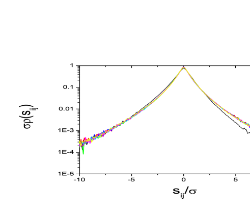
The experimental velocity gradient pdfs are shown Fig.1. We find a good (within error bars) collapse of standardized pdfs of velocity gradients $s_{ij}=\partial_{j}u_{i}$ with $i\neq j$. Due to anisotropy effects in the surface layer, however, there is no collapse for the standardized pdfs of diagonal components, $s_{ii}$, and we have discarded the curves for $s_{22}$ and $s_{33}$ assuming, as a working hypothesis to be tested a posteriori, that isotropic results would correspond to the set $\{s_{11},s_{ij}\}$, with $i\neq j$.

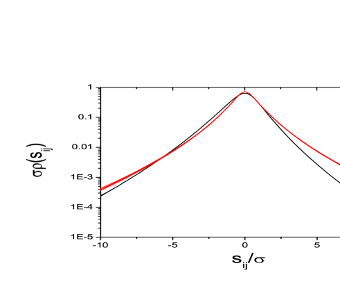
The central aim of this work is to model the pdfs depicted in Fig. 1 using direct numerical simulation (DNS) results for homogeneous and isotropic turbulence obtained at the considerably lower Taylor-based Reynolds number $R_{\lambda}=240$ (the numerical data corresponds to simulations discussed in Ref. donzis ). The corresponding DNS velocity gradient pdfs are shown in Fig. 2. As it follows from this figure, the pdfs collapse into two distinct groups, associated to the diagonal and non-diagonal components of the velocity gradient tensor $s_{ij}$. Of course, we do not expect that the pdfs given in Fig. 2 yield a direct fitting to the ones of Fig. 1 – there is a clear discrepancy as shown in Figs. 3 and 4.

IV Monte-Carlo PDF Reconstruction

Our computational strategy is to consider the experimental ($R_{\lambda}=3.4\times 10^{3}$) and the numerical ($R_{\lambda}=240$) flows discussed in Sec. III as the systems $A$ and $B$, respectively, of Theorem 2. An important parameter here is the cascade distance $N_{A}-N_{B}$ of these flows. This quantity can be computed by measuring the flatness factors $H_{4}$ of flows $A$ and $B$ and using them as input parameters in (18). From the pdfs of $s_{11}$, we get

$$H_{4}(A) = 11.5\ ,\$$

$$H_{4}(B) = 6.6\ .\$$ (31)

Therefore, using (18), with $\alpha_{4}=1/3$, we find

$$N_{A}-N_{B}=\frac{9}{2}\log_{\frac{3}{2}}\left(\frac{11.5}{6.6}\right)=6.16\ .\$$ (32)

Due to the discrete structure of the cascade in the multiplicative models, we take $N_{A}-N_{B}=6$ in the following considerations.

Figure 5: The numerically reconstructed pdf of $s_{11}$ (black solid line) is compared to the experimental pdf (red circles).

Figure 6: The numerically reconstructed pdf of $s_{23}$ (black solid line) is compared to the experimental pdfs of $s_{ij}$, with $i\neq j$ (collored symbols).

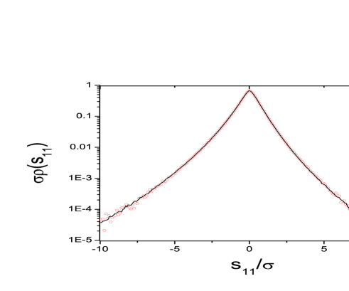
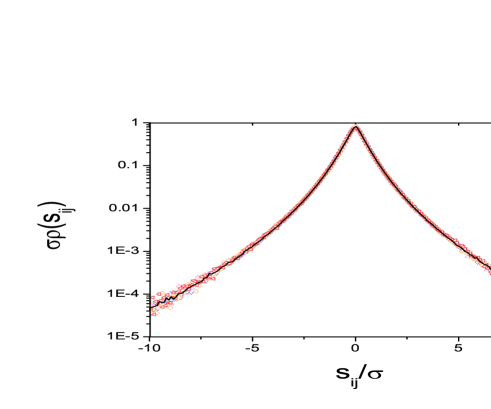
Using a random Poisson variable generator as the one given in Ref. knuth , it is straightforward to establish a stochastic process with random variable given by (25). On the other hand, in order to generate a stochastic process with random variable described by the numerical pdf of $s_{11}$, we proceed in two steps: first, we define an accurate polynomial fitting to the $\log_{10}\tilde{\rho}_{B}(s_{11})$ profile; second, the polynomial analytical distribution just obtained is used in a Monte-Carlo accept-reject algorithm mc , which produces random variables distributed according to $\tilde{\rho}_{B}(s_{11})$. Analogous computations are performed for the numerical pdfs of $s_{23}$, which are taken as a representative of the non-diagonal components of the velocity gradient tensor. By multiplying the stochastic processes associated to the Poisson and the numerical pdfs we get standardized pdfs which would hopefully fit the experimental curves. We have taken a process with $2\times 10^{7}$ elements. In fact, an excellent agreement is attained from the Monte-Carlo reconstructed pdfs, as shown in Figs. 5 and 6. A comparison between the modelled and the experimental pdfs is also shown in Figs. 7 and 8 in linear scales, to be contrasted to Figs. 3 and 4.

Figure 7: The numerically reconstructed pdf of $s_{11}$ (solid line) is compared to the experimental pdf (dots) in linear scales.

Figure 8: The numerically reconstructed pdf of $s_{23}$ is compared to the experimental pdf (dots) in linear scales.

It is important to emphasize that the remarkable fittings shown in Figs. 5-8, between the numerical and experimental pdfs for the set $\{s_{11},s_{ij}\}$, are obtained from the mapping, determined by the single parameter $N_{A}-N_{B}$, provided by the fluctuations given by (25). This constitutes strong evidence for the existence of an underlying log-Poisson cascade process. We note, furthermore, that the agreement between modelled and experimental pdfs would be not so good if the experimental pdfs of $s_{22}$ or $s_{33}$ were chosen in place of the one for $s_{11}$. The present method, thus, has the heuristic potential to address issues of isotropy in boundary layer flows.

A further application of our results is the definition of an effective Reynolds number $\bar{R}_{\lambda}$ for the atmospheric surface turbulent flow, taking the more controlled Reynolds number of the DNS as a standard. We write, according to (14),

$$\bar{R}_{\lambda}=240\times\left(\frac{11.5}{6.6}\right)^{3}\simeq 1.2\times 10^{3}\ .\$$ (33)

It was noted, in Ref. guli1_etal , that the rough estimate $R_{\lambda}=3.4\times 10^{3}$ displaces the point $(R_{\lambda},H_{4})=(3.4\times 10^{3},11.5)$ out of the empirical curve well modelled $H_{4}\sim R_{\lambda}^{\alpha_{4}}$. However, we find that if the alternative value (33) is used instead of $R_{\lambda}=3.4\times 10^{3}$, then the point $(R_{\lambda},H_{4})$ gets closer to the usual curve of flatness.

V Conclusions

We have used the log-Poisson model of the turbulent cascade to get the pdfs of velocity gradient fluctuations of a high Reynolds turbulent atmospheric flow. The excellent fittings are achieved by means of a Monte-Carlo integration procedure and the use of standard pdfs obtained in a lower Reynolds number DNS. Our results indicate that non-gaussianity and anomalous scaling of scale dependent observables can be seen as different manifestations of intermittency that can be approached within a unified framework. Actually, this point of view has been formerly pursued along the multifractal description of intermittency benzi1 , with modest success in the quality of pdf fittings, nevertheless the fact that they are dependent on a large number of free parameters.

As a natural application of our methodology, we have found a way to (i) select isotropy sectors of the velocity gradient tensor in boundary layer flows and (ii) unambiguously define effective Taylor-based Reynolds numbers in the presence of anisotropy. These results can be of considerable interest in the study of anisotropy effects in turbulent boundary layers. It is also likely that the same ideas can be extended to the case of free shear turbulence.

An interesting question is how low can be the DNS Reynolds number, while still leading to good velocity gradient pdf fittings for higher Reynolds number flows, along the lines discussed in Sec. IV. An investigation of this matter could throw some light on the problem of extended self-similarity benzi2 . Also, we wonder if correlation effects in the velocity gradient time series could be modelled in similar ways. A promising direction here would be to link the Fokker-Planck approach to turbulent time series peinke with the log-Poisson cascade model.

It is clear that the multiplicative cascade picture is worth as a phenomenological construction if a consistent meaning can be given to concepts like the inertial range, local cascade, and the universality of velocity structure exponents. However, recent work kholmy2 on the scaling behavior of velocity structure functions suggests that inertial and dissipative range fluctuations could be coupled in a bidirectional way. It has been found in kholmy2 that the scaling exponents measured in the inertial range are changed if strong dissipative events are discarded in the averaging procedure, indicating a “flow of influence” from the small to the large scales.

In order to address further related studies, we note that a possible solution to these puzzling observations, saving the essence of the multiplicative cascade phenomenology, would rely on the usual definition of the energy dissipation rate $\epsilon_{m}$ as the local dissipation rate averaged over volumes with linear sizes of the order of $\ell_{m}=L/a^{m}$. Since the energy dissipation rate is long-range correlated, it is likely that events which have strong local dissipation rates turn to be correlated to strong events in the above (inertial range averaged) sense.