Topological Peierls Transitions in Möbius Molecular Devices

Abstract

We study the topological properties of Peierls transitions in a monovalent Möbius ladder. Along the transverse and longitudinal directions of the ladder, there exist plenty Peierls phases corresponding to various dimerization patterns. Resulted from a special modulation, namely, staggered modulation along the longitudinal direction, the ladder system in the insulator phase behaves as a “topological insulator”, which possesses charged solitons as the gapless edge states existing in the gap. Such solitary states promise the dispersionless propagation along the longitudinal direction of the ladder system. Intrinsically, these non-trivial edges states originates from the Peierls phases boundary, which arises from the non-trivial $\mathbb{Z}^{2}$ topological configuration.

I INTRODUCTION

Many recent efforts have been made to both experimental and theoretical investigations of the application oriented molecular devices MD1 . As new type of the quantum coherence devices, molecular device emerges various novel quantum effects, which enlarge the ranges of the material design device1 ; device2 ; device3 ; device4 . In these systems, the exotic quantum features would be induced by the non-trivial topology, and the observable quantum effects can also be used to specify the topological constructions of the system. Indeed, this non-trivial topology induced quantum effects never appear in the topologically trivial systems.

With non-trivial topology, the twisted boundary condition in the Möbius strip is a good subject to demonstrate the significant role of topological structure in low-dimensional physics MBC1 ; MBC2 . The Möbius strip is a non-orientable manifold, whose edge defines a two-point bundles over $\mathbf{S^{1}}$ and thus $\mathbb{Z}^{2}$ topological configuration. This simple but topologically non-trivial system possesses mathematically rigorous description and the accessibilities of the experimental realization. Actually, the Möbius boundary condition has been synthesized in the aromatic annulenes, nanographite ribbons and conjugated polymers MS1 ; MS2 ; MS3 ; MS4 ; MS5 . These progresses motivate us to propose a tight-binding quantum device with Möbius topology and investigate its quantum properties of the transportation of the spinless particles Zhao ; Guo .

Another important phenomenon in molecular devices phonon1 ; phonon2 is their Peierls instability, which exists universally in low-dimensional physical system including polymers, spin chains, and organic materials, etc PT1 ; PT2 . The significance of the Peierls transition is that after the lattice is deformed due to the electron-phonon coupling, the system energy is decreased and thus the changed energy band structure converts the original metal phase into an insulator one. Actually, the existence of metal-insulator transition in the polyacetylene PT1 ; PT2 originates from this lattice modulation.

For the Möbius ladder configuration as a quasi-one dimensional (Q1D) system, investigation of the Peierls transitions apparently combines both the topological effect and the structure instability. In this paper, we demonstrate the various dimerization patterns in the monovalent Möbius ladder in details. Because of the possibilities of the lattice deformations along transverse and longitudinal directions, there exist five typical uniform dimerization patterns that we will display in this paper. In contrast, it is noticed that there is only one dimerization pattern in a one dimensional system. All the five dimerization patterns contain the rung, the columnar, the staggered dimerization patterns and the vertically saw-toothed, the inclined saw-toothed dimerization patterns as the combinations of the former three ones, all of which will be explicitly defined in the next section.

We compare the Peierls phase diagrams of the Möbius ladder with that of the generic one. Here, the generic ladder satisfies periodic boundary condition. It is discovered that when the generic boundary condition was replaced by a Möbius one, the conducting properties are dramatically changed for the staggered and the inclined saw-tooth dimerization patterns and not changed at all for the other three patterns. This fact motivates us to use the continuum model to analyze the exotic dimerizations. We notice the existence of the localized state ES1 ; ES2 , and find the charged solitons propagating in the bulk, which promise that the Möbius ladder with staggered dimerization is eventually metallic. Being similar to the gapless localized states in graphene strip, we also point out that our model behaves like a “topological insulator” TI1 ; TI2 with localized state existing at topological non-trivial boundary. Here, the topological insulator refers to a bulk insulator which possesses robust metallic localized states, which is different from mundane band insulator. These localized states are actually $\mathbb{Z}^{2}$ topologically invariant, which characterize the time-reversal invariance of the topological insulator.

This paper is organized as following. In Sec. II, we present the lattice Hamiltonian of the Möbius ladder and calculate the Peierls phase diagram. In comparison with the Möbius case, we also calculate the Peierls phase diagram of the generic ladder. To prove the existence of the non-trivial localized states, we introduce the continuum model of the Möbius ladder in Sec. III as well as the one of the generic ladder without any solitonary solution. We conclude our main results in Sec. IV. The detailed derivation of the continuum model from the lattice model is shown in Appendix A.

II TOPOLOGICAL PEIERLS TRANSITIONS AND CORRESPONDING PHASE DIAGRAM

II.1 Model setup and dimerization patterns

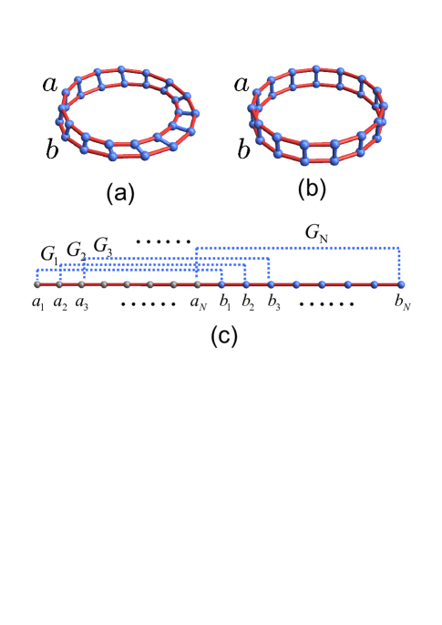
Figure 1: (Color online) Schematic illustrations of the ladder with (a) Möbius boundary condition, (b) generic boundary condition and (c) the corresponding one-dimensional version of Möbius ladder system with long range coupling.

In this section, we describe a tight binding model for the electrons hopping on a ladder with the tight-binding Hamiltonian

$$H_{\mathrm{e}}=\sum_{j=0}^{N-1}\mathbf{A}_{j}^{{\dagger}}\mathbf{M}_{j}\mathbf{A}_{j}-\sum_{j=0}^{N-1}\mathbf{J}_{j}\mathbf{A}_{j}^{{\dagger}}\mathbf{A}_{j+1}+h.c.,$$ (1)

where operator-value vectors $\mathbf{A}_{j}=(a_{j},b_{j})^{T}$ is defined in terms of the annihilation operator $a_{j}$ and $b_{j}$ of the upper and the lower chain of the ladder (see Fig. 1(a)), which are denoted as $a$-chain and $b$-chain in the following discussion. The transition matrices

$$\mathbf{M}_{j}=\varepsilon_{j}\sigma_{z}-G_{j}\sigma_{x}$$ (2)

and $\mathbf{J}_{j}=diag[J_{j}^{\mathrm{a}},J_{j}^{\mathrm{b}}]$ are defined by Pauli matrices $\sigma_{x},\sigma_{y}$ and $\sigma_{z}\mathbf{,}$ on-site energy differences $\varepsilon_{j}\equiv\varepsilon_{0},$ coupling strength between $a$-chain and $b$-chain $G_{j}\equiv G_{0}$ and hopping strength $J_{j}^{\mathrm{a}}=J_{j}^{\mathrm{b}}\equiv J_{0}.$ Here, $N$ is the site number of the $a$-($b$-)chain. To demonstrate the effect of the topology configuration of such system, we will consider two kinds of boundary conditions, which are the Möbius boundary condition characterized as

$$\mathbf{A}_{j+N}=\sigma_{x}\mathbf{A}_{j}$$ (3)

(see Fig. 1(a)) and the generic one characterized as

$$\mathbf{A}_{j+N}=\mathbf{A}_{j}$$ (4)

(see Fig. 1(b)).

The boundary condition apparently affects the system globally, and different boundary conditions result in different symmetries. The generic boundary condition corresponds to rotational symmetry, which implies the generic ladder possesses $S^{1}$ topological configuration. In contrast, the Möbius ladder is considered as a non-orientable manifold, whose edge defines a two-point bundle over $S^{1}$ and thus $Z^{2}$ topological configuration DG . This unusual topology can induce some novel effects such as induced gauge field and the cut-off of the electrons transmission spectrum Zhao . In our paper, the $Z^{2}$ topological configuration will contribute to the formation of the nontrivial localized states.

Figure 2: (Color online) Schematic illustrations of electron filling for the monovalent ladder system before Peierls transitions, which include (a) insulating case and (b) metallic case.

By diagonalizing the above tight binding model (1), two energy bands

$$E_{k}=\pm\sqrt{\varepsilon_{0}^{2}+G_{0}^{2}}+J_{0}\cos\left(k+\frac{\pi}{N}\right)$$ (5)

can be obtained for the Möbius ladder, and for the generic ladder the corresponding two energy bands are

$$E_{k}=\pm\sqrt{\varepsilon_{0}^{2}+G_{0}^{2}}+J_{0}\cos k.$$ (6)

The quantity of the energy shift due to the $\pi/N$ phase shift in the energy spectrum (Eq. (5)) of the Möbius ladder depends on the position of the level and results from its nontrivial topology Zhao . If we only consider the monovalent case that $2N$ electrons are filled in the all negative levels for the ladder system, there are only two kinds of energy spectra and the corresponding filling configurations (see Fig. 2) before the Peierls transitions. One case is that the valence band is entirely filled by the electrons and the conduction band is empty when $2J_{0}<\sqrt{\varepsilon_{0}^{2}+G_{0}^{2}},$ which corresponds to the insulator or the semi-conductor phase (Fig. 2(a)). Another case is that the electrons fill part of the conduction band when $2J_{0}\geq\sqrt{\varepsilon_{0}^{2}+G_{0}^{2}},$ which corresponds to the metal phase (Fig. 2(b)). Since the Peierls transitions discussed below actually change the phases of the system from conductor to insulator, only the second case is taken into account in the following discussion.

In order to consider Peierls transition induced by electron-phonon interaction in the ladder system, we use the Born-Oppenheimer approximation by presuming the transverse and the longitudinal lattice deformation (see Fig. 3) depicted by two displacements $\delta$ and $\sigma,$ which are small comparing with the lattice constant of the transverse direction $l$ and the longitudinal direction $m.$ In Fig. 3, we have assumed that the lattice is uniquely dimerized, where in general cases the deformations depend on the locations of the sites. The above approximation is valid because the frequency of the phonon is much smaller than the frequency of the electrons. In the sense of the Born-Oppenheimer approximation, we can fix the displacements of the lattice to solve the eigenvalues of the electrons, which eventually act as the effective potential onto the phonons.

Since the transition matrices $\mathbf{M}_{j},$ $\mathbf{J}_{j}$ of the electrons in Eq. (1) depends on the distance between the nearest neighbour sites, after the lattice deformation the transition matrices depend on the displacements $\delta$ and $\sigma$ as well. Additionally, the lattice deformation is modeled as $2N$ coupled harmonic oscillators with the Hamiltonian

$$H_{\mathrm{p}} = \sum_{i=a,b}\sum_{j=0}^{N-1}\frac{K_{\mathrm{l}}}{2}\left(l_{i,j+1}-l_{i,j}\right)^{2}+\sum_{i=a,b}\sum_{j=0}^{N-1}\frac{M}{2}\left(\overset{\cdot}{l_{i,j}}\right)^{2}$$ (7)

$$\sum_{j=0}^{N-1}\frac{K_{\mathrm{t}}}{2}(m_{a,j}-m_{b,j})^{2}+\sum_{i=a,b}\sum_{j=0}^{N-1}\frac{M}{2}\left(\overset{\cdot}{m_{i,j}}\right)^{2},$$

where $l_{i,j}$ and $m_{i,j}$ $(i=a,b)$ are the displacements of the $j$-th site of $a$-chain or $b$-chain along the longitudinal and the transverse direction, respectively. Here, $K_{\mathrm{t}}$ and $K_{\mathrm{l}}$ are spring constants of the transverse and longitudinal directions, respectively.

The Peierls transition happens when the decrement of the total electrons energy compensates the increment of phonon energy caused by the lattice deformation. Here, the Fermi surface plays an important role. Actually, after the lattice is modulated, the gaps, which are opened up at the Fermi surface, mainly result in the decrement of the total electrons energy.

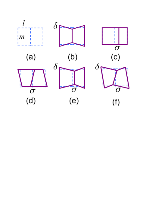
Figure 3: (Color online)Schematic illustration of the dimerization patterns including (a) original lattice, (b) transverse, (c) columnar, (d) staggered, (e) vertical saw-tooth, and (f) inclined saw-tooth. $m$ and $l$ are the lengths of transverse and longitudinal directions, respectively. $\delta$ and $\sigma$ denote the static deformations along transverse and longitudinal directions, respectively.

All five uniform dimerization patterns ,including three simple dimerization patterns and two hybrid ones, are presumed for manovalent case, which is illustrated by a deformed two-square section of the ladder in Fig. 3. The undimerized lattice is present in Fig. 3(a). The first simple case is the rung dimerization (Fig. 3(b)) which possesses lattice deformation only along the transverse direction. Along the longitudinal direction there are two different dimerization patterns: the columnar dimerization (Fig. 3(c)) and the staggered dimerization (Fig. 3(d)), which correspond to same or different Peierls phases in the $a-$ and the $b-$ chain. Last two hybrid dimerization patterns, the vertical saw-tooth (Fig. 3(e)) and the inclined saw-tooth (Fig. 3(f)), are regarded as that the system is transversely and longitudinally dimerized simultaneously, which possess either columnar dimerization or staggered dimerization along longitudinal direction.

II.2 Band spectral structures of the Möbius ladder

Since the Fourier transformation is no longer valid when the boundary is not periodic, we introduce a new operator-value vectors $\mathbf{B}_{j}=U_{j}\mathbf{A}_{j},$ where the site-dependent unitary transformation Zhao is defined as

$$U_{j}=\frac{1}{\sqrt{2}}\left[\begin{array}[]{cc}\exp(-i\theta jl)&-\exp(-i\theta jl)\\ 1&1\end{array}\right],$$ (8)

where $\theta=\pi/\left(Nl\right)$ is half of the momentum quanta. Through this transformation, the period boundary condition $\mathbf{B}_{j+N}=\mathbf{B}_{j}$ is retrieved for the new operator-value vectors. In the new representation, the Hamiltonian

$$H_{e}=\sum_{j=0}^{N-1}\mathbf{B}_{j}^{{\dagger}}\mathbf{M}_{j}^{\prime}\mathbf{B}_{j}-\sum_{j=0}^{N-1}\mathbf{J}_{j}^{\prime}\mathbf{B}_{j}^{{\dagger}}\mathbf{B}_{j+1}+h.c.$$ (9)

is unitarily transformed from Eq. (1), where the new transition matrices

$$\mathbf{M}_{j}^{\prime}=U_{j}\mathbf{M}_{j}U_{j}^{{\dagger}}=\left[\begin{array}[]{cc}G_{j}&\varepsilon_{j}\exp(-i\theta jl)\\ \varepsilon_{j}\exp(i\theta jl)&-G_{j}\end{array}\right]$$ (10)

and

$$\mathbf{J}_{j}^{\prime}=U_{j}\mathbf{J}_{j}U_{j+1}^{{\dagger}}=\left[\begin{array}[]{cc}J_{j}^{\mathrm{a}}\exp(i\theta l)&0\\ 0&J_{j}^{\mathrm{b}}\end{array}\right]$$ (11)

differ from the original ones. Such difference is considered as the global effect induced by the Möbius boundary condition, where an induced gauge field takes responsibility for the cutoff of the transmission spectrum and a stark shift occurs in the energy spectrum Zhao . However, this two effects actually are not significant when we only consider electrons filling in the energy bands for static dimerization with very large site number.

To obtain the static lattice deformations, it is necessary to minimize the total energy $E=E_{\mathrm{e}}+E_{\mathrm{p}}$ versus the lattice deformation. Here, based on Born-Oppenheimer approximation, the total energy including the electron part $E_{\mathrm{e}}$ and the phonon part $E_{\mathrm{p}}$ is obtained by diagonalizing the electron Hamiltonian Eq. (9) and the phonon Hamiltonian Eq. (7), respectively.

We take the staggered dimeriation of the Möbius ladder as an example. Let the $m$ and $l$ be the lattice constants along the transverse and the longitudinal directions, respectively, and we can define the static uniform deformations $u_{j}=\left(-1\right)^{j}\delta$ and $v_{j}=\left(-1\right)^{j}\sigma$. Because the lattice deformation changes the coupling strength and the hopping strength from $G_{0}$ and $J_{0}$ to $G_{0}+\beta(m_{j}^{\mathrm{a}}-m_{j}^{\mathrm{b}})$ and $J_{0}+\alpha(l_{j}-l_{j+1}),$ where $\alpha$ and $\beta$ are the rate of the changes of the longitudinal and the transverse hopping. For the staggered dimeriation, the longitudinal lattice deformation is $l_{j}=l+(-1)^{i+j}\sigma$ and the transverse lattice deformation is

$$m_{j}^{\mathrm{a}}-m_{j}^{\mathrm{b}}=\sqrt{m^{2}+(2\sigma)^{2}}-m\approx 2\sigma^{2}/m.$$ (12)

Therefore, with the modified coupling strength $G_{j}\equiv G_{0}^{\prime}=G_{0}+2\beta\sigma^{2}/m$ and hopping strength $J_{j}^{\mathrm{a}}=J_{0}+\Delta J\left(-1\right)^{j}$ for $a$-chain and $J_{j}^{\mathrm{b}}=J_{0}+\Delta J\left(-1\right)^{j+1}$ for $b$-chain with $\Delta J=2\alpha\sigma$, four separate energy bands of the electrons can be obtained by diagonalizing the Hamiltonian Eq. (9) in the momentum space as

$$\varepsilon_{j}(k) = \left(-1\right)^{j}\sqrt{\mu(\sigma)+(-1)^{\left\lfloor\frac{j}{2}\right\rfloor}\nu(\sigma)},$$ (13a)

$$\mu(\sigma) = G_{\mathrm{m}}^{2}+\Delta J^{2}+4J_{0}^{2}\cos^{2}\left(kl+\frac{\pi}{N}\right),$$ (13b)

$$\nu(\sigma) = 2\sqrt{G_{0}^{\prime 2}\Delta J^{2}+4J_{0}^{2}G_{\mathrm{m}}^{2}\cos^{2}\left(kl+\frac{\pi}{N}\right)}$$ (13c)

for $$j=1,2,3,4, \left\lfloor\frac{j}{2}\right\rfloor j/2.$$ where , and represents the integer part of of

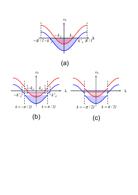
Figure 4: (Color online) Schematic spectra of ladders (a) without dimerization (a) and (b),(c) with staggered dimerization. In (b), four gaps are opened up at Fermi momentum $k_{f}$, $k_{f}^{\prime}$ and $k=\pm\pi/2l$, while in (c) two gaps up at Fermi momentum disappear when the hopping strength $J_{0}$ is sufficiently small. The shadow regions represent the electron occupation in the energy bands.

It follows the energy band diagram (Fig. 4(b)) that when the hopping strength $J_{0}$ is sufficiently large, the deformation opens four gaps in the original two overlapped bands. The two gaps at $k=\pm\pi/2l$ are usual ones because they only arise from the longitudinal deformation for $a$- and $b$-chain, respectively. The other two gaps approximately locating at Fermi momentum $k_{f}=\pm\arccos(G_{\mathrm{m}}/2J_{0})/l$ in the upper band and $k_{f}^{\prime}=\pi/l-k_{f}$ in the lower band basically arise from the coupling between the $k-$ states in $a-$chain and the $k-\pi/l-$states in $b$-chain with strength $\alpha\sigma G_{0}^{\prime}/2J_{0}$ approximately. It is essential to indicate that when the the hopping strength $J_{0}$ is sufficiently small, there are no gaps opened up at Fermi surface even there exists the coupling between the $k$-states in $a$-chain and the $k-\pi/l$-states in $b$-chain (Fig. 4(c)). Thus no Peierls transitions occur.

To compare with the result of the Möbius ladder, we also consider the dimerization in a generic ladder shown in Fig. 1(b). Here, the Fourier transformation is applied to diagonalize the electron Hamiltonian without introducing site-dependent unitary transformation. The staggered dimerization is still taken as an example for the generic ladder, which also possesses four separated energy bands

$$\varepsilon_{j}^{\prime}(k) = \left(-1\right)^{j}\sqrt{\mu^{\prime}(\sigma)+(-1)^{\left\lfloor\frac{j}{2}\right\rfloor}\nu^{\prime}(\sigma)},$$ (14a)

$$\mu^{\prime}(\sigma) = G_{m}^{2}+\Delta J^{2}+4J_{0}^{2}\cos^{2}\left(kl\right),$$ (14b)

$$\nu^{\prime}(\sigma) = 2\sqrt{\varepsilon_{0}^{2}\Delta J^{2}+4J_{0}^{2}G_{m}^{2}\cos^{2}\left(kl\right)},$$ (14c)

which also follows the energy band diagram Fig. 4(b) and Fig. 4(c). However, the gaps opened up at Fermi surface are different from the ones of Möbius case, which results in different energy of each dimerization patterns of generic ladder from the ones of Möbius case and thus the different phase diagrams.

II.3 Phase diagram of the Möbius ladder and the generic ladder

Now we focus on the case that the gaps opened up at Fermi surface may decrease the energy of the electrons by $\Delta E_{\mathrm{e}}=E(\delta)-E(0),$ where

$$E(\delta)=\sum_{i=1,3}\int\varepsilon_{j}(k)dk$$ (15)

and $E(0)$ is the energy without dimerization. The lattice deformation also increases the energy of phonons by

$$\Delta E_{p}=4K_{l}N\sigma^{2}+2K_{t}N\frac{\sigma^{4}}{m^{2}}.$$ (16)

The total energy shift $\Delta E=\Delta E_{e}+\Delta E_{p}$ versus lattice deformation $\sigma$ is plotted in Fig. 5. There is a minimum of $\Delta E$ at $\sigma=\sigma_{s}\left(K_{l},K_{t}\right)$, which corresponds to the stable configuration of the system. Obviously, as the order parameter of the staggered Peierls phase transition in Möbius ladder, $\sigma_{s}\left(K_{l},K_{t}\right)=0$ means the lattice is not deformed corresponding to the original metal phase, while $\sigma_{s}\left(K_{l},K_{t}\right)\neq 0$ means the lattice is spontaneously modulated to form an insulator phase. In this sense, when all the possible $K_{t}$ and $K_{l}$ are chosen to determine respective stable configurations, we obtain the phase diagram of the staggered dimerization in the Möbius ladder.

The above calculation is carried out for the staggered case. Repeating it for all deformations (Fig. 2) gives the total Peierls phase diagram for the Möbius boundary condition (Fig.  5(a)). Here, the parameters are chosen as $G_{0}=15\varepsilon_{0},J_{0}=10\varepsilon_{0},\alpha=\beta=\varepsilon_{0}/m,$ and $l=m.$

With these parameters, only three dimerization patterns survive, which are the rung, the staggered, and the inclined saw-toothed dimerization patterns (all are denoted by capital letters "R", "S", and "I" in Fig. 5(a)). The three Peierls phases occur at different regions at $K_{l}$ and $K_{t}$. The rung dimerization occurs when $K_{l}\gg K_{t},$ the staggered dimerization occurs when $K_{l}\ll K_{t},$ and the inclined saw-toothed dimerization occurs when $K_{l}\approx K_{t}$ is sufficiently small. When $K_{l}\approx K_{t}$ is sufficiently large, there is no dimerization emerging in the Möbius ladder.

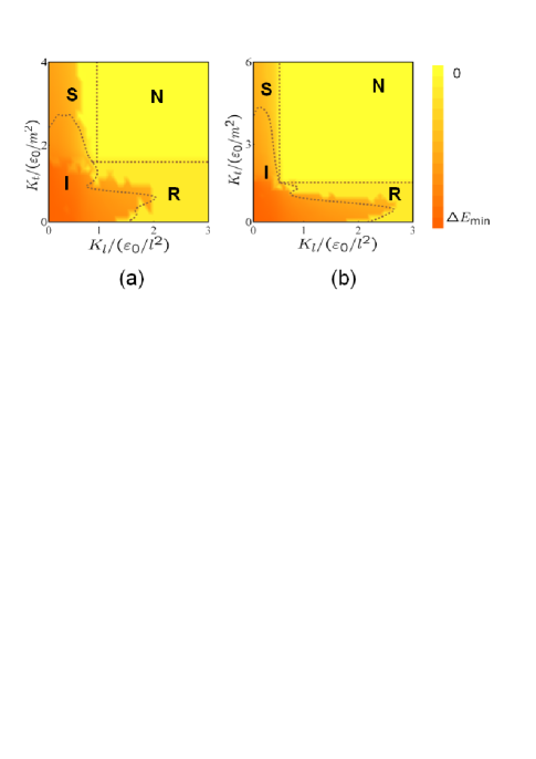
Figure 5: (Color online) The phase diagrams of the ladder system with (a) the generic and (b) the Möbius boundary conditions, which are plotted versus $\left(K_{l},K_{t}\right)$ in (a) and (b), respectively. The parameters are chosen as $G_{0}=15\varepsilon_{0}$, $J_{0}=10\varepsilon_{0}$, $\alpha=\beta=\varepsilon_{0}/m$, and $l=m$.The distribution of the total energy $\Delta E$ versus $\left(K_{l},K_{t}\right)$ determines the boundaries of the phases, which are plotted as dashed lines. Here S, I, R, and N represent the staggered, the inclined saw-tooth, rung and no dimerization, respectively.

With the same procedure, by minimizing $\Delta E$ of the generic ladder, we obtain the total Peierls phase diagram for the generic boundary condition (Fig. 5(b)). Notice here that the energy bands completely filled with electrons become $\varepsilon_{j}^{\prime}(k)$ $(j=1,3)$ in Eq. (14a).

With the same parameters of the Möbius case, the basic properties of the Peierls phases of generic ladder is similar to the one of Möbius case. However, the region of the staggered dimerization pattern under the Möbius boundary condition shrinks comparing with the generic one. This fact means that the metal phase is preferable for a Möbius ladder system. Therefore, the above phase diagrams show that the conducting properties can be dramatically changed in when the topology of the ladder is switched. Because the inclined saw-toothed phase contains the staggered dimerization along longitudinal direction, it is changed the same way as the staggered one. The Peierls phase for rung dimerization is exactly the same whatever the boundary condition is. Although the columnar and the vertical saw-toothed dimerization do not appear in the current phase diagrams in Fig. 5, their corresponding Peierls phases are the same for different boundary conditions of the ladder system when $G_{0}\ll\varepsilon_{0}$. Therefore, to further consider the topological effect on conducting properties, only the staggered dimerization pattern is taken into account and the existence of the localized states will be revisited for our Q1D system.

III Continuum Model and Solitonary Solutions

III.1 localized states in the Möbius ladder

We adapt the continuous field approach by regarding the Möbius ladder as a one-dimensional system with long range hopping (Fig. 1(c)). The detailed derivation of the continuum model from the lattice Hamiltonian Eq. (1) and (7) is presented in App. A. Without loss of the generality, we focus on the special case with $\varepsilon_{0}=0.$ For a continuous field approach, it is crucial to introduce an order parameter

$$\Delta(x)=-4\alpha\phi(x),$$ (17)

where $\phi(x)$ is the continuous limit of $\phi_{j}=\left(-1\right)^{j}u_{j}.$

The Hamiltonian of the continuum model $H=H_{\mathrm{e}}+H_{\mathrm{p}}$ contains the the phonon part

$$H_{\mathrm{p}} = \int_{-L}^{L}dx\left\{\frac{K_{\mathrm{l}}}{8\alpha^{2}l}\Delta^{2}(x)+\frac{M}{32\alpha^{2}l}\overset{\cdot}{\Delta^{2}}(x)\right.+$$ (18)

$$\left.\frac{K_{\mathrm{t}}}{4^{6}m^{2}\alpha^{4}l}\left[\Delta(x+L)-\Delta(x)\right]^{4}\right\}$$

and the electron part

$$H_{\mathrm{e}}=\int_{-L}^{0}dx\Phi(x)\mathscr{H}_{\mathrm{m}}\Phi(x),$$ (19)

where $M$ is the mass of the particle and $L=Nl$ is the length of the $a$-chain ($b$-chain), which approaches infinity at the end of the calculation. Here, the subindex $\mathrm{m}$ stands for the Möbius ladder. In the electron part, the hopping electron could be described with a 4-component spinor $\Phi(x)=\left[\begin{array}[]{cccc}\phi_{1}(x)&\phi_{2}(x)&\phi_{3}(x)&\phi_{4}(x)\end{array}\right]^{\mathrm{T}}.$ Physically, $\phi_{1}(x)$($\phi_{3}(x)$) and $\phi_{2}(x)$($\phi_{4}(x)$) respectively represent the left-traveling wave and right-traveling wave in $a$-chain ($b$-chain). In this spinor representation, the Hamiltonian density is expressed by Pauli matrices $\sigma_{x},$ $\sigma_{y},$ $\sigma_{z}$ as

$$\mathscr{H}_{\mathrm{m}}=\left[\begin{array}[]{cc}iv_{\mathrm{f}}\sigma_{z}\partial_{x}+\Delta(x)\sigma_{x}&G\left(x\right)\\ G\left(x\right)&iv_{\mathrm{f}}\sigma_{z}\partial_{x}+\Delta(x+L)\sigma_{x}\end{array}\right]$$ (20)

where $v_{\mathrm{f}}=2lJ_{0},$ $\sigma_{z},\sigma_{x}$ are Pauli matrices, and

$$G\left(x\right)=G_{0}+\frac{\beta}{32m\alpha^{2}}\left[\Delta(x)-\Delta(x+L)\right]^{2}$$ (21)

is effective coupling between the $a$-chain and $b$-chain.

To reflect the Möbius boundary condition in our Q1D model (Fig. 1(c)), we take the period $2L$ for boundary conditions

$$\Phi\left(x+2L\right)=\Phi\left(x\right)$$ (22)

rather than $L$ for the generic case. With this boundary condition, we solve the Bogoliubov-de Gennes (BdG) equation

$$\mathscr{H}_{\mathrm{m}}\Phi_{i}\left(x\right)=\varepsilon_{i}\Phi_{i}\left(x\right),$$ (23)

where $i$ represents the $i$-th energy band of the spectrum and $\Phi_{i}\left(x\right)=[\phi_{1}^{i}\left(x\right),\phi_{2}^{i}\left(x\right),\phi_{3}^{i}\left(x\right),\phi_{4}^{i}\left(x\right)]^{\mathrm{T}}$. At zero temperature, the order parameter $\Delta\left(x\right)$ satisfies the self-consistent equations

$$\frac{K_{\mathrm{l}}}{4\alpha^{2}l}\Delta(x)-\frac{K_{\mathrm{t}}}{4^{5}m^{2}\alpha^{4}l}(\Delta(x+L)-\Delta(x))^{3}$$ (26)

$$= \left\{\begin{array}[]{c}\sum_{i}2\mathbf{Re}\left[\phi_{1}^{i,\ast}\left(x\right)\phi_{2}^{i}\left(x\right)\right],\text{for }x\leq 0,\\ \sum_{i}2\mathbf{Re}\left[\phi_{3}^{i,\ast}\left(x\right)\phi_{4}^{i}\left(x\right)\right],\text{for }x>0,\end{array}\right.$$

which is obtained by the functional variation of

$$E\left(\Delta\left(x\right)\right)=\sum_{i}\varepsilon_{i}+H_{\mathrm{p}}$$ (27)

with respect to $\delta\Delta\left(x\right)$ and $\delta\Delta\left(x+L\right).$ The sum is over the energy levels below the Fermi surface. In principle, the eigenenergies $\varepsilon_{i},$ the eigenfunctions $\Phi_{i}\left(x\right)$ and the order parameters $\Delta(x)$ and $\Delta\left(x+L\right)$ can be completely determined by the BdG equation in Eq. (23) and the self-consistent equation in in Eq. (26).

After introducing new 4-component spinor $\Psi_{i}(x)=\left[\begin{array}[]{cccc}\varphi_{1}^{i}(x)&\varphi_{2}^{i}(x)&\varphi_{3}^{i}(x)&\varphi_{4}^{i}(x)\end{array}\right]^{\mathrm{T}}$ by $\Psi_{i}(x)=U\Phi_{i}\left(x\right)$, where the unitary matrix is defined as

$$U=\frac{1}{\sqrt{2}}\left[\begin{array}[]{cccc}1&i&0&0\\ 1&-i&0&0\\ 0&0&1&i\\ 0&0&1&-i\end{array}\right],$$ (28)

the BdG equation in Eq. (23) can be simplified as

$$\mathscr{H}_{\mathrm{m}}^{\prime}\Psi_{i}(x)=\varepsilon_{i}\Phi_{i}\left(x\right)$$ (29)

with new Hamiltonian density

$$\mathscr{H}_{\mathrm{m}}^{\prime}=\left[\begin{array}[]{cc}iv_{\mathrm{f}}\sigma_{x}\partial_{x}-\Delta(x)\sigma_{y}&G_{0}\\ G_{0}&iv_{\mathrm{f}}\sigma_{x}\partial_{x}-\Delta(x+L)\sigma_{y}\end{array}\right].$$ (30)

As we shown as follows, some solutions of the above BdG equation can exist as localized states. In the following, we only consider the case $K_{l}\ll K_{t}$. In this case, three dimerization patterns of rung (Fig. 3(b)), vertical-saw tooth (Fig. 3(e)) and inclined saw-tooth (Fig. 3(f)) occur rarely. Thus we only need to compare the energy of staggered dimerization with columnar one. Here, we revisit Möbius ladder system with the staggered dimerization characterized by

$$\Delta\left(x\right)=-\Delta\left(x+L\right).$$ (31)

In this phase, the order parameters in $a$-chain and $b$-chains are opposite and display a Peierls phases domain wall when the site number $N$ is even. We also notice that the columnar dimerization to be compared is characterized by

$$\Delta\left(x\right)=\Delta\left(x+L\right).$$ (32)

For the staggered case, we assume a kink deformation as the form

$$\Delta\left(x\right)=\Delta\tanh(x/\xi)$$ (33)

with $\xi=v_{\mathrm{f}}/\Delta$, which is so small that the effective coupling between the $a$-chain and $b$-chain $G\left(x\right)\approx G_{0}.$

To solve the new BdG equation, some symmetries of the Hamiltonian density can be used to simplify the calculation. The Hamiltonian density actually possesses the discrete symmetry

$$W^{{\dagger}}\mathscr{H}_{\mathrm{m}}^{\prime}W=\mathscr{H}_{\mathrm{m}}^{\prime}$$ (34)

with an anti-diagonal matrix

$$W=W^{{\dagger}}=\left[\begin{array}[]{cccc}0&0&0&1\\ 0&0&1&0\\ 0&1&0&0\\ 1&0&0&0\end{array}\right]$$ (35)

denoting the mirror reflection transformation. This symmetry guarantees that if $\Psi_{i}(x)$ is an eigen function of $\mathscr{H}_{\mathrm{m}}^{\prime}$ with eigenenergy $\varepsilon_{i}$, the $W^{{\dagger}}\Psi_{i}(x)$ is also the eigen function of $\mathscr{H}_{\mathrm{m}}^{\prime}$ with the same eigenenergy $\varepsilon_{i}.$ Obviously, the eigenvalues of matrix W are $\pm 1$. Together with the translational symmetry characterized by momentum quantum numbers, the total Hilbert space can be spanned by these bases. Therefore, the eigen function $\Psi_{i}(x)$ either has the form

$$\Psi_{i}(x)=W\Psi_{i}(x)$$ (36)

or

$$\Psi_{i}(x)=-W\Psi_{i}(x).$$ (37)

In this sense, as the solutions of the BdG equation with energy $\varepsilon_{\mathrm{s}}=0$, two degenerate solitonary states can be found as one with non-vanishing components

$$\varphi_{2}^{\mathrm{s}}\left(x\right)=\varphi_{3}^{\mathrm{s}}\left(x\right)=F_{+}^{\mathrm{s}}(x),$$ (38)

and another with non-vanishing components

$$\varphi_{2}^{\mathrm{s}}\left(x\right)=-\varphi_{3}^{\mathrm{s}}\left(x\right)=F_{-}^{\mathrm{s}}(x)$$ (39)

for

$$F_{\pm}^{\mathrm{s}}\left(x\right)=\sqrt{\frac{1}{2\xi}}\exp\left(\pm i\frac{G_{0}}{v_{\mathrm{f}}}x\right)\text{sech}\left(\frac{x}{\xi}\right),$$ (40)

where the subindex $\mathrm{s}$ denotes solitonary solutions. These solitonary states are the localized states located at the midgap. Since there is no such solitonary state in the generic ladder, the existence of the solitons is absolutely topological effect.

We note that the another two bands

$$\varepsilon_{\mathrm{v}}^{\pm}=-\sqrt{\left(v_{\mathrm{f}}k\pm G_{0}\right)^{2}+\Delta}$$ (41)

(illustrated in Fig. 6(a) as two overlapped shadowed domains) fully occupied by the electrons correspond to eigen functions

$$\varphi_{1}^{\mathrm{v},\pm}\left(x\right) = \pm\varphi_{4}^{\mathrm{v},\pm}\left(x\right)=\frac{i}{2\sqrt{L}}e^{-ikx},$$ (42a)

$$\varphi_{2}^{\mathrm{v},\pm}\left(x\right) = \pm\varphi_{3}^{\mathrm{v},\pm}\left(x\right)=\frac{1}{2\sqrt{L}}F_{\pm}^{\mathrm{v}}(x)e^{-ikx},$$ (42b)

where

$$F_{\pm}^{\mathrm{v}}(x)=\frac{\Delta}{\varepsilon_{\mathrm{v}}^{\pm}}\left[\tanh\frac{\Delta x}{v_{\mathrm{f}}}+i\frac{\left(v_{\mathrm{f}}k\pm G_{0}\right)}{\Delta}\right]$$ (43)

represents a deviation from a plane wave in the kink order. Here, the subindex $\mathrm{v}$ stands for the valence bands below the Fermi surface.

Then, it follows from the self-consistent equations Eq. (26) that

$$\frac{K_{l}}{4\alpha^{2}l}+\frac{2K_{t}}{4^{4}m^{2}\alpha^{4}l}\Delta^{2}\tanh^{2}(x/\xi)$$ (44)

$$= \frac{1}{2\pi}\int_{-k_{\mathrm{f}}}^{k_{\mathrm{f}}}\frac{dk}{\sqrt{v_{\mathrm{f}}^{2}k_{\mathrm{f}}^{2}+\Delta^{2}}}.$$

Usually, the solitons are localized around the original point with the width $\xi$ of several lattice constants, which is much smaller than the total length of the ladder system. For most sites far away from the original point as $|x|\gg|\xi|$, we assume $\tanh^{2}(x/\xi)\approx 1$. Since the second term is small comparing with the first term at the left side of the above equation, we obtain approximate order parameter

$$\Delta\approx\Delta_{0}\exp(-B\Delta_{0}^{2}),$$ (45)

where $\Delta_{0}=W\exp(-A)$ is the order parameter for one dimensional uniformly dimerized system, $W=2v_{\mathrm{f}}k_{\mathrm{f}}$, $A=v_{\mathrm{f}}\pi K_{l}/8\alpha^{2}l$, and $B=v_{\mathrm{f}}\pi K_{t}/2^{7}m^{2}\alpha^{4}l$ with $k_{\mathrm{f}}$ is the Fermi momentum.

Moreover, we can further prove that the above solitonary states are the ground states. To this end we calculate the total energy of the electron-phonon system $E_{\mathrm{T}}^{\mathrm{S}}$ according to the phase shift PT2 of the eigenstates. The phase shifts are determined by the eigenstates of the band electrons  when $x$ tends to $\pm\infty$ as

$$\lim_{x\rightarrow\pm\infty}F_{\pm}^{\mathrm{v}}(x) = \frac{\Delta}{\varepsilon_{\mathrm{v}}^{\pm}}\left[\pm 1+i\frac{\left(v_{\mathrm{f}}k\pm G_{0}\right)}{\Delta}\right]$$ (46)

$$\propto \exp(i\theta_{\pm\infty}^{\pm}\left(k\right)),$$

which reads

$$\theta_{+\infty}^{\pm}\left(k\right) = \arctan\left(\frac{v_{\mathrm{f}}k\pm G_{0}}{\Delta}\right),$$ (47a)

$$\theta_{-\infty}^{\pm}\left(k\right) = -\arctan\left(\frac{v_{\mathrm{f}}k\pm G_{0}}{\Delta}\right)-\pi.$$ (47b)

Therefore, the total phase shift of the eigenstates is defined by their difference as

$$\theta^{\pm}\left(k\right)=\theta_{+\infty}^{\pm}\left(k\right)-\theta_{-\infty}^{\pm}\left(k\right)=\pi+2\arctan\left(\frac{v_{\mathrm{f}}k\pm G_{0}}{\Delta}\right).$$ (48)

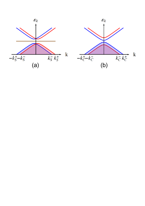
Figure 6: (color online) Schematics of the energy spectra of the valence bands under (a) staggered and (b) columnar dimerizations, where $k_{\mathrm{S}}^{\pm}=k_{\mathrm{f}}\mp G_{0}/v_{\mathrm{f}}$ and $k_{\mathrm{C}}^{\pm}=\sqrt{G_{0}^{2}+v_{\mathrm{f}}^{2}k_{\mathrm{f}}^{2}\pm 2G_{0}\sqrt{v_{\mathrm{f}}^{2}k_{\mathrm{f}}^{2}+\Delta^{2}}}/v_{\mathrm{f}}.$ The shadow regions represent the electron occupation in the energy bands, and the brown straight line represents the solitonary states.

A straightforward algebra explicitly gives PT2

$$E_{\mathrm{T}}^{\mathrm{S}}=E_{\mathrm{T}}^{\mathrm{C}}+\frac{4\Delta}{\pi}-\frac{G_{0}^{2}}{v_{\mathrm{f}}k_{\mathrm{f}}}+\delta(K_{\mathrm{t}}),$$ (49)

where $E_{\mathrm{T}}^{\mathrm{C}}$ is the total energy for the columnar dimerization (Fig. 3(c)), and $\delta(K_{\mathrm{t}})=13K_{\mathrm{t}}\Delta^{3}v_{\mathrm{f}}/(3\times 4^{4}m^{2}\alpha^{4}l)$ results from the coupling between the $a$- and $b$-chain. The second term in $E_{\mathrm{T}}^{\mathrm{S}}$ is usual energy increment due to the existence of solitonary states. The third term in $E_{\mathrm{T}}^{\mathrm{S}}$ results from the difference in the total energies in two filling ways. One corresponds to the staggered dimerization (Fig. 6(a)) with two lower bands $-\sqrt{\left(v_{\mathrm{f}}k\pm G_{0}\right)^{2}+\Delta^{2}}$ occupied by electrons, while the other corresponds to columnar one (Fig. 6(b)) with two lower bands $\pm G_{0}-\sqrt{\left(v_{\mathrm{f}}k\right)^{2}+\Delta^{2}}$ occupied. For the latter the energy of electrons increases because a part of electrons are forced to occupy higher energy levels. If $G_{0}$ is so large that $\delta E=E_{\mathrm{T}}^{\mathrm{S}}-E_{\mathrm{T}}^{\mathrm{C}}$ is negative, the ground state of the Möbius ladder system corresponds to the staggered dimerization rather than the columnar one. In this case the solitonary states are localized states as the ground state.

III.2 Comparison with the generic ladder

It is a complete topological effect that the ground state is localized. To demonstrate this, the continuum model for the generic ladder $H^{\prime}=H_{\mathrm{e}}^{\prime}+H_{\mathrm{p}}^{\prime}$ is presented to compare with the Möbius case. Here, the phonon part is

$$H_{\mathrm{p}}^{\prime} = \sum_{c=a,b}\int_{-\infty}^{\infty}dx\left\{\frac{K_{\mathrm{l}}}{8\alpha^{2}l}\Delta_{\mathrm{c}}^{2}(x)+\frac{M}{32\alpha^{2}l}\overset{\cdot}{\Delta_{\mathrm{c}}^{2}}(x)\right\}+$$ (50)

$$\int_{-\infty}^{\infty}dx\frac{K_{\mathrm{t}}}{4^{6}m^{2}\alpha^{4}l}\left[\Delta_{\mathrm{a}}(x)-\Delta_{\mathrm{b}}(x)\right]^{4}$$

and the electron part is

$$H_{\mathrm{e}}^{\prime}=\int_{-\infty}^{\infty}dx\Phi^{\prime}(x)\mathscr{H}_{\mathrm{g}}\Phi^{\prime}(x),$$ (51)

where the 4-component spinor $\Phi_{i}^{g}\left(x\right)$ has the same physical meaning as the one in the Möbius case, and the Hamiltonian density reads

$$\mathscr{H}_{\mathrm{g}}=\left[\begin{array}[]{cc}iv_{\mathrm{f}}\sigma_{z}\partial_{x}+\Delta_{\mathrm{a}}(x)\sigma_{x}&G_{0}^{\prime}\\ G_{0}^{\prime}&iv_{\mathrm{f}}\sigma_{z}\partial_{x}+\Delta_{\mathrm{b}}(x)\sigma_{x}\end{array}\right]$$ (52)

where

$$G\left(x\right)=G_{0}+\frac{\beta}{32m\alpha^{2}}\left[\Delta_{\mathrm{a}}(x)-\Delta_{\mathrm{b}}(x)\right]^{2}$$ (53)

is effective coupling between the $a$-chain and $b$-chain. It is noticed that the order parameters here are no longer unified in one chain, and are defined as $\Delta_{\mathrm{a}}(x)$ and $\Delta_{\mathrm{b}}\left(x\right)$ for $a$-chain and $b$-chain, respectively. Additionally, the boundary condition for the generic ladder is $\Phi^{\prime}\left(x+L\right)=\Phi^{\prime}\left(x\right)$ with period $L.$ We will show that because of the trivial topology of the generic ladder, there is no solitonary solution for the dimerization of the generic ladder.

At zero temperature, the order parameter $\Delta\left(x\right)$ satisfies the self-consistent equations

$$\frac{K_{\mathrm{l}}}{4\alpha^{2}l}\Delta_{a}(x)+\frac{K_{\mathrm{t}}}{4^{5}m^{2}\alpha^{4}l}(\Delta_{\mathrm{a}}(x)-\Delta_{\mathrm{b}}(x))^{3}$$

$$= \sum_{i}2\mathbf{Re}\left[\left(\phi_{1}^{i,\prime}\left(x\right)\right)^{\ast}\phi_{2}^{i,\prime}\left(x\right)\right],$$

$$\frac{K_{\mathrm{l}}}{4\alpha^{2}l}\Delta_{b}(x)-\frac{K_{\mathrm{t}}}{4^{5}m^{2}\alpha^{4}l}(\Delta_{\mathrm{a}}(x)-\Delta_{\mathrm{b}}(x))^{3}$$

$$= \sum_{i}2\mathbf{Re}\left[\left(\phi_{3}^{i,\prime}\left(x\right)\right)^{\ast}\phi_{4}^{i,\prime}\left(x\right)\right],$$ (54b)

respectively, which are obtained by the functional variation of

$$E\left(\Delta\left(x\right)\right)=\sum_{i}\varepsilon_{i}+H_{\mathrm{p}}$$ (55)

with respect to $\delta\Delta_{\mathrm{a}}\left(x\right)$ and $\delta\Delta_{\mathrm{b}}\left(x\right).$ The sum is over the energy levels below the Fermi surface. For the staggered case, we assume a kink deformation $\Delta_{\mathrm{a}}\left(x\right)=-\Delta_{\mathrm{b}}\left(x\right)=\Delta.$

After applying the same transformation, the BdG equation of the staggered dimerized generic ladder is

$$\mathscr{H}_{\mathrm{g}}^{\prime}\Psi_{i}^{\prime}(x)=\varepsilon_{i}^{\prime}\Psi_{i}^{\prime}(x)$$ (56)

with new Hamiltonian density

$$\mathscr{H}_{\mathrm{g}}^{\prime}=\left[\begin{array}[]{cc}iv_{\mathrm{f}}\sigma_{x}\partial_{x}-\Delta\sigma_{y}&G_{0}^{\prime}\\ G_{0}^{\prime}&iv_{\mathrm{f}}\sigma_{x}\partial_{x}+\Delta\sigma_{y}\end{array}\right],$$ (57)

where $G_{0}^{\prime}=G_{0}+\beta\Delta^{2}/8m\alpha^{2}.$

The exact spectrum solved from the BdG equations contains four energy bands including the lower two bands $\varepsilon_{\mathrm{v}}^{\prime,\pm}=-\sqrt{\left(v_{\mathrm{f}}k\pm G_{0}\right)^{2}+\Delta}$ occupied by the electrons and the higher two bands $\varepsilon_{\mathrm{v}}^{\prime,\pm}=\sqrt{\left(v_{\mathrm{f}}k\pm G_{0}\right)^{2}+\Delta}$ without being occupied. The corresponding eigen function are

$$\varphi_{1,\mathrm{g}}^{\mathrm{v},\pm}\left(x\right) = \pm\varphi_{4,\mathrm{g}}^{\mathrm{v},\pm}\left(x\right)=\mp\frac{1}{2\sqrt{L}}e^{i\left(\frac{G_{0}^{\prime}}{v_{\mathrm{f}}}-k\pm\theta_{k}^{\pm}\right)x},$$ (58a)

$$\varphi_{2,\mathrm{g}}^{\mathrm{v},\pm}\left(x\right) = \pm\varphi_{3,\mathrm{g}}^{\mathrm{v},\pm}\left(x\right)=\frac{1}{2\sqrt{L}}e^{i\left(\frac{G_{0}^{\prime}}{v_{\mathrm{f}}}-k\right)x},$$ (58b)

for the two lower bands and

$$\varphi_{1,\mathrm{g}}^{\mathrm{v},\pm}\left(x\right) = \pm\varphi_{4,\mathrm{g}}^{\mathrm{v},\pm}\left(x\right)=\pm\frac{1}{2\sqrt{L}}e^{i\left(\frac{G_{0}^{\prime}}{v_{\mathrm{f}}}-k\pm\theta_{k}^{\pm}\right)x},$$ (59a)

$$\varphi_{2,\mathrm{g}}^{\mathrm{v},\pm}\left(x\right) = \pm\varphi_{3,\mathrm{g}}^{\mathrm{v},\pm}\left(x\right)=\frac{1}{2\sqrt{L}}e^{i\left(\frac{G_{0}^{\prime}}{v_{\mathrm{f}}}-k\right)x},$$ (59b)

for the two upper bands, respectively. Here, the subindex $\mathrm{g}$ stands for the generic ladder.

There is no solitonary solution existing for the staggered dimerization pattern of the generic ladder. Therefore, the localized states are the complete topological effect.

The Möbius ladder with staggered dimerization actually behaves like a topological insulator. Naturally, the Möbius configuration is $\mathbb{Z}^{2}$ topologically invariant and gapless localized states exist in the gap. Aditionally, the topology of the system can protect the solitonary states from external perturbations. For example, when the soliton propagates along the longitudinal directions without spreading, the energy increment caused by moving soliton with velocity $v_{\mathrm{s}}$ from the time evolution of order parameter $\Delta\left(x,t\right)\equiv\Delta\tanh(x-v_{\mathrm{s}}t)/\xi$ is $\Delta E_{\mathrm{s}}=Mv_{\mathrm{s}}^{2}\Delta^{3}/(24v_{\mathrm{f}}\alpha^{2}l)$, which could be much smaller than the exciting energy $\delta E$. It indicates that the moving solitons can propagate in the Möbius ladder without dispersion and thus is robust to external perturbations.

IV CONCLUSION

We study the topological properties of Peierls transitions in a monovalent Möbius ladder in contrast to the Peierls transitions in a generic ladder. According to lattice deformation along the transverse and longitudinal directions of the ladder configuration, there exist plenty Peierls phases corresponding to various dimerization patterns. The insulator phase resulted from staggered modulation along longitudinal direction behaves as a topological insulator, which is different from mundane band insulator. Actually, this non-trivial insulator originates from the Peierls phases boundary induced by the non-trivial $\mathbb{Z}^{2}$ topological configuration.

Appendix A The Derivation of the Continuum Model

When the site number $N$ is so large that the characteristic wave length of the eigen function is greater than the lattice constant $l$, the continuum field approach is appropriately adapted by regarding the Möbius ladder as a one-dimensional system with long range hopping (Fig.1(c)). We consider the upper chain ($a$-chain) and lower chain ($b$-chain) as the first half and second half of a whole chain with $2N$ sites, which corresponds to the mapping

$$a_{j}\rightarrow A_{j},b_{j}\rightarrow A_{j+N}$$ (60)

with fermionic operators $A_{j}.$ After the mapping, the electron part of the lattice Hamiltonian in Eq. (1) with a fixed deformation configuration $\{u_{j}\}=\{u_{j}^{a},u_{j}^{b}\}$ can be rewritten as

$$H_{\mathrm{e}} = \sum_{j=0}^{N-1}\varepsilon_{0}A_{j}^{\dagger}A_{j}-\sum_{j=0}^{N-1}J_{j}^{\mathrm{a}}\left(A_{j}^{\dagger}A_{j+1}+h.c.\right)$$ (61)

$$-\sum_{j=N}^{2N-1}\varepsilon_{0}A_{j}^{\dagger}A_{j}-\sum_{j=N}^{2N-1}J_{j}^{\mathrm{b}}\left(A_{j}^{\dagger}A_{j+1}+h.c.\right)$$

$$-\sum_{j=0}^{N-1}G_{j}\left(A_{j}^{\dagger}A_{j+N}+A_{j+N}^{\dagger}A_{j}\right),$$

where the modified coupling constants are

$$G_{j} = G_{0}+\beta\frac{\left(u_{j}^{\mathrm{b}}-u_{j}^{\mathrm{a}}\right)^{2}}{2m},$$ (62a)

$$J_{j}^{\mathrm{c}} = J_{0}+\alpha\left(u_{j+1}^{\mathrm{c}}-u_{j}^{\mathrm{c}}\right),\left(\mathrm{c=a,b}\right),$$ (62b)

and indecies $$\mathrm{a,b} a b$$ stand for the original -chain and -chain. The energy of the phonon in Eq. (7) can also be obtained as

$$H_{\mathrm{p}} = \sum_{j=0}^{N-1}\frac{K_{\mathrm{l}}}{2}\left(u_{j+1}^{\mathrm{a}}-u_{j}^{\mathrm{a}}\right)^{2}+\sum_{j=0}^{N-1}\frac{M}{2}\left(\dot{u_{j}^{\mathrm{a}}}\right)^{2}$$ (63)

$$+\sum_{j=N}^{2N-1}\frac{K_{\mathrm{l}}}{2}\left(u_{j+1}^{\mathrm{b}}-u_{j}^{\mathrm{b}}\right)^{2}+\sum_{j=N}^{2N-1}\frac{M}{2}\left(\dot{u_{j}^{\mathrm{b}}}\right)^{2}$$

$$+\sum_{j=0}^{N-1}\frac{K_{\mathrm{t}}}{2}\frac{\left(u_{j}^{\mathrm{b}}-u_{j}^{\mathrm{a}}\right)^{4}}{4m^{2}}.$$

Usually the wavefunction varies greatly from site to site under dimerization, which means the coordinate $j$ is not suitable for the continuous field approach. However, if we introduce the new coordinate

$$x_{j}\rightarrow(2j+\frac{1}{2})l$$ (64)

as the center of the $2j$-th and $\left(2j+1\right)$-th sites, the wavefunction varies slowly and the continuous field approach is valid.

In this sense, the new fermionic field operators

$$\begin{cases}\varphi_{1}\left(x_{j}\right)=\frac{1}{\sqrt{2}}\left(-1\right)^{j}\left(iA_{2j}+A_{2j+1}\right),\\ \varphi_{2}\left(x_{j}\right)=\frac{1}{\sqrt{2}}\left(-1\right)^{j}\left(A_{2j}+iA_{2j+1}\right),\end{cases}$$ (65)

which satisfy the anti-commutate relations

$$\left\{\varphi_{\mathrm{c}}\left(x_{j}\right),\varphi_{\mathrm{d}}^{\dagger}\left(x_{j^{\prime}}\right)\right\}_{+} = \delta_{c,d}\delta_{j,j^{\prime}},(\mathrm{c},\mathrm{d}=1,2),$$ (66a)

$$\left\{\varphi_{\mathrm{c}}\left(x_{j}\right),\varphi_{\mathrm{d}}\left(x_{j^{\prime}}\right)\right\}_{+} = 0,$$ (66b)

corresponds to the slowly varying wavefunctions of the new coordinate $$x_{j}. x_{j}$$ Thus the field operators at can be expanded as

$$\varphi_{\mathrm{c}}\left(x_{j+1}\right)=\varphi_{\mathrm{c}}\left(x_{j}\right)+\left[\frac{\partial\varphi_{\mathrm{c}}\left(x\right)}{\partial x}\right]_{x=x_{j}}2l+\cdots,(\mathrm{c}=1,2).$$ (67)

The dimerization implies the deformations $u_{j}^{\mathrm{c}}=\left(-1\right)^{j}\phi_{j}^{\mathrm{c}}$, which leads the displacement order parameters

$$\Delta^{\mathrm{c}}\left(x_{j}\right) = -4\alpha\phi^{\mathrm{c}}\left(x_{j}\right)$$ (68)

$$= -2\alpha\left(\phi_{2j}^{\mathrm{c}}+\phi_{2j+1}^{\mathrm{c}}\right).$$

As $2N$ is very large, the summation can be substituted with the integral

$$\sum_{j=0}^{2N-1}\rightarrow\int_{-\infty}^{\infty}dx/2l.$$ (69)

as well as the field operators

$$\varphi_{\mathrm{c}}\left(x_{j}\right)\rightarrow\sqrt{2l}\varphi_{\mathrm{c}}\left(x\right).$$ (70)

Obviously, from Eq. (66a) and (66b), the above field operators $\varphi_{\mathrm{c}}\left(x\right)$ satisfy the anti-commutate relations

$$\left\{\varphi_{\mathrm{c}}\left(x\right),\varphi_{\mathrm{d}}^{\dagger}\left(x^{\prime}\right)\right\}_{+} = \delta_{\mathrm{c,d}}\delta\left(x-x^{\prime}\right),(\mathrm{c,d=0,1}),$$ (71a)

$$\left\{\varphi_{\mathrm{c}}\left(x\right),\varphi_{\mathrm{d}}\left(x^{\prime}\right)\right\}_{+} = 0.$$ (71b)

Finally, substituting the Eq. (67)-(70) into Eq. (61) and (63), the continuum model of the system is obtained as

$$H = H_{\mathrm{e}}+H_{\mathrm{p}},$$ (72a)

$$H_{\mathrm{p}} = \int_{-L}^{L}dx\left\{\frac{K_{\mathrm{l}}}{8\alpha^{2}l}\Delta^{2}(x)+\frac{M}{32\alpha^{2}l}\overset{\cdot}{\Delta^{2}}(x)\right.+$$ (72b)

$$\left.\frac{K_{\mathrm{t}}}{4^{6}m^{2}\alpha^{4}l}\left[\Delta(x+L)-\Delta(x)\right]^{4}\right\},$$

$$H_{\mathrm{e}} = \int_{-L}^{0}dx\Phi(x)\mathscr{H}_{\mathrm{m}}\Phi(x),$$ (72c)

where the Hamiltonian density is

$$\mathscr{H}_{\mathrm{m}}=\left[\begin{array}[]{cc}iv_{\mathrm{f}}\sigma_{z}\partial_{x}+\Delta(x)\sigma_{x}&G\left(x\right)\\ G\left(x\right)&iv_{\mathrm{f}}\sigma_{z}\partial_{x}+\Delta(x+L)\sigma_{x}\end{array}\right],$$ (73)

and we have unified the order parameters with $\Delta(x)=\Delta^{\mathrm{a}}\left(x\right)$ and $\Delta(x+L)=\Delta^{\mathrm{b}}\left(x\right),$ with a 4-component spinor $\Phi(x)=\left[\begin{array}[]{cccc}\phi_{1}(x)&\phi_{2}(x)&\phi_{3}(x)&\phi_{4}(x)\end{array}\right]^{\mathrm{T}}$ and modified coupling constant

$$G\left(x\right)=G_{0}+\beta\frac{\left(\Delta^{\mathrm{b}}\left(x\right)-\Delta^{\mathrm{a}}\left(x\right)\right)^{2}}{32m\alpha^{2}}.$$ (74)

References

- (1) V. Balzani, A. Credi, and M. Venturi, Molecular Devices and Machines: A Journey Into the Nanoworld (Wiley- VCH Verlag GmbH & Co. KGaA, Weinheim, 2003).
- (2) A. Nitzan and M. A. Ratner, Science 300, 1384 (2003).
- (3) K. Burke, R. Car, and R. Gebauer, Phys. Rev. Lett. 94, 146803 (2005).
- (4) C. Zhang, M. H. Du, H. P. Cheng, X. G. Zhang, A. E. Roitberg, and J. L. Krause, Phys. Rev. Lett. 92, 158301 (2004).
- (5) M. J. Comstock, N. Levy, A. Kirakosian, J. Cho, F. Lauterwasser, J. H. Harvey, Phys. Rev. Lett. 99, 038301 (2007).
- (6) E. Heilbronner, Tetrahedron Lett. 29, 1923 (1964).
- (7) D. J. Ballon, Phys. Rev. Lett. 101, 247701 (2008).
- (8) D. M. Walba, R. M. Richards, and R. C. Haltiwanger, J. Am. Chem. Soc. 104, 3219 (1982).
- (9) S. Tanda, T. Tsuneta, Y. Okajima, K. Inagaki, K. Yamaya, and N. Hatakenaka, Nature London 417, 397 2002.
- (10) C. Castro, C. M. Isborn, W. L. Karney, M. Mauksch, and P. V. R. Schleyer, Org. Lett. 4, 3431 2002.
- (11) H. S. Rzepa, Chem. Rev. 105, 3697 (2005).
- (12) R. Herges, Chem. Rev. 106, 4820 (2005).
- (13) Nan Zhao, H. Dong, Shuo Yang, and C. P. Sun, Phys. Rev. B 79, 125440 (2009).
- (14) Z. L. Guo, Z. R. Gong, C. P. Sun, accepted in Phys. Rev. B (2009).
- (15) A. L. Magna and I. Deretzis, Phys. Rev. Lett. 99, 136404 (2007).
- (16) C. Q. Wu, J. X. Li, and D. H. Lee, Phys. Rev. Lett. 99, 038302 (2007).
- (17) W. P. Su, J. R. Schrieffer, and A. J. Heeger, Phys. Rev. Lett. 42, 1698 (1979).
- (18) H. Takayama, Y. R. Lin-Liu, and K. Maki, Phys. Rev. B 21, 2388 (1980).
- (19) X. G. Wen, Phys. Rev. Lett. 64, 2206 (1990).
- (20) X. G. Wen, Phys. Rev. B 41, 12838 (1990).
- (21) S. C. Zhang, Physics. 1, 6 (2008).
- (22) C. L. Kane and E. J. Mele, Phys. Rev. Lett. 95, 146802 (2005).
- (23) C. J. Isham Modern Differential Geometry for Physicists (second version) (World Scientific, Singapore, 1999).