Optimal thermal refrigerator.

Abstract

We study a refrigerator model which consists of two $n$-level systems interacting via a pulsed external field. Each system couples to its own thermal bath at temperatures $T_{h}$ and $T_{c}$, respectively ($\theta\equiv T_{c}/T_{h}<1$). The refrigerator functions in two steps: thermally isolated interaction between the systems driven by the external field and isothermal relaxation back to equilibrium. There is a complementarity between the power of heat transfer from the cold bath and the efficiency: the latter nullifies when the former is maximized and vice versa. A reasonable compromise is achieved by optimizing over the inter-system interaction and intra-system energy levels the product of the heat-power and efficiency. The efficiency is then found to be bounded from below by $\zeta_{\rm CA}=\frac{1}{\sqrt{1-\theta}}-1$ (an analogue of Curzon-Ahlborn efficiency for refrigerators), besides being bound from above by the Carnot efficiency $\zeta_{\rm C}=\frac{1}{1-\theta}-1$. The lower bound is reached in the equilibrium limit $\theta\to 1$, while the Carnot bound is reached (for a finite power and a finite amount of heat transferred per cycle) in the macroscopic limit $\ln n\gg 1$. The efficiency is exactly equal to $\zeta_{\rm CA}$, when the above optimization is constrained by assuming homogeneous energy spectra for both systems.

Thermodynamics studies principal limitations imposed on the performance of thermal machines, be they macroscopic heat engines or refrigerators callen , or small devices in nanophysics q_t and biology venturi . Let us recall three basic definitions applicable to any thermal machine taking as an example a refigerator driven by a source of work: i) heat $Q_{c}$ transferred per cycle of operation from a cold body at temperature $T_{c}$ to a hot body at temperature $T_{h}$ ($T_{h}>T_{c}$). ii) Power, which is $Q_{c}$ divided over the cycle duration $\tau$. iii) Efficiency (or performance coefficient) $\zeta=Q_{c}/W$, which quantifies the useful output $Q_{c}$ over the work $W$ spent by the work-source for making the cycle. The second law imposes the Carnot bound $\zeta\leq\zeta_{\rm C}=T_{c}/(T_{h}-T_{c})$ on the efficiency of refrigeration callen . Within the usual thermodynamics the Carnot bound is reached only for a reversible, i.e., an infinitely slow process, which means it is reached at zero power callen . The practical value of the Carnot bound is frequently questioned on this ground. The drawback of zero power is partially cured within finite-time thermodynamics (FTT), which is still based on the quasi-equilibrium concepts ftt . For heat-engines FTT gives an upper bound $\eta\leq\eta_{\rm CA}\equiv 1-\sqrt{T_{c}/T_{h}}$ (Curzon-Ahlborn, or CA efficiency) for the efficiency $\eta$ at the maximal power of work-extraction ca ; broek . Naturally, $\eta_{\rm CA}$ is smaller than the Carnot upper bound $1-T_{c}/T_{h}$ for heat-engines.

Heat engines have recently been studied within microscopic theories, where one is easily able to go beyond the quasi-equilibrium regime kosloff ; armen ; tu ; izumida_okuda ; udo ; esposito ; jmod ; henrich . For certain classes of heat-engines the CA efficiency is a lower bound for the efficiency at the maximal power of work armen ; tu ; izumida_okuda . This bound is reached at the quasi-equilibrium situation $T_{h}\to T_{c}$ in agreement with the finding of FTT. The result is consistent with other studies udo ; esposito .

The situation with refrigerators at a finite power is less clear, though yan_chen ; velasco ; jimenez ; unified . Here maximizing the power of cooling does not lead to reasonable results, since there is an additional complementarity (not present for heat engines) velasco : when maximizing the power one simultaneously minimizes the efficiency to zero, and vice versa.

We study optimal regimes of finite-power refrigeration via a realistic model, which can be optimized over almost all of its parameters. The model is quantum, but it admits a classical interpretation. The interest in small-scale refrigerators is triggered by the importance of of cooling processes for functioning of small devices and for displaying quantum features of matter q_t ; henrich ; feldman ; segal ; rezek .

Consider two quantum systems ${\rm\bf H}$ and ${\rm\bf C}$ with Hamiltonians $H_{\rm\bf H}$ and $H_{\rm\bf C}$, respectively. Each system has $n$ energy levels. Initially, ${\rm\bf H}$ and ${\rm\bf C}$ do not interact and are in equilibrium at temperatures $T_{h}=1/\beta_{h}>T_{c}=1/\beta_{c}$:

$$\rho={e^{-\beta_{h}H_{\rm\bf H}}}/{{\rm tr}\,[e^{-\beta_{h}H_{\rm\bf H}}]},~{}~{}\sigma={e^{-\beta_{c}H_{\rm\bf C}}}/{{\rm tr}\,[e^{-\beta_{c}H_{\rm\bf C}}]},$$ (1)

where $\rho$ and $\sigma$ are the initial Gibbsian density matrices of ${\rm\bf H}$ and ${\rm\bf C}$, respectively. We write

$$\rho={\rm diag}[r_{n},...,r_{1}],\quad r_{n}\leq...\leq r_{1},$$

$$\sigma={\rm diag}[s_{n},...,s_{1}],\quad s_{n}\leq...\leq s_{1},$$ (2)

$$H_{\rm\bf H}={\rm diag}[\varepsilon_{n},...,\varepsilon_{1}=0\,],\,\,\varepsilon_{n}\geq...\geq\varepsilon_{1},$$

$$H_{\rm\bf C}={\rm diag}[\mu_{n},...,\mu_{1}=0\,],\,\,\mu_{n}\geq...\geq\mu_{1},$$ (3)

where ${\rm diag}[a,..,b]$ is a diagonal matrix with entries $(a,...,b)$, and where without loss of generality we have nullified the lowest energy level of both ${\rm\bf H}$ and ${\rm\bf C}$. Thus the overall initial density matrix is $\Omega_{\rm in}=\rho\otimes\sigma$, and the initial Hamiltonian $H_{\rm\bf H}\otimes 1+1\otimes H_{\rm\bf C}$.

The goal of any refrigerator is to transfer heat from the cooler bath to the hotter one at the expense of consuming work from an external source. The present refrigerator model functions in the following two steps; see Fig. 1.

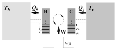
Figure 1: The refrigerator model. Two systems ${\rm\bf H}$ and ${\rm\bf C}$ operate between two baths at temperatures $T_{c}<T_{h}$ and are driven by an external potential $V(t)$. $W$ and $Q_{c}$ and $Q_{h}$ are, respectively, the work put into the overall system and the heats transferred from the cold bath and to the hot bath.

1. ${\rm\bf H}$ and ${\rm\bf C}$ interact with each other and with external sources of work. The overall interaction is described via a time-dependent potential $V(t)$ in the total Hamiltonian $H_{\rm\bf H}\otimes 1+1\otimes H_{\rm\bf C}+V(t)$ of ${\rm\bf H}+{\rm\bf C}$. The interaction process is thermall isolated: $V(t)$ is non-zero only in a short time-window $0\leq t\leq\delta$ and is so large there that the influence of all other couplings [e.g., couplings to the baths] can be neglected [pulsed regime]. Thus the dynamics of ${\rm\bf H}+{\rm\bf C}$ is unitary for $0\leq t\leq\delta$:

$$\Omega_{\rm f}\equiv\Omega(\delta)={\cal U}\,\Omega_{\rm i}\,{\cal U}^{\dagger},\qquad{\cal U}={\cal T}e^{-\frac{i}{\hbar}\int_{0}^{\delta}{\rm d}sV(s)}$$ (4)

where $\Omega_{\rm i}=\Omega(0)=\rho\otimes\sigma$ is the initial state defined in (1), $\Omega_{\rm f}$ is the final density matrix, ${\cal U}$ is the unitary evolution operator, and where ${\cal T}$ is the time-ordering operator. The work put into ${\rm\bf H}+{\rm\bf C}$ in this process is callen

$$W=E_{\rm f}-E_{\rm i}={\rm tr}[\,(H_{\rm\bf H}\otimes 1+1\otimes H_{\rm\bf C})\,(\Omega_{\rm f}-\Omega_{\rm i})\,],$$ (5)

where $E_{\rm f}$ and $E_{\rm i}$ are initial and final energies of ${\rm\bf H}+{\rm\bf C}$.

2. Once the overall system ${\rm\bf H}+{\rm\bf C}$ arrives at the final state $\Omega_{\rm fin}$, $V(t)$ is switched off, and ${\rm\bf H}$ and ${\rm\bf C}$ (within some relaxation time) return back to their initial states (1) under influence of the hot and cold thermal baths, respectively. Thus the cycle is complete and can be repeated again. Because the energy is conserved during the relaxation, the hot bath gets an amount of heat $Q_{h}$, while the cold bath gives up the amount of heat $Q_{c}$

$$Q_{h}={\rm tr}(H_{\rm\bf H}[\,{\rm tr}_{\rm\bf C}\Omega_{\rm f}-\rho]),\,\,\,\,Q_{c}={\rm tr}(H_{\rm\bf C}[\sigma-{\rm tr}_{\rm\bf H}\Omega_{\rm f}]),$$ (6)

where ${\rm tr}_{\rm\bf H}$ and ${\rm tr}_{\rm\bf C}$ are the partial traces. Eq. (1) and the unitarity (4) lead to

$$\beta_{h}Q_{h}-\beta_{c}Q_{c}=S(\Omega_{\rm f}||\Omega_{\rm i})\equiv{\rm tr}[\Omega_{\rm f}\ln\Omega_{\rm f}-\Omega_{\rm f}\ln\Omega_{\rm i}],$$ (7)

where $S(\Omega_{\rm f}||\Omega_{\rm i})\geq 0$ is the relative entropy. This quantity nullifies if and only if $\Omega_{\rm f}=\Omega_{\rm i}$; otherwise it is positive. Eq. (7) is the Clausius inequality, with $S(\Omega_{\rm f}||\Omega_{\rm i})\geq 0$ quantifying the entropy production. Eqs. (5–7) and the energy conservation $Q_{h}=W+Q_{c}$ imply $(\beta_{c}-\beta_{h})Q_{c}\leq\beta_{h}W$, meaning that in the refrigeration regime we have $Q_{c}>0$ and thus $W>0$. Eq. (7) leads to the Carnot bound for the efficiency $\zeta$ of our refrigerator

$$\zeta\,\equiv\,{Q_{c}}/{W}\,\,\leq\,\,{\theta}/{(1-\theta)}\,\equiv\,\zeta_{\rm C},~{}~{}~{}\theta\,\equiv\,T_{c}/T_{h}<1.~{}$$ (8)

Recall that the power of refrigeration is defined as the ratio of the transferred heat to the cycle duration $\tau$, $Q_{c}/\tau$. For the present model $\tau$ is mainly the duration of the second stage, i.e., $\tau$ is the relaxation time, which depends on the concrete physics of the system-bath coupling. For a weak system-bath coupling $\tau$ is larger than the internal characteristic time of ${\rm\bf H}$ and ${\rm\bf C}$. In contrast, for the collisional system-bath interaction, $\tau$ can be very short; see, e.g., armen for a detailed discussion. Thus in our setup the cycle time $\tau$ is finite, and the power of refrigeration $Q_{c}/\tau$ does not vanish due to a large cycle time, though it can vanish due to $Q_{c}\to 0$.

We now proceed to optimize the functioning of the refrigerator over the three sets of available parameters: the energy spacings $\{\varepsilon_{k}\}_{k=2}^{n}$, $\{\mu_{k}\}_{k=2}^{n}$, and the unitary operators (4) [or the interaction Hamiltonian $V(t)$].

We start by maximizing the transferred heat $Q_{c}={\rm tr}(H_{\rm\bf C}[\sigma-{\rm tr}_{\rm\bf H}\Omega_{\rm f}])$, which is the main characteristics of the refrigerator. Note that the initial energy ${\rm tr}[H_{\rm\bf C}\sigma]$ depends only on $\{\varepsilon_{k}\}_{k=2}^{n}$. Therefore, we first choose $\{\mu_{k}\}_{k=2}^{n}$ and $V(t)$ so that the final energy ${\rm tr}[H_{\rm\bf C}\Omega_{\rm f}]$ attains its minimal value equal to zero. Then we maximize ${\rm tr}[H_{\rm\bf C}\sigma]$ over $\{\varepsilon_{k}\}_{k=2}^{n}$. Note from (2, 3)

$$1\otimes H_{\rm\bf C} = {\rm diag}[\,\mu_{1}\,\,,\ldots,\,\,\,\mu_{1},\ldots,\,\,\mu_{n}\,\,\,,\ldots,\,\,\mu_{n}\,\,],$$

$$\Omega_{\rm i}=\rho\otimes\sigma = {\rm diag}[\,s_{1}r_{1},\ldots,s_{1}r_{n},\ldots,s_{n}r_{1},\ldots,s_{n}r_{n}\,].$$

It is clear that ${\rm tr}[H_{\rm\bf C}\Omega_{\rm f}]={\rm tr}[H_{\rm\bf C}{\cal U}\Omega_{\rm i}{\cal U}^{\dagger}]$ goes to zero when, e.g., $r_{2}=\ldots=r_{n}\to 0$ ($\varepsilon\equiv\varepsilon_{2}=\ldots=\varepsilon_{n}\to\infty$), while ${\cal U}$ amounts to the SWAP operation ${\cal U}\rho\otimes\sigma{\cal U}^{\dagger}=\sigma\otimes\rho$. It is checked by a direct inspection that the maximization of the initial energy ${\rm tr}[H_{\rm\bf C}\sigma]$ over $\{\varepsilon_{k}\}_{k=2}^{n}$ produces the same structure of $n-1$ times degenerate upper energy levels $\mu\equiv\mu_{2}=\ldots=\mu_{n}$. Denoting

$$v\equiv s_{2}=..=s_{n}=e^{-\beta_{c}\mu},~{}~{}u\equiv r_{2}=..=r_{n}=e^{-\beta_{h}\varepsilon},$$ (9)

we obtain for $Q_{c}$

$$Q_{c}=T_{c}\ln\left[\frac{1}{v}\right]\,\frac{(v-u)(n-1)}{[\,1+(n-1)v\,][\,1+(n-1)u\,]},$$ (10)

where according to the above discussion, $Q_{c}$ is maximized for $u\to 0$, and where $v$ is to be found from maximizing $Q_{c}|_{u\to 0}$ in (10) over $v$, i.e., $v$ is determined via $1+(n-1)v+\ln v=0$. Thus ${\rm\bf C}$ can be cooled down to its ground state, but at a vanishing efficiency.

For the efficiency we get for the present situation (${\rm\bf H}$ and ${\rm\bf C}$ have $n-1$ times degenerate upper levels, while ${\cal U}$ amounts to the SWAP operation):

$$\zeta\,=\,{Q_{c}}/{W}\,=\,\theta\,\ln[\,v\,]\,\left(\,\ln[\,u\,]-\theta\ln[\,v\,]\,\right)^{-1}.$$ (11)

The maximization of $Q_{c}$ leads to $u\to 0$, which then means that $\zeta$ in (11) goes to zero. Note that $\zeta$ in (11) reaches its maximal Carnot value $\theta/(1-\theta)$ for $u=v$, which nullifies the transferred heat $Q_{c}$; see (10). Now we show that $Q_{c}$ tends to zero upon maximizing $\zeta$ over all free parameters $\{\varepsilon_{k}\}_{k=2}^{n}$, $\{\mu_{k}\}_{k=2}^{n}$ and ${\cal U}$. Denoting $\{|i_{\rm\bf H}\rangle\}_{k=1}^{n}$ and $\{|i_{\rm\bf C}\rangle\}_{k=1}^{n}$ for the eigenvectors of $H_{\rm\bf H}$ and $H_{\rm\bf C}$, respectively, we note from (5, 6) that $W$ and $Q_{c}$ feel ${\cal U}$ only via $C_{ij\,|\,kl}=|\langle i_{\rm\bf H}j_{\rm\bf C}|{\cal U}|k_{\rm\bf H}l_{\rm\bf C}\rangle|^{2}$. This matrix is double-stochastic olkin : ${{\sum}}_{ij}C_{ij\,|\,kl}={{\sum}}_{kl}C_{ij\,|\,kl}=1$. Conversely, for any double-stochastic matrix $C_{ij\,|\,kl}$ there is some unitary matrix $U$ with matrix elements $U_{ij\,|\,kl}$, so that $C_{ij\,|\,kl}=|U_{ij\,|\,kl}|^{2}$ olkin . Thus, when maximizing various functions of $W$ and $Q_{c}$ over the unitary ${\cal U}$, we can directly maximize over the $(n^{2}-1)^{2}$ independent elements of $n^{2}\times n^{2}$ double stochastic matrix $C_{ij\,|\,kl}$.

We did not find an analytic way of carrying out the complete maximization of $\zeta$ over all free parameters. Thus we had to rely on numerical recipes of Mathematica 7, which for $n=1,\ldots,5$ confirmed that $Q_{c}$ nullifies whenever $\zeta$ reaches (along any path) its maximal Carnot value. We believe this holds for an arbitrary $n$, though we lack any rigorous prove of this assertion.

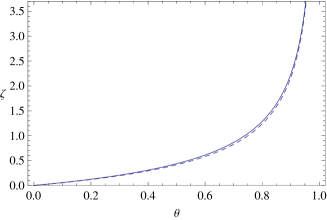
Figure 2: Solid line: efficiency $\zeta$ of the optimized refrigerator versus the temperature ratio $\theta=T_{c}/T_{h}$ for $n=3$; see (11). In the scale of this figure $\zeta(n=2)$ and $\zeta(n=3)$ are almost indistinguishable. Dashed line: the lower bound $\frac{1}{\sqrt{1-\theta}}-1$.

Thus, neither $Q_{c}$ nor $\zeta$ are good target quantities for determining an optimal regime of refrigeration. But $\chi\equiv Q_{c}\zeta$ is such a target quantity, as will be seen shortly. This is the most natural choice for our setup. This choice was also employed in yan_chen . Refs. unified ; feldman report on other approaches to defining the optimal refrigeration.

The numerical maximization of $\chi=\zeta Q_{c}$ over $\{\varepsilon_{k}\}_{k=2}^{n}$, $\{\mu_{k}\}_{k=2}^{n}$ and ${\cal U}$ has been carried out for $n=1,\ldots,5$ along the above lines. It produced the same structure: both ${\rm\bf H}$ and ${\rm\bf C}$ have $n-1$ times degenerate upper levels, see (9), and the optimal ${\cal U}$ again corresponds to SWAP operation. We thus get for $\chi=\zeta Q_{c}$ [see (10, 11)]

$$\chi(\bar{u},\bar{v})=\frac{T_{c}\theta(n-1)(\bar{v}-\bar{u})\ln^{2}\frac{1}{\bar{v}}}{[\ln\frac{1}{\bar{u}}-\theta\ln\frac{1}{\bar{v}}][1+(n-1)\bar{u}][1+(n-1)\bar{v}]},$$ (12)

where $\bar{u}$ and $\bar{v}$ are found from maximizing $\chi(u,v)$ via $\partial_{u}\chi=\partial_{v}\chi=0$. Though we have numerically checked these results for $n\leq 5$ only, we again trust that they hold for an arbitrary $n$ (one can, of course, always consider the above structure of energy spacings and ${\cal U}$ as a useful ansatz). Note that $\bar{u}$ and $\bar{v}$ depend on $\theta=T_{c}/T_{h}$. The efficiency $\zeta$ and the transferred heat $Q_{c}$ are given by (11) and (10) with $u\to\bar{u}$ and $v\to\bar{v}$; see Fig. 2.

Since the state of ${\rm\bf H}+{\rm\bf C}$ after the action of $V(t)$ is $\sigma\otimes\rho$, and because in the optimal regime the upper level for both ${\rm\bf H}$ and ${\rm\bf C}$ is $n-1$ times degenerate, one can introduce non-equilibrium temperatures $T_{h}^{\prime}$ and $T_{c}^{\prime}$ for respectively ${\rm\bf H}$ and ${\rm\bf C}$ via $\rho\propto e^{-\beta_{h}^{\prime}H_{\rm\bf H}}$ and $\sigma\propto e^{-\beta_{c}^{\prime}H_{\rm\bf C}}$. Thus, $\beta_{h}^{\prime}=\frac{1}{\bar{\varepsilon}}\ln\frac{1}{\bar{v}}$ and $\beta_{c}^{\prime}=\frac{1}{\bar{\mu}}\ln\frac{1}{\bar{u}}$, where $\bar{v}=e^{-\beta_{c}\bar{\mu}}$ and $\bar{u}=e^{-\beta_{h}\bar{\varepsilon}}$; see (9). This implies $T_{c}T_{h}=T^{\prime}_{c}T^{\prime}_{h}$. As expected, the refrigeration condition $\bar{v}>\bar{u}$, see (10, 12), is equivalent to $T_{c}^{\prime}<T_{c}<T_{h}<T_{h}^{\prime}$, i.e., the cold system gets colder, while the hot system gets hotter. Note that the existence of temperatures $T^{\prime}_{c}$ and $T^{\prime}_{h}$ was not imposed, they emerged out of optimization.

We eventually focus on two important limits: quasi-equilibrium regime $\theta\to 1$, and the macroscopic regime $\ln n\gg 1$.

In the quasi-equilibrium regime

$$\chi(a)|_{\theta=1}=T_{c}\,\theta(n-1)\,{[1+(n-1)a]^{-2}}\,\ln^{2}{a},$$ (13)

maximizes for $\bar{u}=\bar{v}=a$, where $a$ is found from $\partial_{a}\chi(a)|_{\theta=1}=0$:

$$[{(n-1)a-1}]\,\ln a=2[{(n-1)a+1}]$$ (14)

We now work out the optimal $\bar{u}$ and $\bar{v}$ for $\theta\to 1$. It can be seen from (12) that the proper expansion parameter for $\theta\to 1$ is $x\equiv\sqrt{1-\theta}$. We represent $\bar{u}$ and $\bar{v}$ as

$$\bar{u}=a+{{\sum}}_{k=1}a_{k}x^{k},~{}~{}~{}\bar{v}=a+{{\sum}}_{k=1}(a_{k}+b_{k-1})x^{k}.$$

Substituting these expressions into $\partial_{u}\chi=0$ and $\partial_{v}\chi=0$ and expanding these over $x$ we note that $a_{k}$ and $b_{k}$ are determined by equating the ${\cal O}(x^{k})$ terms:

$$b_{0}=a\ln\frac{1}{a},\quad a_{1}=-\frac{a}{2}\ln\frac{1}{a},\quad b_{1}=-\frac{a}{48}\ln\frac{1}{a}[24+\ln^{2}a].$$

This implies for the efficiency at $\theta\to 1$ ($x=\sqrt{1-\theta}$)

$$\zeta=\frac{1}{x}-1+\frac{\ln^{2}a}{48}-\frac{[48+\ln^{2}a]\ln^{2}a}{1536}\,x+{\cal O}(x^{2}).$$ (15)

Note that the expansion (15) does not apply for $n\to\infty$, since $\ln a$ diverges in this limit; see (14).

Eq. (15) suggests that $\frac{1}{\sqrt{1-\theta}}-1$ is a lower bound for the efficiency at the maximal $\chi$. This is numerically checked to be the case for all $0<\theta<1$ and all $n$; see also Fig. 2. Recalling (11) and our discussion after (12), we can interpret the lower bound for the efficiency as a lower bound on the intermediate temperature $T^{\prime}_{c}$ of ${\rm\bf C}$: $\frac{1+\sqrt{1-\theta}}{\theta}<\frac{T^{\prime}_{c}}{T_{c}}<1$, i.e., $T_{c}^{\prime}$ cannot be too low.

The macroscopic regime of a $n$-level quantum system means $\ln(n-1)\gg 1$, since for $N\gg 1$ weakly coupled particles the number of energy levels scales as $e^{N}$. Now $\bar{u}$ and $\bar{v}$ in (12) are sought via the following asymptotic expansions ($m\equiv n-1$)

$$\bar{u}={{\sum}}_{k=1}{\rho_{k}}{[m\ln m]^{-k}},~{}~{}\bar{v}={{\sum}}_{k=1}\omega_{k}m^{-k}\ln^{k}m,$$ (16)

where $\rho_{k}$ and $\omega_{k}$ are found from substituting (16) into $\partial_{u}\chi=0$ and $\partial_{v}\chi=0$ and using $\ln(n-1)\gg 1$. In the first order we get $\rho_{1}=\frac{1}{1-\theta}$, $\omega_{1}=\frac{1-\theta}{2-\theta}$, which leads to

$$\zeta=\frac{\theta}{1-\theta}-\frac{2\theta}{(1-\theta)^{2}}\frac{\ln[\ln m]}{\ln m}+{\cal O}\left[\frac{1}{\ln^{2}m}\right],$$ (17)

$$\frac{Q_{c}}{T_{c}}=\ln m-\frac{3-\theta}{1-\theta}-\ln\left[\frac{1-\theta}{2-\theta}\,\ln m\right]+{\cal O}\left[\frac{1}{\ln m}\right],$$

It is seen that in the macroscopic limit the efficiency converges to the Carnot value, while the transferred heat $Q_{c}$ is (in the leading order) a product of the colder temperature $T_{c}$ and the ”number of particles” $\ln(n-1)$. Note that the obtained attainability of the Carnot bound is related to a finite power and a finite $Q_{c}$. We see that the macroscopic limit does not commute with the equilibrium limit, since the corrections in (17) diverge for $\theta\to 1$.

Classical limit. A maximization of $\chi=Q_{c}\zeta$ can be carried out imposing equidistant spectra $\varepsilon_{n}=n\varepsilon$ and $\mu_{n}=n\mu$ for ${\rm\bf H}$ and ${\rm\bf C}$. We find that the optimal ${\cal U}$ again corresponds to SWAP operation. Thus, for $\chi=\chi(\bar{u},\bar{v})$ we obtain

$$\chi=\frac{T_{c}\theta\ln^{2}\frac{1}{\bar{v}}}{\ln\frac{1}{\bar{u}}-\theta\ln\frac{1}{\bar{v}}}\left[\frac{\bar{v}-\bar{u}}{(1-\bar{v})(1-\bar{u})}-\frac{n(\bar{v}^{n}-\bar{u}^{n})}{(1-\bar{v}^{n})(1-\bar{u}^{n})}\right],$$

where $\bar{v}=e^{-\beta_{c}\bar{\varepsilon}}$ and $\bar{u}=e^{-\beta_{h}\bar{\mu}}$ are found from maximizing $\chi$. The efficiency $\zeta$ is still given by (11). In the limit $n\gg 1$ we get from (Optimal thermal refrigerator.): $\bar{u}\to 1$, $\bar{v}\to 1$ and $\frac{n(\bar{v}^{n}-\bar{u}^{n})}{(1-\bar{v}^{n})(1-\bar{u}^{n})}\to 0$. Both $\chi$ and $\zeta$ depend on one parameter $\phi\equiv\frac{1-\bar{u}}{1-\bar{v}}$, whose optimal value is $\phi=1+\sqrt{1-\theta}$. We get in this limit: $\chi=\frac{T_{c}\theta}{(1+\sqrt{1-\theta})^{2}}$ and $\zeta=\frac{1}{\sqrt{1-\theta}}-1$. Thus for a large number of equidistant energy levels (macro-limit) the optimal regime now implies homogeneity ($\bar{\varepsilon}\to 0$, $\bar{\mu}\to 0$), which is an indication of the classical limit: under this conditional optimalization the efficiency $\zeta$ is exactly equal to the [unconditional] lower limit $\zeta_{\rm CA}=\frac{1}{\sqrt{1-\theta}}-1$.

In conclusion, we have studied a model of a refrigerator aiming to understand its optimal performance at a finite cooling power; see Fig. 1. The structure of the model is such that it can be optimized over almost all its parameters; additional constraints can and have been considered, though. We have confirmed an incompatibility between optimizing the heat $Q_{c}$ transferred from the cold bath $T_{c}$ and efficiency $\zeta$: Maximizing one nullifies the other. A similar effect for a different model of quantum refrigerator has been reported in segal .

To get a balance between $Q_{c}$ and $\zeta$ we have thus chosen to optimize their product $\zeta Q_{c}$. This leads to a lower bound $\zeta_{\rm CA}=\frac{1}{\sqrt{1-\theta}}-1$ ($\theta\equiv\frac{T_{c}}{T_{h}}$) for the efficiency in addition to the upper Carnot bound $\zeta_{\rm C}=\frac{1}{1-\theta}-1$. The Carnot upper bound is reached (at a finite power and finite $Q_{c}$!) in the macroscopic (many-level) limit of the model. To our knowledge such an effect has never been seen so far for refrigerator models. For the optimal refrigerator the transferred heat $Q_{c}$ behaves as $Q_{c}\propto T_{c}$ for $T_{c}\to 0$; see (10, 12, 17). This is in agreement with the optimal low-temperature behaviour of $Q_{c}$ from the viewpoint of the third law rezek . The lower bound $\zeta_{\rm CA}$ is reached in the equilibrium limit $T_{c}\to T_{h}$. Constraining both systems to have homogeneous (classical) spectra, $\zeta_{\rm CA}$ is reached as an upper bound. This is just like within finite-time thermodynamics (FTT), when maximizing the product of the cooling-power and efficiency yan_chen , or the ratio of the efficiency and the cycle time velasco . In this sense $\zeta_{\rm CA}$ seems to be universal. It may play the same role as the Curzon-Ahlborn efficiency for heat engines $\eta_{\rm CA}$, which, again, is an upper bound within FTT ca ; broek , but appears as a lower bound for the engine models studied in armen ; tu ; izumida_okuda . Other opinions on the Curzon-Ahlborn efficiency for refrigerators are given in jimenez ; unified .

This work has been supported by Volkswagenstiftung.

References

• (1) H.B. Callen, Thermodynamics (John Wiley, NY, 1985).
• (2) J. Gemmer, M. Michel and G. Mahler, Quantum Thermodynamics (Springer, 2004).
• (3) V. Balzani, A. Credi and M. Venturi, Molecular Devices and Machines (Wiley-VCH, Weinheim, 2003).
• (4) R.S. Berry et al. Thermodynamic Optimization of Finite–Time Processes (John Wiley & Sons, Chichester, 2000).
• (5) F. Curzon and B. Ahlborn, Am. J. Phys. 43, 22 (1975). H. Leff, Am. J. Phys. 55, 602 (1987).
• (6) C. Van den Broek, Phys. Rev. Lett. 95, 190602 (2005).
• (7) R. Kosloff, J. Chem. Phys. 80, 1625 (1984).
• (8) A.E. Allahverdyan et al., Phys. Rev. E 77, 041118 (2008).
• (9) Z.C. Tu, J. Phys. A 41, 312003 (2008).
• (10) Y. Izumida and K. Okuda, EPL 83, 60003 (2008).
• (11) T. Schmiedl and U. Seifert, EPL 81, 20003 (2008).
• (12) M. Esposito, et al., Phys. Rev. Lett. 102, 130602 (2009).
• (13) A.E. Allahverdyan et al., J. Mod. Opt. 51, 2703 (2004).
• (14) M.J. Henrich et al., Europhys. Lett., 76, 1057 (2006).
• (15) Z. Yan and J. Chen, J. Phys. D 23, 136 (1990).
• (16) S. Velasco et al., Phys. Rev. Lett. 78, 3241 (1997).
• (17) B. Jimenez de Cisneros et al., Phys. Rev. E 73, 057103 (2006).
• (18) A. Calvo Hernandez et al., Phys. Rev. E 63, 037102 (2001).
• (19) T. Feldman and R. Kosloff, Phys. Rev. E, 61, 4774 (2000).
• (20) D. Segal, Phys. Rev. Lett. 101, 260601 (2008).
• (21) Y. Rezek et al., EPL, 85, 30008 (2009).
• (22) A.W. Marshall and I. Olkin, Inequalities (Academic Press, New York, 1979).