Statistical Aspects of Baseline Calibration in Earth-Bound Optical Stellar Interferometry

Abstract

Baseline calibration of a stellar interferometer is a prerequisite to data reduction of astrometric operations. This technique of astrometry is triangulation of star positions. Since angles are deduced from the baseline and delay side of these triangles, length and pointing direction (in the celestial sphere) of the baseline vector at the time of observation are key input data. We assume that calibration follows from reverse astrometry; a set of calibrator stars with well-known positions is observed and inaccuracies in these positions are leveled by observing many of them for a common best fit.

The errors in baseline length and orientation angles drop proportional to the inverse square roots of the number of independent data taken, proportional to the errors in the individual snapshots of the delay, and proportional to the errors in the apparent positions of the calibrators. Scheduling becomes important if the baseline components are reconstructed from the sinusoidal delay of a single calibrator as a function of time.

I Overview

Astrometry as realized by a contemporary optical stellar interferometer is founded on the sensitivity to wave front tilts of stellar light, which leads to a dephasing proportional to the tilt and proportional to the distance between the two telescope’s apertures. This is measured by the amount of delay—in units of time or optical path length difference—added by the observatory’s optical infrastructure to the beam hitting the telescope closer to the star to adjust the phase difference of the light beams for close-to-coherent superposition at the detector.

We only address geometry in this manuscript. The wealth of non-statistical effects of tidal Earth-crust motion, Earth axis drifts McCarthy and Petit (2003); Capitaine et al. (2003, 2005); Lambert (2003, 2006); Kaplan (2006), aberration and general-relativistic wavefront tilts which leave residual noise once the known quantities are accounted for is left aside.

Mathematics of small differences demonstrates in Section II how measurement of the difference in the delay defined by an angular separation of two “science” objects in the celestial sphere requests some knowledge of the baseline vector—which we vaguely define as the separation between the two input pupils of the two telescopes involved. Baseline calibration is the auxiliary observation of well-known (in the astrometric sense) calibrator stars to deduce this baseline geometry.

On can think of two pure forms. First there is a Fourier mode which matches the sinusoidal delay as a function of time with the three free parameters of the baseline vector tracking an individual star (Section III). This minimizes the time overhead of slewing/pointing/acquisition/fringe-loop-lock cycles. A characteristic sensitivity of the baseline parameters means that is is favorable to reserve time slots six hours apart Saunders et al. (2006).

This compares to the second form—which one may call field mode—in which delays of a larger set of calibrator stars covering a wide range of altitudes and azimuths are gathered (Section IV).

The topic of this script is focused on the narrow question: given statistical errors of the delay measurement in Fourier mode and statistical errors in positions derived from star catalogs in the field mode, how long or how many of them, respectively, does the calibration need to balance their effect to the levels set by the astrometric mode.

II Fundamental Trigonometry

II.1 Daily OPD

We start with a summary of the fundamental geometry of observing a star with perfectly stable telescopes orbiting a fixed Earth axis without atmospheric or similar distortions Mathar (2008).

The terrestrial coordinate system defines geographic longitude $\lambda$, latitude $\phi$ and altitude $H$ of two telescopes. By conversion into a Cartesian frame and construction of the mid-point between any pair of these, we define the geographic longitude $\lambda$ and geographic latitude $\phi$ of the baseline, which serves to define the topocentric Alt-Az system for the baseline—which implies that $a_{b}=0$ since we define an individual system for each pair. In this topocentric coordinate system, the baseline vector has length $b$ and splits into Cartesian coordinates

$${\mathbf{b}}=b\left(\begin{array}[]{cc}-\cos A_{b}\cos a_{b}\\ \sin A_{b}\cos a_{b}\\ \sin a_{b}\end{array}\right)$$ (1)

as a function of azimuth $A_{b}$ (South over West) and inclination $a_{b}$. A rotation matrix $U$

$$U\equiv\left(\begin{array}[]{ccc}-\sin\phi\cos\lambda&-\sin\phi\sin\lambda&\cos\phi\\ \sin\lambda&-\cos\lambda&0\\ \cos\phi\cos\lambda&\cos\phi\sin\lambda&\sin\phi\end{array}\right)$$ (2)

transforms these coordinates to Cartesian coordinates in a geocentric frame for suitably defined celestial declination $\delta_{b}$ and hour angle $h_{b}$ Mathar (2008),

$${\mathbf{b}}=U\cdot b\left(\begin{array}[]{cc}\cos\delta_{b}\cos(\lambda-h_{b})\\ \cos\delta_{b}\sin(\lambda-h_{b})\\ \sin\delta_{b}\end{array}\right).$$ (3)

Table 1 illustrates this transformation for a Chilean site. (The constant height $H$ above the ellipsoid implies that neither telescopes nor baselines are co-planar.)

The direction to the star of right ascension $\alpha$ and declination $\delta$ at current azimuth $A$ and zenith angle $z$ is

$${\bf s}=\left(\begin{array}[]{c}-\cos A\sin z\\ \sin A\sin z\\ \cos z\\ \end{array}\right)=U\cdot\left(\begin{array}[]{c}\cos\delta\cos(\lambda-h)\\ \cos\delta\sin(\lambda-h)\\ \sin\delta\end{array}\right).$$ (4)

Table 1: A model of telescope coordinates and the associated equatorial variables of the Very Large Telescope Interferometer aligned with WGS84 conventions.

telescope	$\lambda$ (rad)	$\phi$ (rad)	$H$ (m)
U1	$-1.228800386$	$-0.429833092$	$2635.43$
U2	$-1.228796107$	$-0.429825122$	$2635.43$
U3	$-1.228790929$	$-0.429819523$	$2635.43$
U4	$-1.228780856$	$-0.429823005$	$2635.43$

baseline	$b$	$\lambda$	$\phi$	$A_{b}$	$\delta_{b}$	$h_{b}$
	(m)	(deg)	(deg)	(deg)	(deg)	(deg)
U12	$56.4$	$-70.4050$	$-24.8342$	$-153.9$	$46.8$	$-49.7$
U13	$102.1$	$-70.4048$	$-24.6272$	$-147.5$	$43.9$	$-56.8$
U14	$130.2$	$-70.4045$	$-24.6273$	$-119.5$	$25.6$	$-76.8$
U23	$46.5$	$-70.4047$	$-24.6270$	$-139.8$	$39.8$	$-63.8$
U24	$89.5$	$-70.4044$	$-24.6271$	$-98.6$	$7.8$	$-86.4$
U34	$62.5$	$-70.4042$	$-24.6269$	$-69.3$	$-18.4$	$-99.0$

The equation-of-motion of the optical path difference (OPD) $D$ is Mathar (2008)

$$D={\bf s}\cdot{\bf b} = b\left[\cos z\sin a_{b}+\sin z\cos a_{b}\cos(A-A_{b})\right]$$ (5)

$$= b\left[\sin\delta\sin\delta_{b}+\cos\delta\cos\delta_{b}\cos(h-h_{b})\right].$$

This is the common spherical coordinates formula for the angular distance between two points, one fixed at $(\alpha,\delta)$, the other at fixed $\delta_{b}$ cycling the polar axis in one sidereal day $T_{d}$, at an angular velocity of

$$\omega_{d}=2\pi/T_{d}\approx 73\,\mu\mathrm{rad/s}.$$ (6)

The characteristic parameters of $D(h)$ are sketched in Figure 1: a time-independent offset $b\sin\delta\sin\delta_{b}$, an amplitude $b\cos\delta\cos\delta_{b}$, and a phase $h_{b}$.

Figure 1: Equation (5) generates a periodic delay in time.

The baseline length $b$ and the angles $\delta_{b}$ and $h_{b}$ are encoded in phase and amplitude of $D$ plotted over time $t$.

The time-dependent projected baseline angle $p_{b}$ is the position angle of high sensitivity of $D$ to changes in the sky coordinates, that is the direction of high interferometric resolution Mathar (2008),

$$\tan p_{b}=\frac{\cos\delta_{b}\sin(h-h_{b})}{\cos\delta\sin\delta_{b}-\sin\delta\cos\delta_{b}\cos(h-h_{b})}.$$ (7)

II.2 Differential OPD

We are concerned with differential astrometry of observing two objects at a single point in time rather than switching between the two stars van Belle et al. (2008); Armstrong et al. (1998). We note (5) for two stars with coordinates $\delta_{i}$ and $\alpha_{i}=LST-h_{i}$, mean positions $\bar{\delta}$ and $\bar{\alpha}$,

$$\Delta\alpha \equiv \alpha_{2}-\alpha_{1};\quad\bar{\alpha}\equiv(\alpha_{2}+\alpha_{1})/2;$$ (8)

$$\Delta\delta \equiv \delta_{2}-\delta_{1};\quad\bar{\delta}\equiv(\delta_{2}+\delta_{1})/2.$$ (9)

$$\bar{h} \equiv (h_{2}+h_{1})/2=LST-\bar{\alpha}.$$ (10)

The time-independent cosine of the angular separation $\tau$ is

$$\cos\tau = \cos\delta_{1}\cos\delta_{2}\cos(\alpha_{1}-\alpha_{2})+\sin\delta_{1}\sin\delta_{2}$$ (12)

$$\approx 1-\frac{1}{2}(\Delta\delta)^{2}-\frac{1}{2}\cos^{2}\bar{\delta}(\Delta\alpha)^{2}+\frac{1}{24}(\Delta\delta)^{4}$$

$$+\frac{1}{8}(\Delta\delta)^{2}(\Delta\alpha)^{2}+\frac{1}{24}\cos^{2}\bar{\delta}(\Delta\alpha)^{4}+\cdots$$

in these coordinates, neglecting sixth and higher order mixed differentials. The differential OPD becomes a sinusoidal function of time, too,

$$\Delta D=D_{2}-D_{1}=({\bf s}_{2}-{\bf s}_{1})\cdot{\bf b}\equiv o+p\cos(\bar{h}-h_{b}+h_{0}),$$ (13)

which defines a coordinate offset $o$, a daily amplitude $p$, and a time shift $h_{0}$ (Fig. 2).

Figure 2: Equation (13) defines a differential delay with the same period length as the wide-angle delays $D_{1}$ and $D_{2}$.

For small $\Delta\alpha$ and small $\Delta\delta$, up to fourth order in $\Delta\delta$,

$$o\approx b\Delta\delta\cos\bar{\delta}\sin\delta_{b}-\frac{1}{24}b(\Delta\delta)^{3}\cos\bar{\delta}\sin\delta_{b}.$$ (14)

Up to fifth mixed order in the differentials we have the squared amplitude of the differential delay,

$$p^{2} \approx b^{2}\cos^{2}\delta_{b}\big{[}\sin^{2}\bar{\delta}(\Delta\delta)^{2}+\cos^{2}\bar{\delta}(\Delta\alpha)^{2}-\frac{1}{12}\sin^{2}\bar{\delta}(\Delta\delta)^{4}$$ (15)

$$-\frac{1}{12}\cos^{2}\bar{\delta}(\Delta\alpha)^{4}-\frac{1}{4}(\Delta\delta)^{2}(\Delta\alpha)^{2}\big{]},$$

and the shift in hour angle

$$\tan h_{0}\approx\cot\bar{\delta}\frac{\Delta\alpha}{\Delta\delta}\big{[}1-\frac{1}{12}(\Delta\delta)^{2}+\frac{1}{12}(\Delta\alpha)^{2}$$

$$-\frac{1}{720}(\Delta\delta)^{4}-\frac{1}{144}(\Delta\delta)^{2}(\Delta\alpha)^{2}+\frac{1}{120}(\Delta\alpha)^{4}\big{]}.$$ (16)

The right hand side contains a factor $\cos\bar{\delta}\Delta\alpha/\Delta\delta$, the tangent of the position angle of the binary to lowest order in the differentials.

II.3 Correlation of Variables

The astronomer’s interest of astrometric operations is in the measurement in the two parameters that characterize the relative position of the binary’s components on the sky, which could either be represented as $\Delta\alpha$ and $\Delta\delta$, or alternatively as distance $\tau$ and position angle.

From a fit to a sine model like (13), a measurement can extract three parameters, which represent the six free Cartesian components of head and tail of the baseline vector minus the degrees of freedom of the three components of the baseline center (which represent a free rigid translation of the baseline and do not contribute to the interferometric signal).

For the purpose of this script, the time base is not considered an independent source of error. (On a real-time bus an individual query for a time stamp has a resolution of roughly 10 $\mu$s, i.e., $150$ $\mu$as after multiplication by $\omega_{d}$. Micro-controller boards usually govern the readout process, so the jitter is much smaller.)

These three parameters could either be stored as Cartesian coordinates of the baseline vector, or in the coordinates $b$, $\delta_{b}$ and $h_{b}$ which are more meaningful in the context of the analysis of $D(t)$ in general.

Independent of this question of format, there is some redundancy between the three fitting parameters $o$, $p$ and $h_{0}$ contained in $D(t)$ and the two positional parameters of the binary, supposed an independent baseline calibration provides the auxiliary $b$, $\delta_{b}$ and $h_{b}$. The task of the baseline calibration is to support inversion of equations (14)–(16). From this point of view, we need the product $b\sin\delta_{b}$ to reduce (14), the product $b\cos\delta_{b}$ to reduce (15), and $h_{b}$ to reduce (16).

If one of the three equations is not activated for some reason, one of these three projections of the baseline vector (onto the polar axis and on the equatorial plane) does not need to be calibrated either, because —in principle—two equations for two unknowns remain. The U24 baseline in Table 1 provides an example of this aspect, where $b\sin\delta_{b}\approx 12$ m. The factor $\cos\bar{\delta}$ might reduce the product $b\cos\bar{\delta}\sin\delta_{b}$ on the right hand side of (14) to only $6$ m, which couples an accuracy of 100 $\mu$as$=5\times 10^{-10}$ rad in $\Delta\delta$ to an accuracy in $o$ of 3 nm. If the astrometric run cannot meet this requirement, equation (14) drops out of the data reduction process, and in turn, the value $b\sin\delta_{b}$ is not requested from the baseline calibration. If the value of $b\cos\delta_{b}$ is very small, equation (15) may become disposable with the same rationale.

From a similar mathematical but entirely different engineering point of view, the measurement of $D$ will likely be assisted by a metrology system which is difficult to calibrate over longer periods of time (which includes drifts of air densities if operating in air and atmospheric lensing effects) and is difficult to run without interruption. The time derivative, i.e, the delay velocities

$$\Delta\dot{D}(t)=-p\omega_{d}\sin(\bar{h}-h_{b}+h_{0}),$$ (17)

$$\dot{D}(t)=-b\omega_{d}\cos\delta\cos\delta_{b}\sin(h-h_{b})$$ (18)

will be available more easily, but this eliminates the offset, including the differential offset $o$ and (14), as an independent piece of information.

II.4 Requested Baseline Accuracy

The “cushion” and “barrel” distortions of the geometry by the cubic terms of (14) and biquadradic terms of (15) and (16) are usually negligible: If the angular distance is limited by some finite field-of-view to $\tau\lesssim 2^{\prime}$, the squares are limited to $\tau^{2}\lesssim 3\times 10^{-7}$ rad². If the other terms in the sum are of the order of unity, these higher order contributions change $\Delta\delta$ or $\Delta\alpha$ by less than $2^{\prime}\times 3\times 10^{-7}\approx 40$ $\mu$as.

So requirements on the baseline calibration can be derived from the first orders $o\sim b\Delta\delta\cos\bar{\delta}\sin\delta_{b}$ and $p\sim b\cos\delta_{b}\sin\bar{\delta}\Delta\delta$ $\sim b\cos\delta_{b}\cos\bar{\delta}\Delta\alpha$. In a broad sense the relative error in $\Delta\delta$ and $\Delta\alpha$ is of the order of the relative error in $o$ plus the relative error in $b\sin\delta_{b}$, or $p$ plus the relative error in $b\cos\delta_{b}$, respectively. As a guideline: an accuracy of 100 $\mu$as in a field of $\tau<2^{\prime}$, or 10 $\mu$as in a field of $\tau<10^{\prime\prime}$, is equivalent to a relative accuracy of $1\times 10^{-6}$, which splits evenly into requirements of $5\times 10^{-7}$ in $o$ ($p$) and $b$, which is a requirement of 50 $\mu$m for a baseline of $b=100$ m of length.

Equivalent considerations are available for (18): The relative error in the value of $b$ matches the relative error in the value of $\dot{D}$. For an error 50 $\mu$m in a 100 m baseline we need a relative accuracy of $\dot{D}$ of $5\times 10^{-7}$. Since the speed is of the order 1 cm/s for a 100 m baseline, we want to have $\dot{D}$ in absolute precision to $5\times 10^{-9}$ m/s = 5 nm/s. Near the turning points $h\approx h_{b}$, the requirements for absolute precision become tighter, enforced by the sine factor in (18).

The signal $\dot{D}(t)$ may also be small because either $\delta$ or $\delta_{b}$ are near 90^∘, which puts higher stress on the measurement of the absolute value of this velocity. The effect through $\cos\delta$ means that a star on a closed apparent orbit around the corresponding celestial pole of the observatory’s hemisphere induces a small variation of delay because its apparent position does not change much anyway. The effect through $\cos\delta_{b}$ punishes North-South baselines of observatories near the equator because $\delta_{b}$ measures the angle between the baseline and the equatorial plane.

To keep the number of parameters basically down to three, this manuscript does not introduce models of telescope axes runouts as a function of azimuth and altitude. They do have an impact on the calibration: a runout of 50 $\mu$m by one of the telescopes, i.e., not matched by the other, is equivalent to that characteristic baseline tilt of 100 mas over $b=100$ m mentioned above.

III Tracking a Single Star

III.1 3-parametric fit

The simplest scheme to derive baseline coordinates from reverse wide-angle astrometry is to monitor the trace for a single star, as in Fig. 1, over a significant portion of one of the periods.

One reason for such a strategy can be that there are few calibrator stars with small errors in their $(\alpha,\delta)$ coordinates and mixture with data from more stars—strategy of Section IV—could deteriorate the statistics. Another reason is enhanced efficiency if the calibrator star is one of the components of the binary system; baseline calibration and astrometric observation may then run concurrently if delay and differential delay data are recorded simultaneously.

A Fourier analysis can extract amplitude, offset and phase by a least-squares fit

$$\sum_{j=1}^{N}[b\sin\delta\sin\delta_{b}+b\cos\delta\cos\delta_{b}\cos(h_{j}-h_{b})-D_{j}]^{2}\rightarrow\mathrm{min}$$ (19)

by $N$ measurements. The individual delay measurements $D_{j}$ are characterized by an error variance $\sigma^{2}(D)$. One might include some statistical weights of the squares in (19) by some inverse function of the projected baseline—which represents the angular resolution of the interferometer—but this adds more parameters to the present analysis and obscures the principles laid out below.

The output (and free parameters) of the fitting process are $b\sin\delta_{b}$ (polar component of the baseline), $b\cos\delta_{b}$ (equatorial component of the baseline) and $h_{b}$ (interferometric hour angle). The error propagation of such a Fourier analysis has been discussed in the literature (Smart, 1958, §7.04)Rice (1954); Goldberg and Bokor (2001). There is no need to split the components into length $b$ and angle $\delta_{b}$ for two reasons:

1. These are correlated variables. There is no profit from dividing the information (plus tracking the covariances), to re-unite them afterwards for application in (14) and (15).

2. If the the observable is the delay velocity $\dot{D}$ and the differential delay velocity $\Delta\dot{D}$ as discussed above, the components remain properly separated. One can basically ignore the error analysis of the offsets (polar components).

III.2 Scheduling

The limits of observing during the night and observing stars at some minimum altitude above the horizon lead to a characteristic error propagation depending on which portion of the delay is covered by the observation. As sketched in Fig. 3, $N$ observations of snapshots $D_{j}$ would start at some time $\varphi_{0}$ after the daily maximum. The quality of the fit to the amplitude or offset depends on whether $\varphi$ is near zero or $\pi$ on one hand, or $\pi/2$ away from a maximum or minimum on the other hand.

Figure 3: The baseline calibration in Fourier mode samples the delay of Fig. 1 at points $j=1,2,\ldots N$ in time, starting at $\varphi_{0}$.

We summarize simple Monte Carlo calculations of these dependencies in Figures 4–6 for a baseline of $b=100$ m.

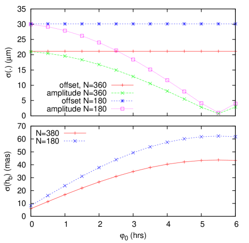
Figure 4: Errors to the delay offset, delay amplitude and delay hour angle for $N=360$ measurements in intervals of 10 seconds or $N=180$ measurements in intervals of 20 seconds (an observation taking one hour). $\sigma(D)=1$ $\mu$m for each measurement.

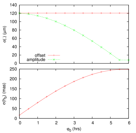
Figure 5: Errors to the three parameters of Fig. 4 for $N=180$ measurements in intervals of 10 seconds, covering only the next half an hour after $\varphi_{0}$.

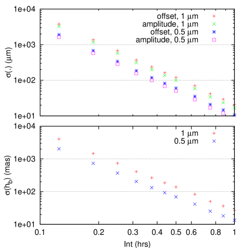
Figure 6: Errors to the three parameters for measurements at intervals of 10 seconds, total integration time from 0.1 to 1 hour, $\sigma(D)=1$ $\mu$m or 0.5 $\mu$m, $\varphi_{0}=2$ hrs.

The common feature of Fig. 4 and 5 is:

• The quality of the measure of the offset (mean) does not depend on when the observation is started.

• The amplitude of the curve is obtained with highest quality if the observation covers the part of maximum delay velocity. To achieve highest precision in the hour angle, however, the observation ought to cover the part of zero velocity near an extremum, six or eighteen hours earlier or later.

Fig. 4 shows the generic dependency of errors $\sim N^{-1/2}$ if duration and time slot of the observation stay the same. The transition from Fig. 4 to Fig. 5 demonstrates that cutting the observation time by half, keeping the detector integration time the same, increases the errors by an approximate factor of six. Fig. 6 emphasizes this dependence of the errors $\sim N^{-5/2}$ (at constant detector integration time), but confirms the expected proportionality to the error $\sigma(D)$ of the individual readout.

In this model, the error $\sigma(D)$ is an effective superposition of an error induced by the error in the interferometric phase plus an error from the jitter in the time base. At velocities $\dot{D}<1$ cm/s, an error of $\sigma(h)=20$ $\mu$s in the time base is equivalent to an error $\sigma(D)=\dot{D}\sigma(h)<200$ nm, for example. Techniques to reduce this error by implementing detector-readout schedules in low-level micro-controller programs are not in the scope of this paper.

IV Calibrator Star Catalog Imprecision

IV.1 Baseline Length Calibration

The estimated error $\sigma(b)$ in the baseline length for $b=100$ m obtained by a 1-parametric least squares fit after visiting $N$ stars on the sky that are rather homogeneously distributed in the range $z<60^{\circ}$ is shown in Figure 7. The $N$ positions are randomly selected over the sky in the zenith range $z<60^{\circ}$, taking subsets of the Hardin-Sloan-Smith points Hardin et al. (1997), and have been displaced by angles with five different Gaussian widths between $0.025^{\prime\prime}$ and $0.4^{\prime\prime}$ to generate a measured delay, to which in addition errors of $\sigma(D)=100$ nm or $\sigma(D)=2$ $\mu$m are added. Double logarithmic axes scales are chosen to verify that the reduction in $\sigma(b)$ is approximately proportional to $N^{-1/2}$.

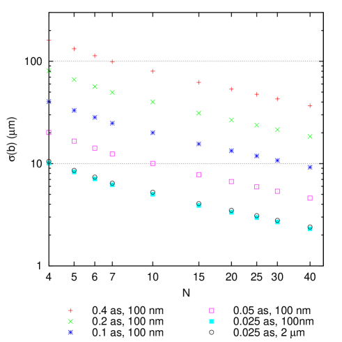
Figure 7: The error $\sigma(b)$ to a baseline length $b=100$ m from a least-squares fit to $N$ measured delays $D$ for $N$ stars.

Figure 8 uses a more constrained region of the sky with $z<40^{\circ}$ and achieves inferior accuracy for equivalent numbers of stars. (The side effect that the projected baseline is larger on the average than in Fig. 7 which implies better resolutions is not taken into account.)

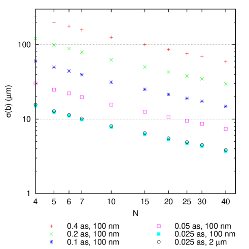
Figure 8: The errors of Figure 7 if baseline calibrator stars are only selected in the zenith range $z<40^{\circ}$.

The apparent positions of stars are effected for example by the chromatic dispersion in air, the product of the dielectric susceptibility of air Mathar (2007) at the telescope—measured in radians—and the tangent of the zenith angle. Examples for two infrared windows for Paranal conditions are plotted in Fig. 9 and 10 for three different water vapor densities.

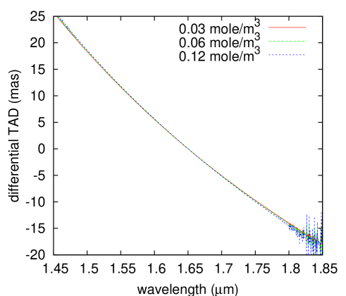
Figure 9: The chromatic differential transverse atmospheric dispersion (TAD) in the H band for $\tan z=1$ at an ambient pressure of 744 hPa, relative to a wavelength of 1.65 $\mu$m.

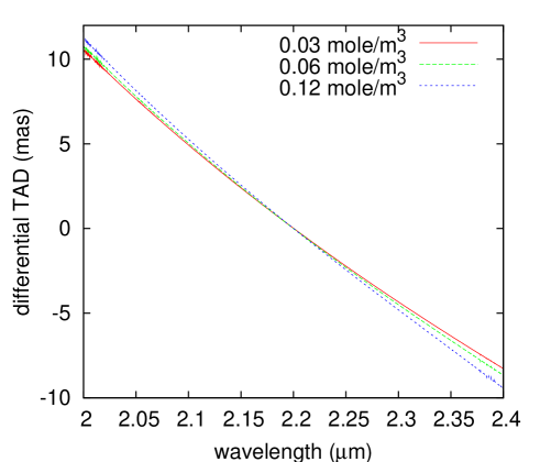
Figure 10: The differential transverse atmospheric dispersion in the K band for $\tan z=1$ at an ambient pressure of 744 hPa, relative to a wavelength of 2.2 $\mu$m.

This implicit spread of a few tens of mas depending on the star color is of the same order as extrapolation errors for the apparent position from integrated proper motions since the Hipparcos epoch Damljanović and Pejović (2008); Kovalevsky et al. (1997).

IV.2 Baseline Vector Calibration

Fig. 11 are results of a least squares fit of the 3 degrees of freedom of the baseline vector to a series of delay measurements, minimizing $\sum_{1}^{N}[D_{j}-{\bf s}_{j}\cdot{\bf b}]^{2}$ over a set of “noisy” star positions $A_{j}$ and $z_{j}$ and building a statistics over the variables $b$, $A_{b}$ and $a_{b}$. The error to the the measured delay has been set to zero, because Figs. 7–8 reveal that they are not important if they remain $\sigma(D)\lesssim 2$ $\mu$m. The $N$ positions have been rather homogeneously distributed over the sky as in Fig. 7 in the zenith range $z<60^{\circ}$, and have been randomly displaced by angles with different Gaussian widths of $0.4^{\prime\prime}$ (pluses), $0.2^{\prime\prime}$ (crosses) or $0.1^{\prime\prime}$ (stars).

The accuracy in the baseline length $b$ is the same as obtained with the 1-parameter fits of Fig. 7. Clearly, for small $N$, the error in the angles just echoes the error introduced in the star positions.

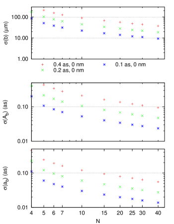
Figure 11: The error to a baseline length $b=100$ m, and to the baseline orientation angles from a 3-parametric least-squares fit measured to delays $D$ of $N$ calibrator stars.

The elevation angle $a_{b}$ (tilt of the baseline versus the horizontal) is obtained roughly twice as accurate as the azimuth $A_{b}$. The interpretation of this bias is: the even distribution of the calibrator stars along azimuths and their more clumpy, overhead distribution along zenith angles means that a measurement via the projections $D$ achieves low resolution along the horizontal for the two subsets of stars in the two opposite pointing directions of the baseline (Muterspaugh, 2005, Fig 2-8). The coupling along the vertical coordinate is stiffer on the average, and the information contained in the delays better distributed to deduce the baseline tilt (pitch) versus the horizon than the baseline rotation (roll) around the zenith.

This difference in fitting quality in the $(a_{b},A_{b})$ angles is more obscure in the $(\delta_{b},h_{b})$ system, because multiplication with the inverse (transpose) of the $U$-matrix (2) weights components depending on the geographic latitude $\phi$. Anyway, the angles in Fig. 11 are related to the effect of Earth axis pointing Kaplan (1990), which can be written down as a change of the effective ($\delta_{b},h_{b}$) coordinates. Formula (5) is in fact symmetric as one could swap the variables $\delta$ and $\delta_{b}$ or $h_{j}$ and $h_{b}$ without changing the delay. Clearly, the calibration measures a baseline orientation in an ecliptic (celestial) reference frame, not in a terrestrial reference frame. The two sides of this coin are

• Pushing errors in $a_{b}$ or $A_{b}$ below the limits set by the errors in the IERS angles www.usno.navy.mil/USNO/earth-orientation /eo-products is useless if the aim is to reduce delays to the terrestrial baseline data.

• There is a prospect of setting up a competitive optical reference frame to 40 mas—aside from the influence of all systematic effects—if $N\gtrsim 15$ stars with positions accurate to 100 mas are available. (This estimate follows almost trivially from a $N^{-1/2}$ scaling of uncorrelated errors.)

A further remark: The baseline vector calibration is in a general sense equivalent to determining the geographic longitude and latitude of either head or tail of the baseline vector: one can change the orientation of the baseline by either tilting it explicitly or keeping it always horizontal and sliding it with the tangent plane across the Earth surface. In mathematical prose: Introducing the geographic latitude $\phi$ or longitude $\lambda$ as additional fitting parameters into the minimization procedure defines an ill-conditioned problem.

V Summary

Baseline calibration reduces measurements of the scalar variable of the delay to baseline vector components along the polar and equatorial axes, and splits the equatorial component into two with the aid of clocks.

The interest is in the measure of angles, such that the requirements on lengths (delay and baseline) are not formulated in absolute but in relative units: the relative error in the star separation of the astrometric observation is the relative error in the delay measure plus the relative error in the baseline length, and similar generic statements apply separately to the components in right ascension and declination.

The statistical errors in the baseline coordinates are proportional to the errors of the individual delay (or its speed) and time stamp, and proportional to the inverse square root of the number of independent measurements, as expected. If the baseline coordinates are derived from a Fourier analysis of the delay or delay speed as a daily function of time, the statistical errors depend more decisively on schedules and on the percentage of the sidereal period that is covered.

Appendix A Tidal Motion

One contribution of the definition of the telescope coordinates in an extra-terrestrial coordinate system is given by the influence by the ocean tides that load and release the non-rigid Earth crust Sovers et al. (1998). According to the GOt00.2 model by Bos and Scherneck Bos and Scherneck (2005), the amplitude for the Paranal geographical coordinates is $<2$ cm in vertical and $<0.7$ cm in horizontal directions: Fig. 12.

Figure 12: Illustration of the vertical and lateral motion of the Earth crust at the Paranal coordinates parametrized with 11 harmonic frequencies Bos and Scherneck (2005). The fundamental mode exhibits the two daily tides, the envelope is governed by the Moon’s period.

The Earth crust motion in other regions of the planet may be up to 10 cm.

The periodic influence on astrometry can be estimated by converting the East-West motion into a change of the instantaneous geographic longitude $\lambda$, the North-South motion into a change of the geographic latitude $\phi$. A sliding by 1 cm translates into a tilt of $0.01/6.38\times 10^{6}\approx 1.5\times 10^{-9}$ rad $\approx 0.3$ mas, and is therefore not relevant for the baseline calibration if the errors in calibrator star positions are roughly one or two magnitudes larger. With a similar rationale, a change of $\bar{\delta}$ in (14) or (15) by $1.5\times 10^{-9}$ remains negligible if the request for relative errors in $o$ or $p$ is of the order $5\times 10^{-7}$ as argued in section II.4.

References

- Armstrong et al. (1998) Armstrong, J., D. Mozurkewich, L. J. Rickard, D. J. Hutter, J. A. Benson, P. F. Bowers, N. M. Elias II, C. A. Hummel, K. J. Johnston, D. F. Buscher, J. H. Clark III, L. Ha, et al., 1998, Astrophys. J. 496(1), 550.
- Bos and Scherneck (2005) Bos, M. S., and H.-G. Scherneck, 2005, The free ocean tide loading provider, URL http://www.oso.chalmers.se/~loading.
- Capitaine et al. (2005) Capitaine, N., P. T. Wallace, and J. Chapront, 2005, Astron. Astrophys. 432(1), 355.
- Capitaine et al. (2003) Capitaine, N., P. T. Wallace, and D. D. McCarthy, 2003, Astron. Astrophys. 406(3), 1135.
- Damljanović and Pejović (2008) Damljanović, G., and N. Pejović, 2008, Serb. Astr. J. 177, 109.
- Goldberg and Bokor (2001) Goldberg, K. A., and J. Bokor, 2001, Appl. Opt. 40(17), 2886.
- Hardin et al. (1997) Hardin, R. H., N. J. A. Sloane, and W. D. Smith, 1997, Tables of spherical codes, URL http://www.research.att.com/~njas/packings/.
- Kaplan (1990) Kaplan, G. H., 1990, in Inertial Coordinate Systems on the Sky, edited by J. H. Lieske and V. K. Abalakin (Kluwer, Dordrecht), number 141 in IAU Symposium, pp. 241–250.
- Kaplan (2006) Kaplan, G. H., 2006, arXiv:astro-ph/0602086 .
- Kovalevsky et al. (1997) Kovalevsky, J., L. Lindegren, M. A. C. Perryman, P. D. Hemenway, K. J. Johnston, V. S. Kislyuk, J. F. Lestrade, L. V. Morrison, I. Platais, S. Röser, E. Schilbach, H.-J. Tucholke, et al., 1997, Astron. Astrophys. 323(2), 620.
- Lambert (2003) Lambert, S., 2003, Analyse et modelisation de haute precision pour l’orientation de la terre, Ph.D. thesis, L’Observatoire de Paris.
- Lambert (2006) Lambert, S. B., 2006, Astron. Astrophys. 457(2), 717.
- Mathar (2007) Mathar, R. J., 2007, J. Opt. A: Pure and Appl. Optics 9(5), 470.
- Mathar (2008) Mathar, R. J., 2008, Serb. Astr. J. 177, 115, E: the sine in the equation on the second line of p 117 should be squared.
- McCarthy and Petit (2003) McCarthy, D. D., and G. Petit, 2003, IERS Technical Note No 32, Technical Report, IERS Convention Centre, URL http://www.iers.org/iers/publications/tn/tn32/.
- Muterspaugh (2005) Muterspaugh, M. W., 2005, Binary Star Systems and Extrasolar Planets, Ph.D. thesis, Massachusetts Institute of Technology.
- Rice (1954) Rice, S. O., 1954, Mathematical Analysis of Random Noise (Dover), pp. 133–294, reprinted from Bell System Journals 23, 24.
- Saunders et al. (2006) Saunders, E. S., T. Naylor, and A. Allan, 2006, Astron. Astrophys. 455(2), 757.
- Smart (1958) Smart, W. M. (ed.), 1958, Combination of Observations (Cambridge University Press, Cambridge).
- Sovers et al. (1998) Sovers, O. J., J. L. Fanselow, and C. S. Jacobs, 1998, Rev. Mod. Phys. 70(4), 1393.
- van Belle et al. (2008) van Belle, G. T., J. Sahlmann, R. Abuter, M. Accardo, L. Andolfato, S. Brillant, J. de Jong, F. Derie, F. Delplancke, T. P. Duc, C. Dupuy, B. Gilli, et al., 2008, The Messenger 134, 6.