A birational mapping with a strange attractor: Post critical set and covariant curves
 14th June 2009

Abstract

We consider some two-dimensional birational transformations. One of them is a birational deformation of the Hénon map. For some of these birational mappings, the post critical set (i.e. the iterates of the critical set) is infinite and we show that this gives straightforwardly the algebraic covariant curves of the transformation when they exist. These covariant curves are used to build the preserved meromorphic two-form. One may have also an infinite post critical set yielding a covariant curve which is not algebraic (transcendent). For two of the birational mappings considered, the post critical set is not infinite and we claim that there is no algebraic covariant curve and no preserved meromorphic two-form. For these two mappings with non infinite post critical sets, attracting sets occur and we show that they pass the usual tests (Lyapunov exponents and the fractal dimension) for being strange attractors. The strange attractor of one of these two mappings is unbounded.

PACS: 05.50.+q, 05.10.-a, 02.30.Hq, 02.30.Gp, 02.40.Xx

AMS Classification scheme numbers: 34M55, 47E05, 81Qxx, 32G34, 34Lxx, 34Mxx, 14Kxx

Key-words: Preserved meromorphic two-forms, covariant curve, invariant measures, birational transformations, post-critical set, exceptional locus, indeterminacy set, chaotic sets, complexity growth, Lyapunov exponents, strange attractors, Hénon map, fractal dimension, Kaplan-York conjecture, box-counting dimension, topological approach versus ergodic approach.

1 Introduction

The study of dynamical systems uses the notion of sensitivity to initial conditions as a criterion of the chaotic behavior. A large set of the results in the theory of dynamical systems have been proven for hyperbolic systems (sometimes with the introduction of symbolic dynamics). Otherwise, the study of a chaotic mapping is performed along various phenomenological and/or probabilistic approaches. In this dominant approach of dynamical systems the focus is on the system seen as a transformation of real variables, the analysis being dominated besides computer experiments, by functional analysis and differential geometry. The study consists of orbits generated on computers, phase portraits, bifurcations analysis and computation of Lyapunov exponents. Had the system an attracting set which is not a manifold, the fractal dimension is introduced. This phenomenological and/or probabilistic viewpoint corresponds to the mainstream approach of dynamical systems. Most of the examples studied in the literature correspond to iteration of polynomial or rational mappings. Another drastically different approach can be introduced and corresponds to an algebraic and topological approach of dynamical system. The mapping is seen as a dynamical system of complex variables (complex projective space) and studied in the framework [1, 2, 3] of a cohomology of curves in complex projective spaces. In this topological viewpoint, one counts integers (fixed points, degrees), one deals with singularities and with blow up of points and blow down of curves [4]. The matching of these two drastically different descriptions of discrete dynamical systems is far from being a simple question.

Consider a two-dimensional reversible mapping $K$:

$$K:\,\,\quad(u,v)\quad\,\,\longrightarrow\,\,\qquad\Bigl{(}K_{u}(u,v),\,K_{v}(u,v)\Bigr{)}$$ (1)

The components $K_{u}(u,v)$, $K_{v}(u,v)$ may be polynomials, or they may be rational. Both components may be polynomials but the inverse transformation $K^{-1}$ has rational components.

In studying the dynamics of a mapping having rational components, one encounters quickly that the mapping is ill-defined as a continuous one because of the existence of a finite set of indeterminacy points. The indeterminacy set ${\cal I}(K)$ of mapping $K$ is the finite set of points for which a component of $K(u,v)$ has the form $0/0$. Polynomial mappings have, of course, no indeterminacy set.

The critical set consists of those algebraic varieties that cancel the Jacobian $J[K](u,v)$ of the mapping $K$. Including also the algebraic varieties such that $J[K](u,v)=\,\infty$ introduces the exceptional locus. We denote both of them by ${\cal E}(K)$. Mappings with constant Jacobian have, of course, no critical set.

For reversible two-dimensional mappings, one may want to distinguish between bi-polynomial transformations such as the Hénon mapping [5], polynomial mappings that have a rational inverse, such those studied in [6] from the point of view of bifurcations due to contact of phase curves (basin of boundaries, saddles) with the indeterminacy set and exceptional locus, and birational mappings.

For birational mappings generally, the iterates of ${\cal E}(K)$ are not curves but blow-down into points:

$$K^{n}({\cal E}(K))\quad\longrightarrow\quad\quad(u_{n},\,v_{n}),\qquad n=\,\,1,\,2,\,\cdots$$ (2)

These points $(u_{n},\,v_{n})$ form the post critical set [10] (that we denote PC).

Knowing the full orbit (2) may not be easy. For instance, in [9] the orbits $K^{n}({\cal E}(K))$ have simple closed expressions. The orbits $K^{n}({\cal E}(K))$ may have algebraic expressions with exponentially growing degrees in the parameters [10]. For these examples and generically for a birational mapping, the post-critical set [10] (PC) is “long” meaning that, as the iteration proceeds, an infinite set of new points $(u_{n},v_{n})$ are obtained.

The PC orbit may also be “short” by which it is meant that, after a finite number of iterations, the point $(u_{n},v_{n})$ settles in a fixed finite point, or in $(\infty,\,\infty)$, and does not leave it.

In the framework [1, 2] of a cohomology of curves in complex projective spaces, Diller and Favre have presented a method [1], that gives the conditions on the parameters for which the mapping gets a complexity [11] lower than that of the generic case. This method amounts to matching the iterates of ${\cal E}(K)$ to the points of ${\cal I}(K)$. The conditions $\,K^{n}({\cal E}(K))\in{\cal I}(K)\,$ (or $\,K^{(-n)}({\cal E}(K^{-1}))\in{\cal I}(K^{-1})$) give the value of the parameter for which the mapping gets a lower complexity than that of the generic case [1, 2, 11]. In other words the complexity reduction, which breaks the analytically stable [1] character of the mapping, will correspond to situations where some points of the orbit of the exceptional locus ($K^{n}({\cal E}(K))$) encounter the indeterminacy set ${\cal I}(K)$.

By “complexity”, it is meant many quantities. When one considers the degree $\,d(n)$ of the numerators (or denominators) of the successive $\,n$-th iterate by mapping $K$ of a rational expression, the growth of this degree is (generically) exponential with $n$: $\,d(n)\sim\lambda^{n}$. The constant $\lambda$ has been called the ”growth-complexity” [11] and for $\,CP_{2}$, is closely related to the Arnold complexity [12, 13]. Let us also recall that two universal (or ”topological”) measures of the complexities were found to identify for many examples of birational transformations [14, 15], namely the previous (degree) growth-complexity [11], Arnold complexity [12, 13, 15, 16], and the (exponential of the) topological entropy [14, 15, 16, 17]. The topological entropy is related to the growth rate, for increasing $\,n$, of the number of fixed points of $\,K^{n}$ [1, 14, 15, 18]. For birational mappings it is given by the (roots of the) denominator of a rational generating function through the dynamical zeta function [19]

$$\zeta(t)\,=\,\,\,\,\exp{\left(\sum_{n=1}^{\infty}{\#{\rm fix}(K^{n})}\cdot\frac{t^{n}}{n}\right)},$$ (3)

where $\,\,\#{\rm fix}(K^{n})\,\,$ denotes the number of fixed points at order $n$.

All the examples we have studied are birational mappings [14, 15, 17, 20, 21], and we encountered the seemingly discrepancy for a mapping to have non-zero (degree-growth [17, 11] or Arnold growth rate [14]) complexity, or topological entropy [15], while the orbits (almost) always look like curves having non-positive Lyapunov exponents. The regions where the chaos [22, 23, 24] (Smale’s horseshoe, homoclinic tangles, …) is “hidden”, should be concentrated in extremely narrow regions. Note that Bedford and Diller [25] showed, for the mapping of [15, 16], how to build the invariant measure corresponding to non-zero positive Lyapunov exponents, which corresponds to a very slim Cantor set. Note that this invariant real-measure is drastically different from the complex measure meromorphic two-form of the mapping.

Furthermore, we reported in a previous paper [10] on two birational mappings presenting very similar characteristics as far as topological concepts are concerned. They share the same identification between Arnold complexity growth rate and the (exponential of the) topological entropy [15]. The complexity reduction corresponds to the same algebraic numbers given by the same family of polynomials with integer coefficients. Otherwise, leaving the algebraic-topologic description, these two mappings show different behaviors on other aspects. One mapping [9] preserves a meromorphic two-form [10] in the whole parameter space, while the other [10] does not have a preserved meromorphic two-form for generic values of the parameters. However, on some selected algebraic subvarieties of the parameter space, the second mapping has a meromorphic two-form. We showed in this case that, the fixed points of the birational mapping $\,K$ are such that $\,J[K^{n}]=\,1$, where $J[K^{n}]$ is the Jacobian of $\,K^{n}$ evaluated at the fixed point of $\,K^{n}$. For those cases, where a meromorphic two-form has not been found, the values of $J[K^{n}]$ for the fixed points of $\,K^{n}$ are different from 1. We concluded that this mapping has no meromorphic two-form, since if it had one, this two-form would have to accomodate all these “non standard” fixed points whose number is infinite.

In addition, we have considered [10] the vizualization of the iterates of arbitrary initial points showing structures which, though similar, are not converging towards the post-critical set that is the iterates of the critical set. No conclusion was drawn on the nature of these structures. In this respect, one recalls the paper by Bedford and Diller [26] which discusses a criterion related to close approaches of the post-critical set to the indeterminacy locus.

In this paper we focus on birational mappings, seizing the opportunity to use, for this specific class of transformations, the concept of post-critical sets [10] (PC), that we show to be straightforwardly related to algebraic covariant curves and preserved meromorphic two-forms when they exist.

We first recall some previously analyzed mappings ($K_{1},K_{2}$ and $K_{4}$) and one mapping $K_{3}$ taken from the literature, and show how to obtain, from the post critical set [10], the (algebraic) covariant curves and the preserved meromorphic two-form. This analysis can be performed on either the forward mapping or the backward mapping. In both directions the post-critical set is long.

A natural question arises then on whether the post-critical set of a birational mapping can be “short” in one direction and “long” in the other direction. What kind of structures do we expect? A birational mapping of this kind would be a good example to study the matching between the two viewpoints (topological and probabilistic) of description of discrete dynamical systems. Our aim is an attempt to link the short/long aspect of the post-critical set to the forward invariant set occurring in a polynomial mapping with strange attractor [27].

Unfortunately and to the best of our knowledge, most [28] of the strange attractors in two-dimensional invertible mappings found in the literature are polynomial transformations. This stems from the fact that it is common to consider an attracting set as bounded (compact set). In typical situation (neither necessary nor sufficient condition [30]), these structures arise when a mapping stretches and folds an open set, and maps its closure inside it. The unbounded chaotic trajectories that occur naturally in birational mappings are thought to be divergent orbits.

We want, here, to build a birational (one-parameter) deformation of polynomial mappings. The first mapping $H_{d}$ we introduce is a birational deformation of the celebrated Hénon map [5]. The deformed birational mapping depends on a further parameter $c$ which when fixed to zero gives back the original Hénon map. This continuous deformation will show how the Hénon strange attractor is modified. In the topological point of view, the deformed Hénon map has the same degree-complexity for generic values of $c$, while the strange attractor deforms continuously and the fractal dimension of the attractor varies continuously as a function of the deformation parameter $\,c$. For this mapping, the post critical set is “short” in the forward direction (and “long” in the backward direction). It has no covariant curve and no preserved meromorphic two-form.

We introduce a second birational mapping $K$, which will show that the boundedness is not required for the occurrence of an attracting chaotic set. First, we will compute its degree-growth complexity [11, 21] and topological entropy [16] to show that the mapping is actually chaotic. The phase portraits of the mapping show an invariant structure. We will show that these structures pass the usual tests commonly used to characterize the strange attractor (positive Lyapunov exponent and fractal dimension). These calculations are carried out even if the mapping has unbounded orbits. Thanks to the simplicity of the mapping, the fixed points (computed up to $n=\,15$) are real. These fixed points are all lying on the structure. The post critical set of $K$ is also “short” (in the forward direction).

This last mapping $K$ falls in a family of maps of two-steps recurrences of linear fractional transformation studied by Bedford and Kim [32] in terms of periodicities and degree growth rate [11]. Periodicities in this type of recurrences have been studied in e.g. [33, 34].

The paper is organized as follows. Section 2 deals with the computation of the post critical sets [10] (PC) for some birational mappings. These mappings being previously published, the aim is to show quickly the deep relation between the post critical set and the covariant curves of these known mappings. In section 3, we introduce a birationaly deformed Hénon map. Here also, we want to benefit from the much studied bipolynomial Hénon map to establish the effect of the short post critical set. Section 4 presents the second two-dimensional birational mapping that has also a short post critical set and for which the Arnold complexity growth rate and the (exponential of the) topological entropy identify. In section 5, from the analytical expressions of the Jacobian at the fixed points of the mapping up to $K^{11}$, and the proliferation of what we call “non-standard fixed points” ($J[K^{n}]\,\neq 1$), we conclude, on the non existence of a preserved meromorphic two-form. The phase portraits of the mapping show an attracting set, section (6) deals with an ergodic analysis. The Lyapunov exponents are computed and the dimension of the attracting set is given by both Kaplan-York conjecture and box-counting method.

2 The post critical set and covariant curves

2.1 The birational mapping $K_{1}$

Consider the mapping $K_{1}$ analyzed in [15, 16, 35]:

$$K_{1}:\quad(u,v)\,\,\quad\longrightarrow\,\,\quad(u^{\prime},v^{\prime})\,=\,\,\,\Bigl{(}{\frac{(u+1)\,v}{1-\epsilon u}},\,\,{\frac{u}{1+u-\epsilon u}}\Bigr{)}.$$ (4)

Its Jacobian reads:

$$J[K_{1}](u,v)\,=\,\,\,\,-{\frac{u+1}{(1-\epsilon u)(1+u-\epsilon u)^{2}}}.$$ (5)

Using the same terminology as in [1], the critical set is given by:

$${\cal E}(K_{1})\,=\,\,\,\,\left\{(u=-1);\,\,(u=1/\epsilon);\,\,\Bigl{(}u={1\over\epsilon-1}\Bigr{)}\right\}.$$ (6)

The post critical set $K_{1}^{n}\left({\cal E}(K_{1})\right)$ is given by

$$(-1,\,v)\quad\longrightarrow\quad\quad\Bigl{(}{\frac{1+(-1)^{n}}{n-2-n\epsilon}},\,\,\,{\frac{1-(-1)^{n}}{n-1-(n+1)\epsilon}}\Bigr{)},$$

$$(1/\epsilon,\,v)\quad\longrightarrow\quad\quad\Bigl{(}{\frac{-1}{(n-1)\epsilon}},\,\,\,{\frac{1}{1-(n-1)\epsilon}}\Bigr{)},$$

and the orbit $K_{1}^{n}(u=1/(1-\epsilon))$ depends on $v$.

From the iterates of $(u=-1)$, one sees that an infinite number of points of the post critical set lie on $u=\,0$ or $v=\,0$. The elimination of $n$ in the iterates of $(u=\,1/\epsilon)$ gives the algebraic curve $v-u+uv=\,0$. Such algebraic curves are actually covariant under the action of the birational transformation.

Denoting $(u^{\prime},\,v^{\prime})\,=\,\,K_{1}(u,\,v)$, one verifies that the $\,K_{1}$-covariant polynomial $m_{1}(u,v)\,=\,\,u\,v\,(v-u+uv)$ is actually such that

$${{m_{1}(u^{\prime},v^{\prime})}\over{m_{1}(u,v)}}\,\,=\,\,\,\,J[K_{1}](u,v),$$ (7)

and one immediately deduces [36] that the corresponding meromorphic two-form

$${{du\cdot dv}\over{m_{1}(u,\,v)}}\,\,\,=\,\,\,\,\,\,{{du^{\prime}\cdot dv^{\prime}}\over{m_{1}(u^{\prime},\,v^{\prime})}},$$ (8)

is preserved by the birational transformation $\,K_{1}$.

One remarks that as $n\,\rightarrow\,\infty$, the orbit of the critical set goes to $(0,\,0)$ which is fixed point of order one for $K_{1}$.

2.2 The birational mapping $K_{2}$

Consider now the birational mapping $K_{2}$ analyzed in [9] (see Eq. (9) in [9]), with $c=\,2-a-b$:

$$K_{2}:\,\,(u,v)\,\quad\longrightarrow\,\quad(u^{\prime},v^{\prime})\,\,\,=\,$$ (9)

$$\qquad\quad\,=\,\,\Bigl{(}{\frac{a\,uv\,+(b-1)\cdot v\,+cu}{(a-1)\cdot uv\,+bv\,+cu}},\,\,\,{\frac{a\,uv\,+bv\,+(c-1)\cdot u}{(a-1)\cdot uv\,+b\,v\,+c\,u}}\Bigr{)}$$

The Jacobian is

$$J[K_{2}](u,v)\,=\,\,\,\,\,{\frac{u\,v}{((a-1)\cdot u\,v\,+c\,u\,+\,b\,v)^{3}}},$$ (10)

and the exceptional locus reads

$${\cal E}(K_{2})\,=\,\,\,\,\left\{(u=0);\,\,(v=0);\,\,\Bigl{(}v=\,{{-c\,u}\over{(a-1)\,u\,+b}}\Bigr{)}\right\}.$$ (11)

The successive images of the critical set are (see Eq. (13) in [9]):

$$(0,\,v)\quad\longrightarrow\quad\Bigl{(}{{b-1}\over{b}}\,,\,\,1\Bigr{)}\quad\longrightarrow\quad\cdots\quad\longrightarrow\quad\Bigl{(}{{n\,(b-1)}\over{n\,b\,-(n-1)}},\,1\Bigr{)},$$

$$(u,\,0)\quad\longrightarrow\quad\Bigl{(}1\,,\,\,{{c-1}\over{c}}\Bigr{)}\quad\longrightarrow\quad\cdots\quad\longrightarrow\quad\Bigl{(}1,\;\;{{n(c-1)}\over{nc-(n-1)}}\Bigr{)},$$

$$(u\,,\,{{-c\,u}\over{(a-1)\,u\,+b}})\,\,\quad\longrightarrow\,\,\quad\Bigl{(}\infty\,,\,\infty\Bigr{)}\,\,\quad\longrightarrow\,\,\quad\cdots$$ (12)

$$\qquad\qquad\,\,\longrightarrow\,\,\quad\Bigl{(}{{(n-1)a-(n-2)}\over{(n-1)(a-1)}},\;\;{{(n-1)a-(n-2)}\over{(n-1)(a-1)}}\Bigr{)}.$$

From these iterates one notes that an infinite number of points of the post critical set lie respectively on $v=\,1$, $u=\,1$ and $u=\,v$. These three lines are actually covariant. Introducing the $K_{2}$-preserved polynomial $m_{2}(u,v)=\,(u-1)(v-1)(u-v)$, one deduces from the relation [9, 36] between the Jacobian of $\,K_{2}$ and the ratio of $m_{2}$ evaluated at $(u,v)$ and at $(u^{\prime},\,v^{\prime})$, its image by $\,K_{2}$

$${{m_{2}(u^{\prime},v^{\prime})}\over{m_{2}(u,v)}}\,\,=\,\,\,\,\,J[K_{2}](u,v),$$ (13)

a meromorphic two-form preserved by $\,K_{2}$.

Here also, the limit $n\rightarrow\infty$ of the iterates (2.2) go to $(1,1)$ which is a fixed point of order one for $K_{2}$.

2.3 The birational mapping $K_{3}$

We consider now another example taken from the analysis of strongly regular graphs [37]. The birational mapping reads:

$$K_{3}:\,\,(u,v)\,\,\,\longrightarrow\,\,\,(u^{\prime},v^{\prime})\,=\,\,\,\Bigl{(}1\,+{\frac{28(v-u)N_{uv}}{u\,D_{uv}}},\,1\,+{\frac{28\,(v-1)N_{uv}}{D_{uv}}}\Bigr{)},$$ (14)

$$N_{uv}\,=\,\,3\,uv\,+3\,u\,+v,$$

$$D_{uv}\,=\,\,-(c^{2}+35)\cdot uv^{2}\,+2\,(c^{2}+7)\cdot uv\,-28v^{2}\,-(c^{2}-49)\cdot u.$$

The post critical set is infinite and the orbit is given in closed form again allowing to obtain algebraic covariant curves. To have a preserved meromorphic two-form, a further covariant curve needs considering the post-critical set of the backward mapping. The calculations are slightly more tedious, but still simple, and are detailed in A. One obtains the following $K_{3}$-covariant polynomial, with a relation between the Jacobian of $K_{3}$ and the ratio of this $K_{3}$-covariant polynomial

$$m_{3}(u,v)\,=\,\,\,\,{\frac{(u-1)(v-u)\cdot}{v-1}}\cdot\left((c^{2}-49)\,v^{2}\,-2\,(c^{2}+49)\,v+c^{2}-49\right),$$

$${\frac{m_{3}(u^{\prime},\,v^{\prime})}{m_{3}(u,\,v)}}\,\,=\,\,\,{\frac{m_{3}(K_{3}(u,\,v))}{m_{3}(u,\,v)}}\,\,=\,\,\,\,\,J[K_{3}](u,\,v).$$

which, again, enables to deduce the corresponding meromorphic two-form.

2.4 The birational mapping $K_{4}$, for $b=a$

The fourth mapping $K_{4}$ is taken from [10] (see Eq.(16) in [10]) and reads (with $c=\,2-a-b$)

$$K_{4}:\,\quad\,(u,v)\quad\,\,\longrightarrow\,\,$$ (15)

$$\quad\quad\quad\quad\Bigl{(}{\frac{b\,(v\,+1)\,u\,+(b-1)\,v}{(a-1)\cdot uv\,+a\cdot(u+v)}},\,\,\,{\frac{c\,(u\,+1)\,v\,\,+(c-1)\,u}{(a-1)\cdot uv\,+a\cdot(u+v)}}\Bigr{)},$$

with Jacobian:

$$J[K_{4}](u,\,v)\,=\,\,\,\,\,{\frac{(a+b+c-1)\cdot uv}{((a-1)\cdot uv\,+a\cdot(u+v))^{3}}}.$$ (16)

The exceptional varieties of the mapping are

$${\cal E}(K_{4})\,=\,\,\,\left\{V_{1},\,V_{2},\,V_{3}\right\}\,\,=\,\,$$

$$\qquad\,=\,\,\left\{(u=0);\,\,\,(v=0);\,\,\,(u=\,{\frac{-a\,v}{a\,+\,(a-1)\cdot v}})\right\}\,.$$ (17)

For the parameters satisfying $b=\,a$, the iterates $K_{4}^{n}(V_{1})$ are given by (see Appendix E in [10])

$$K_{4}^{n}(V_{1})\,=\,\,\Bigl{(}u_{n},\,\,v_{n}\Bigr{)}\qquad\hbox{ with: }\qquad\sigma_{1}=\,{\frac{3a^{2}-4a+2}{2(2a-1)}},$$

$$u_{n}\,=\,\,\,{\frac{2\,(2a-1)\,T_{n}(\sigma_{1})\,+(5a-4)\,a\cdot U_{n-1}(\sigma_{1})-2(2a-1)}{2\,(2a-1)\,T_{n}(\sigma_{1})\,+(5a-4)\,a\cdot U_{n-1}(\sigma_{1})+2(2a-1)}},$$

$$v_{2n}\,=\,\,\,{\frac{-2\,(2a-1)(5a-4)\cdot T_{n}(\sigma_{1})\,-3\,(3a-2)(a-2)\,a\cdot U_{n-1}(\sigma_{1})}{4\,(2a-1)^{2}\cdot T_{n}(\sigma_{1})}},$$

$$v_{2n-1}\,=\,\,\,$$

$$\quad\,\,\,{\frac{2\,(2a-1)(a^{2}+2a-2)\cdot T_{n}(\sigma_{1})\,-(3a-2)(a-2)^{2}\,a\cdot U_{n-1}(\sigma_{1})}{-2\,(2a-1)^{2}\,a\cdot T_{n}(\sigma_{1})\,+\,(a-2)(3a-2)(2a-1)\,a\cdot U_{n-1}(\sigma_{1})}},$$

where $T_{n},U_{n}$ are Chebyshev polynomials of order $n$ of, respectively, first and second kind.

We have similar results for the iterates $K_{4}^{n}(V_{3})$:

$$K_{4}^{n}(V_{3})\,=\,\,\,\Bigl{(}u_{n},\,\,v_{n}\Bigr{)},$$

$$u_{n}\,=\,\,\,{\frac{2\,(2a-1)\cdot T_{n}(\sigma_{1})\,+(3a-4)\,a\cdot U_{n-1}(\sigma_{1})+2}{2\,(2a-1)\cdot T_{n}(\sigma_{1})\,+(3a-4)\,a\cdot U_{n-1}(\sigma_{1})-2}},$$

$$v_{2n}\,=\,\,\,{\frac{-4\,(2a-1)\cdot T_{n}(\sigma_{1})\,-6\,(a-1)\,a\cdot U_{n-1}(\sigma_{1})}{2\,(2a-1)\cdot T_{n}(\sigma_{1})\,+3\,a^{2}\cdot U_{n-1}(\sigma_{1})}},$$

$$v_{2n-1}\,=\,\,\,{\frac{-2\,(2a-1)\cdot T_{n}(\sigma_{1})\,-(5a-4)\,a\cdot U_{n-1}(\sigma_{1})}{2\,(2a-1)\,a\cdot U_{n-1}(\sigma_{1})}}.$$

The iterates $K_{4}^{n}(V_{2})$ read (with $\sigma_{2}\,=\,\,(3a-4)/2$):

$$K_{4}^{n}(V_{2})\,=\,\,\,\,\Bigl{(}1,\,\,\,{\frac{2\,(2a-1)\cdot U_{n-1}(\sigma_{2})}{2\,T_{n}(\sigma_{2})\,\,-(5a-4)\cdot U_{n-1}(\sigma_{2})}}\Bigr{)}.$$

From the iterates $K_{4}^{n}(V_{2})$ one sees that an infinite number of points in the post critical set lie on the line $u=\,1$ which, is thus covariant by the birational transformation $K_{4}$. By inspection, one obtains that the orbits $K_{4}^{n}(V_{1})$ and $K_{4}^{n}(V_{3})$ are lying on $(2\,(2a-1)(u+v^{2})\,+(5a-4)(1+u)\,v)\,=\,\,0$, and are then $K_{4}$-covariant, yelding to introduce the degree three $K_{4}$-preserved polynomial

$$m_{4}(u,v)\,=\,\,(u-1)\cdot(2\,(2a-1)(u+v^{2})\,+(5a-4)(1+u)\,v).$$ (18)

From the relation between the Jacobian of $K_{4}$ and the $m_{4}$-ratio

$${{m_{4}(u^{\prime},v^{\prime})}\over{m_{4}(u,v)}}\,\,=\,\,\,\,\,J[K_{4}](u,v),$$ (19)

one immediately deduces a meromorphic two-form $\,du\,dv/m_{4}(u,\,v)$.

Here also, we have for the three $K_{4}^{n}\left({\cal E}(K_{4})\right)$ at the limit $n\rightarrow\infty$

$$\left\{\begin{array}[]{ll}u_{n}&\longrightarrow\quad 1,\\ &\\ v_{n}&\longrightarrow\quad{\frac{5a-4\,\pm\sqrt{3(a-2)(3a-2)}}{2(1-2a)}},\,\,\qquad(+:a>0,\,\,\,-:a<0)\end{array}\right.$$ (23)

$$\mbox{ for}\,\,\,\,\,a\,\in\,\,\,]-\infty,\,2/3]\,\,\cup\,\,[2,\,\infty[,\,\,\qquad a\,\neq\,\,0,\,\,1/2,$$

which are fixed points of order one for the birational mapping $K_{4}$.

2.5 The birational mapping $K_{4}$, for generic $a$ and $b$

From the previous examples, one sees that the post critical set is an infinite orbit which is given in closed form enabling an elimination of the iteration index $n$, thus yielding an explicit expression for some algebraic covariant curves. The cofactors associated with these algebraic covariants are such that a relation like (7) occurs allowing a preserved meromorphic two-form to exist. One remarks also that the accumulation of the post critical set is a fixed point of the mapping.

We consider now the mapping $K_{4}$, but for generic values of the parameters $a$ and $b$. For this case, the post critical set for $v=\,0$ (for generic values of $a$ and $b$ and along all ${\cal E}(K_{4})$ see [10]), begins as

$$(u_{1},v_{1})\,\,=\,\,\,\,\,\,\Bigl{(}{\frac{b}{a}},\,\,{\frac{1-a-b}{a}}\Bigr{)},$$

$$(u_{2},v_{2})\,=\,\,\,\,\,\Bigl{(}{\frac{(b-1)}{(a-1)}}{\frac{(C+b)}{(C+a)}},\,\,\,{\frac{(1-a-b)}{(a-1)}}{\frac{(C-a-b)}{(C+a)}}\Bigr{)},$$

$$(u_{3},v_{3})\,=\,\,\,\,\,\,\Bigl{(}{\frac{f(a,b)}{f(b,a)}},\,\,\,{\frac{(1-a-b)g(a,b)}{C\,f(b,a)}},\Bigr{)}$$

$$(u_{4},v_{4})\,=\,\,\,\,\,\cdots$$

with:

$$f(a,b)\,=\,\,\,(b-1)\cdot(C^{2}\,-(a+3b)\cdot C\,+(3b^{2}+a-b-2)\,b),$$

$$g(a,b)\,=\,\,\,C^{3}\,-2\,(a+b-2)\cdot C^{2}\,-3\,(a+b-2)\,ab\cdot C\,-ab,$$

$$C\,=\,\,\,(a^{2}+ab+b^{2})\,-(a+b).$$

Do note that, in contrast with the situation encountered in the previous examples, the degree growth of (the numerator or denominator of) these $(u_{n},v_{n})$ in the parameters $a$ and $b$ is, now, actually exponential, and, thus, one does not expect algebraic closed forms for the successive iterates ($u_{n}$, $v_{n}$). Had these iterates a closed form, and if the elimination of the index $n$ from $u_{n}$ and $v_{n}$ were possible, this would have given a non algebraic covariant curve. For this case, this transcendantal curve should simply shrink to $u-1=\,0\,$ for $\,b=\,a$.

2.6 Sum up

For the previous examples of birational mappings, we have straightforwardly obtained, from the post-critical set, the algebraic covariant curves, enabling in a second step to build the meromorphic two-forms preserved by the mappings. This has been possible for all cases where the orbits of the critical set are obtained in closed forms. We have found that this happens whenever the degree growth in the parameters for the iterates of the critical set is polynomial. This concept of ”degree growth in the parameters of the PC” has been already introduced in [10], giving a strong relation between the post critical set and meromorphic two-forms (when they exist).

One may define the post-critical set (PC) as ”integrable” when the degree growth in the parameters of the orbits (of the critical set) is polynomial and ”non integrable” otherwise. For the mappings $K_{1}$, $K_{2}$ $K_{3}$ and $K_{4}$ (for $b=a$), the corresponding PC is integrable and the mappings have algebraic covariant curves. For the mappings $K_{4}$ (generic $a$, $b$) and $K_{5}$ (see B), the iterates of the critical set having an exponential degree growth in the parameters (i.e. the PC is ”non integrable”), we claim that there is no algebraic covariant curves.

Since the covariance of curves (if any) should be valid in both directions, the PC should be “long” in both directions. Furthermore, when the ”long” PC is integrable in one direction, it should be integrable in the other direction. This is the case for these examples (and other alike mappings).

The question on whether a PC can be “short” in one direction and “long” in the backward direction is worthy to be considered. Can the corresponding birational mapping have covariant curves? If so, the correspondence, we have shown in our examples, between the occurrence of algebraic covariant curves and “long” (and integrable) PC is just fortunate. We may even imagine a ”pathological” case where both PC are “short”. A birational mapping of this kind is given in C.

We mentioned in the introduction the strange attractors (in their down-to-earth definition) which arise usually in some polynomials mappings where the indeterminacy set is empty and the critical set and exceptional set are also empty (the Jacobian is a constant).

A natural question is then: can an algebraic and topological concept such as the post-critical set [10] (“long” or “short”, “integrable” or non integrable) be related to the structures known as strange attractors? For this, we will recall the well known (bi-polynomial) Hénon map [5], and we will deform it birationally. Is the post-critical set of this deformed Hénon map long in both directions or is it “long” in one direction and “short” in the other direction? We introduce another simple birational mapping that happens to be a sub-family of transformations considered by Bedford and Kim in [32] and ask the same questions.

3 Birational deformation of Hénon mapping

We take advantage of the much studied Hénon map [5], $H$, to construct a birational mapping with a non empty indeterminacy set. The birational deformation, we introduce, should depend on a further parameter in order to get back the original mapping. To be as close as possible to the dynamics of $H$, the birational deformation should not add real fixed points of order one to the two of the original Hénon map. Note however that this constraint is not mandatory (see below).

Recall the classical Hénon mapping [5]

$$H:\,\,(u,v)\quad\,\,\longrightarrow\,\,\quad\Bigl{(}1-au^{2}+bv,\,\,u\Bigr{)},$$ (24)

which, under the reversible transformation

$$U:\,\,(u,v)\quad\,\,\longrightarrow\,\,\quad\Bigl{(}{\frac{u}{1+cv}},\,\,{\frac{v}{1+cu}}\Bigr{)},$$ (25)

becomes a deformed birational Hénon mapping $\,H_{d}$,

$$H_{d}\,=\,\,\,H\cdot U:\,\,$$ (26)

$$(u,v)\,\,\quad\longrightarrow\,\,\quad\Bigl{(}1\,-au^{2}\,+bv\,+U_{1},\,\,\,u\,\,-c\,{\frac{uv}{1+cv}}\Bigr{)},$$

$$U_{1}\,=\,\,\,-c\cdot{\frac{uv}{(1+cu)(1+cv)^{2}}}\,\,\times$$

$$\qquad\Bigl{(}(b\,v\,-a\,{u}^{2})\,c^{2}\cdot v-(2\,a{u}^{2}\,+a\,uv\,-2\,b\,v)\cdot c\,\,-2\,a\,u\,+b\Bigl{)},$$

with inverse:

$$H_{d}^{-1}\,=\,\,\,\,\,U^{-1}\cdot H^{-1}.$$

Note that the transformation $U$ is a homography

$$u_{n}=\,\,{\frac{(u-v)(1+cu)^{n}\,u}{(1+cu)^{n}(1+cv)\,u\,\,-(1+cv)^{n}(1+cu)\,v}},\,\,\,\,\,v_{n}=\,\,u_{n}\left(u\leftrightarrow v\right),$$

and that the deformed birational mapping $H_{d}$ reduces to the classical Hénon map for $c=\,0$.

There are four fixed points of order one for the mapping $H_{d}$

$$u\,=\,\,\,(1\,+cv)\cdot v,\qquad\hbox{with:}$$

$$(a+c)\,c^{2}\cdot v^{4}\,+(2c+a)\,c\,\cdot v^{3}\,-(c^{2}-2c-a)\cdot v^{2}$$

$$\qquad\qquad\,-(c+b-1)\cdot v\,\,-1\,=\,\,0.$$

For the usual values of the parameters $a=\,1.4$ and $b=\,0.3$, two fixed points are complex for a large interval of the parameter $c$.

The Jacobian of mapping $H_{d}$ reads:

$$J(H_{d})\,=\,\,\,-{\frac{b\cdot(1\,+\,c\,(u+v))}{(1\,+c\,v)^{2}\,(1+c\,u)^{2}}}.$$ (27)

The indeterminacy set and exceptional locus of this birational mapping are:

$${\cal I}(H_{d})\,=\,\,\,\left\{(0,-1/c),\,\,(-1/c,\,0),\,\,(-1/c,\,-1/c),\,\,(\infty,\,\infty)\right\},$$ (28)

$${\cal E}(H_{d})\,=\,\,\,\left\{V_{1},\,V_{2},\,V_{3}\right\}$$

$$\qquad=\,\left\{(u=\,-1/c),\,\,(v=\,-1/c),\,\,\left(v=\,-(1+cu)/c\right)\right\}.$$ (29)

The post critical set of $H_{d}$ is then

$$H_{d}(V_{1})\quad\longrightarrow\quad\left(\infty,\,-1/c/(1+cv)\right)\quad\longrightarrow\quad\left(\infty,\,\infty\right),$$

$$H_{d}(V_{2})\quad\longrightarrow\quad\left(\infty,\,\infty\right),$$

$$H_{d}(V_{3})\quad\longrightarrow\quad\left((c^{2}-a-bc)/c^{2},\,-1/c\right)\quad\longrightarrow\quad\left(\infty,\infty\right).$$

One remarks that the orbits are “short” (ending at the fixed point $(\infty,\,\infty)$) and there are only two points to benefit from the Diller-Favre criterion [1]. For generic values of the parameters $a$, $b$ and $c$, the birational mapping $H_{d}$ has a degree-growth of $\lambda=\,3$. The match of the critical set to the indeterminacy set gives the conditions on the mapping where $H_{d}$ acquires less complexity than $\lambda=\,3$. One finds $\lambda=\,2$ for $c=\,0$ corresponding to the classical Hénon map. For $a=\,(c-b)\,c$, one has $\lambda=\,2.414213\,\cdots$ given by (the absolute value of the inverse of the smallest root of) $1-2t-t^{2}=\,0$, and for $a=\,(c-b+1)\,c$, one obtains $\lambda=\,2.618033\cdots$ given by $1-3t+t^{2}=\,0$.

Remains to see what structures, the deformed Hénon map gives. Fixing the parameters $a=\,1.4$, $b=\,0.3$ and for some values of the parameter $c$, we give in Fig. 1 and Fig. 2 the phase portraits of $H_{d}$. The structures shown are reminiscent of the original Hénon map attractor. The attractors shown have bassin of attraction outside of which the iterates are unbounded.

Figure 1: The attracting sets for $c=\,0$ (left) and $c=\,0.1$ (right)

Figure 2: The attracting sets for $c=0.3$ (left) and $c=0.38$ (right)

Figure 3 shows the fractal dimension (computed with the Lyapunov exponents, see (50)) of the attracting set for some values around $c=\,0$. We have clearly a continuous deformation of the original Hénon map as the parameter $c$ varies.

Figure 3: Dimension of the attracting set for $H_{d}$, $(a=\,1.4,b=\,0.3)$ versus $c$.

For the (backward) birational transformation $H_{d}^{-1}$, there are three curves in the critical set

$${\cal E}(H_{d}^{-1})\,=\,\,\left\{V_{1},V_{2},V_{3}\right\}$$ (30)

$$=\,\left\{(v=-1/c),(cu=\,c-b\,-acv^{2}),\,\left(c^{2}\,vu\,=\,b+c^{2}v\,-ac^{2}\,v^{3})\right)\right\}.$$

Contrary to the forward mapping, the orbits of the critical set for the backward $H_{d}^{-1}$ are of infinite length

$$H_{d}^{-1}(V_{2})\quad\longrightarrow\quad\left(0,\,-1/c\right)\quad\longrightarrow\quad H_{d}^{-1}(V_{1}),$$

$$H_{d}^{-1}(V_{3})\quad\longrightarrow\quad\left(\infty,\,\infty\right)\quad\longrightarrow\quad\left(-1/c,\,-1/c\right)\quad\longrightarrow\quad H_{d}^{-1}(V_{1}),$$

$$H_{d}^{-1}(V_{1})\quad\longrightarrow\quad\left(-1/c,\,0\right)\quad\longrightarrow\quad\left(0,\,-{1+c\over bc}\right)\,\,\,\,\,\cdots$$

The (parameters) degree growth in the iterates of the critical set is exponential $\lambda=\,3$, and thus we cannot have algebraic expressions associated with the post critical set (PC).

For the values $a=\,1.4$, $b=\,0.3$ and $c=\,0.1$, the phase portrait for the backward mapping is given in Fig. 4, where the unbounded structure is obtained for any input point.

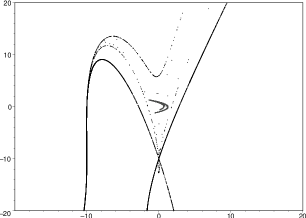
Figure 4: Phase portrait of $H_{d}^{-1}$ for $a=1.4,b=0.3,c=0.1$, together with the strange attractor for $H_{d}$.

Remark: Instead of the birational deformation of Hénon map (26), we may consider the deformation

$$\tilde{U}:\,\,\quad(u,v)\quad\,\,\longrightarrow\,\,\quad\Bigl{(}{\frac{u}{1+cu}},\,\,{\frac{v}{1+cv}}\Bigr{)},$$ (31)

for which the deformed birational mapping $H\cdot\tilde{U}$ will have a third real fixed point. Here also, the birational mapping has a “long” post-critical set in the forward direction and a “short” PC in the backward direction. We still have a continuous deformation of the strange attractor and phase portraits very similar to those shown in Fig. 1 and Fig. 2 when the input point is in the bassin of attraction. For the input out of this bassin of attraction, the iterates are attracted to the third fixed point, i.e. there are no divergent (or unbounded) orbits. We may note that this third fixed point of $H\cdot\tilde{U}$ goes to infinity for $c=\,0$ (recall that for $c=\,0$, one recovers the original bi-polynomial Hénon map).

In this example strange attractor points and points of the post-critical set cannot overlap. That is very clear in the $c\,\rightarrow\,0$ limit: points like $(0,\,-1/c)$ or $(-1/c,\,0)$ are quite naturally in the bassin of attraction of the super-attracting point at infinity of the Hénon mapping.

4 A birational mapping: $K$

To build a birational mapping $K$, we consider a combination of the Cremona inverse

$$j:\,\,\quad(x,\,y,\,z)\,\quad\,\,\longrightarrow\,\,\,\,\quad\Bigl{(}yz,\,\,xz,\,\,xy\Bigr{)},$$ (32)

and the linear transformation

$$C:\,\,\,\quad(x,\,y,\,z)\quad\,\,\longrightarrow\,\,\,\,\quad\Bigl{(}y\,+b\,z,\,z,\,x\Bigr{)},$$ (33)

giving

$$K=\,C\cdot j:\,\,\quad(x,\,y,\,z)\quad\,\,\longrightarrow\,\,\,\,\quad\Bigl{(}(z\,+b\,y)\cdot x,\,\,xy,\,\,yz\Bigr{)}.$$ (34)

In the inhomogeneous variables $u=\,x/z$, $v=\,y/z$, the birational mapping becomes

$$K:\,\,\quad(u,v)\quad\,\,\longrightarrow\,\,\quad\Bigl{(}{\frac{u}{v}}\,+\,b\,u,\,\,u\Bigr{)},$$ (35)

with inverse

$$K^{-1}:\,\,\quad(u,v)\quad\,\,\longrightarrow\,\,\quad\quad\Bigl{(}v,\,-{\frac{v}{b\,v\,-u}}\Bigr{)},$$ (36)

the linear transformation (33) becoming the collineation $(u,v)\,\rightarrow\,((b+v)/u,\,1/u)$.

The Jacobians are variables dependent and read

$$J[K]\,=\,\,\,{\frac{u}{v^{2}}},\quad\quad\quad J[K^{-1}]\,=\,\,\,{\frac{v}{(b\,v\,-u)^{2}}}.$$ (37)

The indeterminacy set and the exceptional locus, for the birational mapping $K$, are

$${\cal I}(K)\,=\,\,\,\left\{(0,\,0);\,\,\,\Bigl{(}\infty,-{{1}\over{b}}\Bigr{)}\right\},$$ (38)

$${\cal E}(K)\,=\,\,\,\,\,\left\{(u=0);\,\,(v=0)\right\}$$ (39)

and read for mapping $K^{-1}$:

$${\cal I}(K^{-1})\,\,=\,\,\,\left\{(0,\,0);\,\,(\infty,\,\infty)\right\},$$ (40)

$${\cal E}(K^{-1})\,=\,\,\,\,\,\left\{(u=bv);\,\,(v=0)\right\}.$$ (41)

The post critical set is the image by $K$ of the exceptional set:

$$K(u=0)\quad\longrightarrow\quad(0,\,0)\quad\longrightarrow\quad(\infty,\,0)\quad\longrightarrow\quad(\infty,\,\infty),$$

$$K(v=0)\quad\longrightarrow\quad(\infty,u)\quad\longrightarrow\quad(\infty,\,\infty).$$

Here also, the orbit of the critical set $K^{n}\left({\cal E}(K)\right)$ is “short”. By Diller-Favre criterion [1], only $b=\,0$ yields a complexity reduction, otherwise the mapping is “asymptotically stable” (terminology introduced in [1]). At the value $b=\,0$, the whole plane becomes a fixed point of order six which is easily seen from transformations (32), (33) which are, respectively, of order two and three. The fixed points of order one $(1,1)$, order two $(-1/2\mp i\,\sqrt{3}/2,\,\,-1/2\pm i\,\sqrt{3}/2)$ and of order three, $(1,\,-1)$, $(-1,\,-1)$ and $(-1,\,1)$ are still existing, but any deviation from these exact values throws the trajectory in the fixed point of order six.

To calculate the topological entropy [15] for the birational mapping (35), one counts the number of primitive cycles of order $\,n$, for the generic case $b\neq 0$. They are

$$\#{\rm fix}(K^{n})\,\,=\,\,\,\,[1,\,1,\,1,\,0,\,1,\,0,\,1,\,1,\,1,\,1,\,2,\,2,\,3,\,3,\,4,\,5,\,\cdots\,],$$ (42)

from which we infer the (rational) dynamical zeta function $\zeta(t)$:

$$\zeta(t)\,=\,\,\,\,{{1}\over{(1-t)\left(1-t^{2}-t^{3}\right)}}.$$ (43)

The absolute value of the inverse of the smallest root of $1-t^{2}-t^{3}=\,0$ gives the (exponential of the) topological entropy $h=\,1.324717\,\cdots$ This algebraic number is the smallest Pisot number [39, 40, 41].

When one considers mapping (35) (in the homogeneous coordinates), the growth rate of the degrees of $x$ (or $y$ or $z$) is given by the generating function

$$g(t)\,\,=\,\,\,\,{\frac{(2+2t+t^{2})\cdot t}{1-t^{2}-t^{3}}},$$ (44)

and the degree growth complexity (absolute value of inverse of smallest root of the denominator) gives again the smallest Pisot number $\lambda=\,1.324717\,\cdots\,$ This degree growth rate has been proven in [32] (and as a limiting case in [42]).

We thus see, for this mapping (and similarly to the results obtained for other transformations previously studied [9, 10, 14, 16]), an identification between the growth rate of the number of fixed points of $\,K^{n}$ and the growth rate of the degree [11, 21] of the iteration.

Following this criterion ($\lambda>1$, $h>1$), the birational mapping $K$ is chaotic. However, this criterion does not describe properly the dynamics of the mapping seen as a transformation in the real plane. It is based on the counting of degrees or fixed points irrespective of their stability.

The fixed point of order one is real for any real value of $b$. For $b=\,1$, it identifies with the fixed point at infinity. For the mapping $K$, the fixed point of order one is an unstable spiraling point for $b\,<\,0$, a stable spiraling for $0\,<b\,<\,3/4$, a stable node for $3/4\,<\,b<\,1$, a saddle for $1<\,b\,<\,3$ and an unstable node for $b\,>\,3$. The fixed point of order 2 is real and saddle for $b<-1$ and for $b\,>\,3$. It fuses with the fixed point of order one at $b=\,3$ and with the ”infinity” fixed point of order one at $b=\,-1$. The fixed point of order three is real and saddle for any real $b$.

Note that, similarly to the mapping $H_{d}^{-1}$, the backward birational mapping $K^{-1}$ has a “long” post-critical set. The iterates of the critical set has also an exponential degree growth in the parameter $b$, ruling out the existence of algebraic covariant curves.

5 The birational mapping $K$: phase portraits

The phase portraits of the birational mapping $K$ show that for $|b\,|>\,1$ the iterates are attracted to the fixed point at infinity. For $0\,<b\,<1$, the fixed point of $K$ is an attractor. For $-1<b<0$, the mapping is an attracting set. We show in Fig. 5, the attractor obtained for the value $b=\,-3/5$. This structure is independent of the initial starting points of the iteration and looks very much like a set of curves, a foliation of the $\,(u,\,v)$-plane. The structure shown in Fig. 5 is obtained from one starting point.

Figure 5: Phase portrait in the variables $(u,v)$ for $b=\,-3/5$.

Figure 6: Phase portrait in the variables $(\theta_{u},\theta_{v})$ for $b=\,-3/5$. The open circle shows the fixed point of order one.

This accumulation of curves has unbounded branches. A way to “see the global picture” amounts to performing the plot in the variables [10] $\,\theta_{u}\,=\,\arctan(u)$ and $\,\theta_{v}\,=\,\arctan(v)$. This way, the real plane is compactified to the box $\,[-\pi/2,\,\pi/2]\times[-\pi/2,\,\pi/2]$. Figure 6 shows the phase portrait in the variables $(\theta_{u},\theta_{v})$. The unbounded branches of Fig. 5 appear in Fig.6 at the bunches $(\theta_{u}=\pm\pi/2,\,\theta_{v}=\,\mp\pi/2)$ and $(\theta_{u}=\pm\pi/2,\,\theta_{v}=\,\theta_{\tilde{v}})$, the larger interval for $\,\tilde{v}$ being $[b-1,\,b]$. The attractor is thus not confined. This is consistent with the fact that it is obtained for any initial point, the basin of attraction being the whole plane.

Since the birational mapping $K$ is not integrable according to the criterion $\lambda>1$ or $h>1$, one may ask whether the structures, shown in Fig.5 and Fig.6, are compatible with a preserved meromorphic two-form or simply with covariant curves. In fact the post critical set is “short”, and there is no algebraic covariant curve. In the following, we show another way to be convinced on this non occurrence.

5.1 Non-standard fixed points

Denoting by $\,(u^{(n)},\,v^{(n)})$, the image of a point $(u,\,v)$, by transformation $\,K^{n}$, the preservation of a two-form $m(u,v)$ means:

$${{du\cdot dv}\over{m(u,\,v)}}\,\,\,=\,\,\,\,\,\,{{du^{(n)}\cdot dv^{(n)}}\over{m(u^{(n)},\,v^{(n)})}}.$$ (45)

If $J[K^{n}](u,\,v)$ denotes the Jacobian of $\,K^{n}$, one has:

$$J[K^{n}](u,\,v)\,\,=\,\,\,\,\,{{m(u^{(n)},\,v^{(n)})}\over{m(u,\,v)}}\,\,=\,\,\,\,\,{{m(K^{n}(u,\,v))}\over{m(u,\,v)}}.$$ (46)

When evaluated at the fixed point $(u_{f},\,v_{f})$ of $\,K^{n}$, the Jacobian of $\,K^{n}$ is thus equal to +1. This is what was obtained for many birational transformations we have studied [9, 15, 16]. For some of these mappings, we evaluated precisely a large number of $n$-cycles in order to get the dynamical zeta function [15, 16]. For all these mappings, a preserved meromorphic two-form exists. However, we claimed for the mapping given in [10], the non existence of a preserved meromorphic two-form since the Jacobians evaluated at (a growing number of) the fixed points of $K^{n}$ are no longer equal to one. This mapping preserves a meromorphic two-form in some subspaces of the parameters, and we showed, in this case, that the equality $J[K^{n}](u_{f},\,v_{f})=\,1$ always holds, exception of a finite number of fixed points. Thus, even when a meromorphic two-form is preserved, the equality $J[K^{n}](u_{f},\,v_{f})=\,1$ may be ruled out for the fixed points of $\,K^{n}$ that correspond to divisors of the two-form. Such “non-standard” fixed points of $\,K^{n}$ are such that $\,m(u_{f},\,v_{f})\,=\,\,0$ (or $\,m(u_{f},\,v_{f})\,=\,\,\infty$).

The number of these “non-standard” fixed points [10] of $\,K^{n}$ is an indication of the degree of $m(u,v)$, if the latter exists. When the number of such non-standard fixed points becomes very large (infinite), the existence of this algebraic two-form may be ruled out.

Thanks to the simplicity of the mappings of this paper, the expressions of these Jacobians evaluated at the fixed points may be obtained up to a large order. For instance, at respectively the order $n=\,1$, $n=\,3$, $n=\,10$ and $n=\,11$, they read ($(u_{f},v_{f})$ are the primitive fixed points of $K^{n}$)

$$J[K]\left(u_{f},v_{f}\right)\,=\,\,1-b,\quad\quad\,\,\,J[K^{3}]\left(u_{f},v_{f}\right)\,=\,\,1+b+b^{2},$$

$$J[K^{10}]\left(u_{f},v_{f}\right)\,=\,\,{\frac{(1-b^{10})\,b^{10}}{(1+b)\cdot(1-b^{5})\cdot P_{1}^{(10)}}},$$ (47)

$$J[K^{11}]\left(u_{f},v_{f}\right):\,\quad\,\,\,\,\,P_{2}^{(11)}\cdot J^{2}\,+P_{1}^{(11)}\cdot J+P_{0}^{(11)}\,=\,\,0,$$

with:

$$P_{1}^{(10)}\,=\,\,b^{8}\,-4b^{7}\,+9b^{6}\,-15b^{5}\,+16b^{4}\,-14b^{3}\,+8b^{2}\,-3b\,+1,$$

$$P_{2}^{(11)}\,=\,\,\Bigl{(}-2+8\,b-22\,{b}^{2}+46\,{b}^{3}-72\,{b}^{4}+89\,{b}^{5}-87\,b^{6}+68\,{b}^{7}$$

$$\qquad\qquad-41\,{b}^{8}+19\,{b}^{9}-6\,{b}^{10}+{b}^{11}\Bigr{)}\cdot b,$$

$$P_{1}^{(11)}\,=\,\,\,1-b+5\,{b}^{2}-2\,{b}^{3}+8\,{b}^{4}-8\,{b}^{5}+14\,{b}^{6}-25\,{b}^{7}+16\,{b}^{8}$$

$$\qquad-35\,{b}^{9}+13\,{b}^{10}-38\,{b}^{11}+21\,{b}^{12}-34\,{b}^{13}+22\,{b}^{14}-19\,{b}^{15}$$

$$\qquad+10\,{b}^{16}-5\,{b}^{17}+2\,{b}^{18}-{b}^{19},$$

$$P_{0}^{(11)}\,=\,\,\,(1-b^{11})\,\,b^{15}/(1-b).$$

As far as the fixed points up to order eleven are sufficient to make a conclusion, there is no value of the parameter $b$ that gives $J[K^{n}]$ equal to unity for these fixed points. Considering only these fixed points, a preserved meromorphic two-form for the birational mapping $K$ should be, at least, of degree $134$. In fact the proliferation of these non-standard fixed points gives a firm indication on the non existence of a preserved meromorphic two-form.

6 The birational mapping $K$: ergodic (probabilistic) analysis

While the ”complexity spectrum” of the mapping in [10] is involved (see Figure 1 in [10]), the mapping of this paper presents the same degree-growth complexity or (exponential of the) topological entropy ($\lambda=\,h=\,1.324717\cdots$) for any value of the parameter $b\neq 0$. Numerical investigation shows that the fixed points, up to the order $n=\,15$, are real for real values of the parameter $b$. We expect, then, to provide a clearer picture on the ergodic aspect of the analysis. We have seen [10] that the existence, or non existence, of preserved meromorphic two-forms has (paradoxically) no impact on the topological complexity but drastic consequences on the numerical computation of the Lyapunov exponents.

If we believe the analysis of [10], the Lyapunov exponents should be zero in the case of a preserved meromorphic two-form. This is then another check on whether the structure shown in Fig. 6 correspond to a preserved meromorphic two-form. We have computed the Lyapunov exponents for the mapping $K$ for the large values of $n$ as

$$\sigma_{1}\,=\,\,{1\over n}\,\ln\left(|\lambda_{1}|\right),\qquad\sigma_{2}\,=\,\,{1\over n}\,\ln\left(|\lambda_{2}|\right),\qquad$$ (48)

where $\lambda_{1,2}$ are the eigenvalues of

$$M^{(n)}\,=\,\,\,\,M(u^{(n-1)},\,v^{(n-1)})\,\,\,\,\cdots\,\,\,\,M(u^{(1)},\,\,v^{(1)})\,\cdot\,M(u,\,v),$$ (49)

$M$ being the tangent map evaluated at each point $\left(u^{(n)},v^{(n)}\right)$ $=\,K^{n}\left(u,v\right)$.

The Lyapunov exponents for $b\in]-1,\,0[$ are shown in Fig. 7. The largest Lyapunov exponent being positive, the attractor is chaotic.

Figure 7: Positive and negative Lyapunov exponents versus the parameter $b$

Kaplan and Yorke [43] have conjectured that the dimension of an attractor can be approximated from the spectrum of Lyapunov exponents. Essentially, this conjecture corresponds to plotting the sum of Lyapunov exponents versus $n$ (the number of Lyapunov exponents, i.e. the dimension of the system), the dimension being established by finding where the curve intercepts the $n-$axis by linear interpolation. For a two-dimensional mapping, this gives

$$D_{KY}\,=\,\,\,\,1\,\,-{\frac{\sigma_{1}}{\sigma_{2}}}$$ (50)

where $\sigma_{1}$ and $\sigma_{2}$ are respectively, the positive and negative Lyapunov exponents. This dimension is expected to be close to other dimensions such as box-counting, information and correlation dimension [45] for typical strange attractors. Kaplan-Yorke dimension (also called Lyapunov dimension) has been shown to identify with the information dimension for Baker’s transformation. It has been tested for Hénon mapping [46].

Using Kaplan-Yorke conjecture, we can compute the (fractal) dimension of the attractor which is shown in Fig.8. For $b\in\,]-1,\,0[$ the dimension of the attractor corresponds to fractals. The attractor is thus a strange attractor.

Figure 8: Kaplan-Yorke (or Lyapunov) dimension versus the parameter $b$

The dimension obtained from the Lyapunov exponents is given from a conjecture. To be more convincing on the fractal nature of the attractor, we have calculated the (fractal) dimension by the box-counting method for some values of $b$. Box-counting dimension is believed to coincide, for most systems, with Hausdorf-Besicovitch dimension. The box-counting dimension amounts to considering boxes of side $\epsilon$ covering the attractor, then counting the number of boxes $N(\epsilon)$ necessary to contain all the points. The box-counting dimension is the limit as $\,\epsilon\,\rightarrow\,0\,$ of

$$D_{box}\,=\,\,\,\,-{\frac{\ln\left(N(\epsilon)\right)}{\ln(\epsilon)}}.$$ (51)

The calculations are carried out in the variables $\theta_{u}$,  $\theta_{v}$ (which are in one-to-one correspondence with $u,\,v$). The results given in Table 1, show an agreement with the dimension computed from the Lyapunov exponents as far as the fractal nature is concerned. Note that for this mapping, the Lyapunov (Kaplan-Yorke) dimension is less than the box-counting dimension (and is a lower bound [43]).

$b$	-0.9	-0.8	-0.6	-0.5	-0.4	-0.3	-0.2
$D_{KY}$	1.17	1.24	1.37	1.42	1.47	1.51	1.57
$D_{box}$	1.34	1.36	1.44	1.52	1.52	1.56	1.66

Table 1: Kaplan-York and Box-counting dimensions for some values of the parameter $b$

Remark: The simplicity of the birational mapping $K$ makes it a good working example of many tests. For instance, it will be straightforward to compute the Lyapunov exponents and the fractal dimension from the knowledge of the first fixed points [47]. How many fixed points will be needed for that purpose? Are the fixed points sufficient to completely characterize the mapping in some ergodic analysis?

7 Conclusion

In this paper we have, first, considered four birational mappings. Three of them ($K_{1}$, $K_{2}$, $K_{4}$) have been already analyzed in previous papers and the fourth mapping ($K_{3}$) is taken from the literature on strongly regular graphs [37]. For these mappings, we have considered their post critical set versus the occurrence of covariant curves and preserved meromorphic two-form. In these working examples, the post-critical set is “long” in both directions (forwards and backwards). We have shown that the knowledge of the orbits of the critical set allows to obtain the algebraic covariant curves.

We have built a birational deformation of the Hénon map, $H_{d}$, having a “short” post-critical set. This birational mapping shows a continuous deformation of the original Hénon strange attractor. For the values of the parameters (giving a strange attractor for $H_{d}$), the backward mapping $H_{d}^{-1}$ shows an unbounded attracting set contrary to the backward Hénon map that gives divergent orbits.

We have focused on a birational mapping $K$ (slight modification of a birational mapping of Bedford and Kim [32]) which has also a “short” post-critical set, with probably no preserved meromorphic two-forms (in view of the non standard fixed points). The mapping shows an attracting set, which passes the tests of being a strange attractor.

In view of these examples, we saw that birational mappings with “short” post-critical set had no covariant curves. We also saw that strange attractors may occur for birational mappings with “short” post-critical set and they are not necessarily confined.

Appendix A The birational mapping $K_{3}$

We consider a $\,3\times 3\,$ matrix, acting on the three homogeneous variables $\,(x,\,y,\,z)\,$, taken from the analyzis of strongly regular graphs [37] matrix

$$M\,=\,\,\left[\begin{array}[]{ccc}2&a&b\\ 2&-1+c&-1-c\\ 2&-1-d&-1+d\end{array}\right],$$ (52)

and the associated collineation $\,C$. denoting $j$ the Cremona inverse (32), the mapping $K_{3}=\,C^{-1}\cdot j\cdot C\cdot j$ depends on four parameters. Here we fix $a=\,6,\,b=\,6,\,d=\,c$. The birational mapping in the variables $u=\,x/z$, $v=\,y/z$ is given by (14). The Jacobian reads:

$$J[K_{3}](u,\,v)\,=\,\,\,\,-\,5488\,{\frac{v\,N_{uv}}{u^{2}\,D_{uv}^{3}}}\cdot\left((c+1)\,uv\,-(c-1)\,u\,-2v\right)\,$$

$$\qquad\qquad\times\,((c-1)\cdot uv\,\,-(c+1)\,u\,\,+2v).$$ (53)

The exceptional varieties of the mapping are:

$${\cal E}(K_{3})\,=\,\,\,\left\{V_{1},\,V_{2},\,V_{3},\,V_{4},\,V_{5},\,V_{6}\right\}$$

$$\qquad=\left\{\begin{array}[]{ll}(u=0);\,\,(v=\,{-3u\over 1+3u});\,(v=0);\,\,(v=\,{\frac{u(c+1)}{cu-u+2}});\\ (v\,=\,\,{\frac{u(c-1)}{cu+u-2}});\,\,\,\,(D_{uv}\,=\,\,0)\end{array}\right\}.$$ (55)

The post critical set for $V_{1}$ is variable dependent. The orbit for $V_{3}$ reads

$$K_{3}^{n}(V_{3})\,=\,\,\,\,\Bigl{(}{1\over 2}\left(1+(-1)^{n}\right)\,\,+{1\over 2}\left(1-(-1)^{n}\right)\,v_{n},\,\,\,v_{n}\Bigr{)},\quad$$

$$\qquad v_{n}\,=\,\,\,\,{\frac{f(c)-f(-c)}{g(c)-g(-c)}},$$

$$f(c)\,=\,\,\,(c-7)\cdot\left(c-21\,\,-(-1)^{n}(3c-7)\right)\cdot(c+1)^{n},$$

$$g(c)\,=\,\,\,(c-7)\cdot\left(c+21\,\,-(-1)^{n}(3c+7)\right)\cdot(c-1)^{n}.$$

The orbit for $V_{2}$, after $(1,\,1)\rightarrow(\infty,\,\infty)$, gives similar expression as $V_{3}$ and reads ($n\geq 3$):

$$K_{3}^{n}(V_{2})\,=\,\,\,\Bigl{(}{1\over 2}\left(1-(-1)^{n}\right)+{1\over 2}\left(1+(-1)^{n}\right)\,v_{n},\,\,v_{n}\Bigr{)},\quad$$

$$\qquad v_{n}=\,\,\,{\frac{f(c)+f(-c)}{g(c)+g(-c)}},$$

$$f(c)\,=\,\,(c-7)\cdot\left(3c+71\,\,+(-1)^{n}(c+21)\right)\cdot(c+1)^{n-2},$$

$$g(c)\,=\,\,\,(c-7)\cdot\left(3c-7\,\,+(-1)^{n}(c-21)\right)\cdot(c-1)^{n-2}.$$

The orbit for $V_{5}$ is identical, with the change $c\,\rightarrow\,-c$, with the orbit for $V_{4}$ which reads:

$$K_{3}^{n}(V_{4})\,=\,\,\,\Bigl{(}{\frac{(c-1)(c+7)^{n}\,-(c+1)(c-7)^{n}}{f(c)\cdot v_{n}\,+(-1)^{n}\,f(-c)}}\cdot v_{n},\,\,v_{n}\Bigr{)},$$

$$\qquad v_{n}\,=\,\,\,{1\,\,\over 2}\left(1-(-1)^{n}\right)\cdot{c+7\over c-7}\,\,+{1\over 2}\left(1+(-1)^{n}\right)\cdot{c-7\over c+7},$$

$$f(c)\,=\,\,(c-1)\cdot(c+(-1)^{n}\,7)\cdot(c+7)^{n-1}.$$

Finally, the post critical set $K_{3}^{n}(V_{6})$ reads (after $(\infty,\infty)$, this is identical to $K_{3}^{n}(V_{3})$ with $c\,\rightarrow\,-c$ and a shift in $n$):

$$K_{3}^{n}(V_{6})\,=\,\,\,\Bigl{(}{1\over 2}\,(1+(-1)^{n})\,\,\,+{1\over 2}\left(1-(-1)^{n}\right)\cdot v_{n},\,\,v_{n}\Bigr{)},\quad$$

$$\quad\quad v_{n}\,=\,\,\,\,{\frac{f(c)\,-f(-c)}{f(c)\,g(c)\,\,-f(-c)\,g(-c)}},$$

$$f(c)\,=\,\,(c-7)\cdot\left(3c+7+(c+21)(-1)^{n}\right)\cdot(c+1)^{n+1},$$

$$g(c)\,=\,\,{1\over 2}\,(1-(-1)^{n})\cdot{c+7\over c-7}\,\,\,+{1\over 2}\,(1+(-1)^{n})\cdot{c-7\over c+7},$$

From these orbits, one finds easily the covariant curves. The post critical set of $K_{3}^{n}(V_{3})$ gives $u=\,1$ for $n$ even and $v=\,u$ for $n$ odd, the covariant curve is thus $(u-1)(v-u)=\,0$. The post critical set of $K_{3}^{n}(V_{4})$ gives $v\,-(c-7)/(c+7)=\,0$ for $n$ even and $v\,-(c+7)/(c-7)=\,0$ for $n$ odd, leading to the covariant curve $C_{2}=\,\left((c+7)\cdot v\,-c+7\right)\,\left((c-7)\cdot v\,-c-7\right)=\,0$. The post critical set of $K_{3}^{n}(V_{6})$ gives the same covariant curve as $K_{3}^{n}(V_{3})$.

These curves are covariant but, alone, they do not construct a preserved meromorphic two-form (see (8)). One obtains:

$$m(u,v)\,=\,\,(u-1)\,(v-u)\cdot((c+7)\,v\,-c+7)\cdot\left((c-7)\,v\,-c-7\right),$$

$${\frac{m(u^{\prime},v^{\prime})}{m(u,v)}}\,=\,\,\,\,28\,\,{\frac{N_{uv}}{D_{uv}}}\cdot J[K_{3}](u,\,v).$$

At this point, the mapping $K_{3}$ does not seem to have a preserved meromorphic two-form.

However, if a meromorphic two-form exists, we know [10] that the fixed points of the mapping for which the Jacobian is $J\,\neq\,1$ should be located on a covariant curve corresponding to the meromorphic two-form. For this mapping, there are four fixed points of order one where $J\,=\,1$ and two fixed points of order one where $J\,\neq\,1$. The latter read $(u=\,-5/2\pm\sqrt{21}/2,\,v=\,1)$ and are neither on $(u-1)(v-u)=\,0$ nor on $C_{2}=\,0$. The line $v-1=\,0$ should be covariant as this appears clearly from the expression (2.3) of the birational mapping $K_{3}$.

Producing this line $v-1=\,0$ from the iterates of $V_{1}$ may call for a tricky analysis. Instead, and since this is equivalent, we consider the backward mapping and its “long” post critical set. Cancelling the Jacobian (or its inverse) of $K_{3}^{-1}$, one obtains (among others) the algebraic curve:

$$28\,{u}^{2}\,+56\,\left(1+v\right)\,u\,-\left({c}^{2}+35\right)\,v^{2}\,+2\,({c}^{2}-35)\,v\,\,-{c}^{2}\,-35\,=\,\,0.$$

Eliminating the variable $u$ between this curve and the iterates $K_{3}^{-n}(u,v)$, will give the line $v-1=\,0$ common to both components.

Combining the covariant curves $(u-1)(v-u)=\,0$, $C_{2}=\,0$ and the new line $v-1=\,0$, one obtains

$$m_{3}(u,v)\,=\,\,\,\,{\frac{(u-1)(v-u)\cdot}{v-1}}\cdot\left((c+7)\,v\,-c+7\right)\,\left((c-7)\,v\,-c-7\right),$$

$${\frac{m_{3}(u^{\prime},v^{\prime})}{m_{3}(u,v)}}\,\,=\,\,\,\,J[K_{3}](u,\,v).$$

giving the corresponding meromorphic two-form $du\,dv/m_{3}(u,\,v)$.

Appendix B Another birational mapping: $K_{5}$

We consider the collineation $C$ corresponding to matrix (52) but with the mapping constructed as $K_{5}\,=\,\,C\cdot j$. This mapping arises in [48] and was considered in [2, 49]. For the values of the parameters $a=\,b=\,-1+q^{2}$, $c=\,d=\,q$, it was shown [48] that it has an algebraic invariant for all values of the parameter $q$. Here, we take the parameters as $a=\,b=\,q^{2}$, $c=\,d=\,q$ and the birational mapping is non integrable for generic values of $q$. The birational mapping reads

$$K_{5}:\,\,\quad(u,v)\quad\,\,\longrightarrow\,\,\qquad(u^{\prime},v^{\prime})\,=\,\,$$

$$\quad\quad\qquad\,=\,\,\,\Bigl{(}{\frac{q^{2}\cdot(1+v)\,u+2v}{D_{uv}}},\,\,\,1-{\frac{2q\cdot(v-1)\,u}{D_{uv}}}\Bigr{)},$$ (56)

$$D_{uv}\,=\,\,\,(q-1)\cdot uv\,\,-(q+1)\cdot u\,+2v,$$

with Jacobian:

$$J[K_{5}](u,\,v)\,=\,\,\,\,-8\,(1\,+q^{2})\cdot q\cdot{\frac{uv}{D_{uv}^{3}}}.$$ (57)

Its critical set reads

$${\cal E}(K_{5})\,=\,\,\,\,\left\{V_{1},\,V_{2},\,V_{3}\right\}\,\,=\,\,\,\,\left\{(v=0);\,\,(D_{uv}=0);\,\,(u=0)\right\},$$ (58)

and the first iterates of the critical set are given by

$$K_{5}^{n}(V_{1})\,=\,\,\Bigl{(}-{\frac{q^{2}}{q+1}},\,{\frac{1-q}{q+1}}\Bigr{)}\qquad\longrightarrow\qquad\Bigl{(}{\frac{1-q^{2}-q^{4}}{1+q^{4}}},\,{\frac{1-q^{4}}{1+q^{4}}}\Bigr{)},$$

$$K_{5}^{n}(V_{2})\,=\,\,(\infty,\infty)\,\,\,\rightarrow\,\,\,\Bigl{(}{\frac{q^{2}}{q-1}},\,{\frac{1+q}{1-q}}\Bigr{)}\,\,\,\rightarrow\,\,\,\Bigl{(}{\frac{1-q^{2}-q^{4}}{1-q^{4}}},\,{\frac{1+q^{4}}{1-q^{4}}}\Bigr{)}.$$

Those of $K_{5}^{n}(V_{3})$ are the same as $K_{5}^{n}(V_{2})$ after blowing down first on the point $(1,1)$.

The post-critical set for the backward mapping is also “long” and the orbits have similar expressions. The post-critical set, for both forward and backward mapping, is “long”. The degree growth in the parameter $q$ of the iterates of the critical set being exponential, there is no preserved meromorphic two-form. The phase portraits of this mapping show a foliation in the plane with infinity of leaves, similar to mapping analyzed in [10]. Note that, the line $v-1=\,0$ is covariant as easily seen from the expression of $K_{5}$. The phase portrait, shows however, no accumulation of points near this line.

Appendix C A parameter-free birational mapping

This mapping is taken from [35] and originates from lattice statistical mechanics and is related to mapping $K_{1}$. It is parameter-free, non integrable and reads

$$K_{6}:\quad(u,v)\,\quad\,\longrightarrow\,\,\quad(u^{\prime},v^{\prime})\,\,=\,\,\,\,\Bigl{(}v,\,\,{\frac{1+v-uv}{uv}}\Bigr{)}.$$ (59)

Its Jacobian reads:

$$J[K_{6}]\,\,=\,\,\,\,\,{\frac{1+v}{u^{2}v}}.$$ (60)

The orbits of the critical set read:

$$K_{6}^{n}(v=-1)\,=\,\,\,(-1,\,-1)\quad\longrightarrow\quad\left(-1,\,-1\right),$$

$$K_{6}^{n}(u=0)\,=\,\,(v,\,\infty)\rightarrow(\infty,\,(1-v)/v)\rightarrow((1-v)/v,\,-1)\rightarrow(-1,\,-1),$$

$$K_{6}^{n}(v=0)\,=\,\,(0,\infty)\quad\rightarrow\quad(\infty,\,\infty)\quad\rightarrow\quad(\infty,\,-1)\quad\rightarrow\quad(-1,\,-1).$$

The post-critical set is “short” and there is an attracting set which is the point $(-1,\,-1)$.

For the backward mapping, the orbits of the critical are

$$K_{6}^{-n}(u=-1)=\,(0,\,-1)\quad\rightarrow\quad(\infty,\,0)\quad\rightarrow\quad(1,\,\infty)\quad\rightarrow\quad(0,\,1),$$

$$K_{6}^{-n}(u=0)=\,(\infty,\,0)\quad\rightarrow\quad(1,\infty)\quad\rightarrow\quad(0,\,1)\quad\rightarrow\quad(\infty,\,0),$$

$$K_{6}^{-n}(v=-1)=\,(\infty,\,u)\quad\rightarrow\quad(1/(1+u),\,\infty)\quad\rightarrow\quad(0,\,1/(1+u))$$

$$\quad\quad\longrightarrow\quad(\infty,\,\,0)\quad\longrightarrow\quad(1,\,\infty)\quad\longrightarrow\quad(0,\,1).$$

The post critical set is short and there is an attracting set which is the cycle of order three, $\left(\infty,\,0\right)\rightarrow(1,\,\infty)\rightarrow\left(0,\,1\right)$.

Note that one may remark (see the form of the mapping) that $v+1=0$ is covariant for the forward mapping, but it is not covariant for the backward mapping, where it gives birth to an attracting point of order three.

The Jacobian evaluated at the successive fixed points gives the following. There is one fixed point of order one with $J=\,2$. There is no fixed point of order three. There is only one fixed point for the orders $2,\,4,\,5,\,6$ with respectively $J=\,\,2,\,2,\,-5,\,1$.

References

References

- [1] J. Diller and C. Favre, Dynamics of bimeromorphic maps of surfaces, Amer. J. Math. 123 (2001) 1135-1169
- [2] E. Bedford, K. Kim, On the degree growth of certain birational mappings in higher dimension, J. Geom. Anal. 14 (2004) 567-596; math.DS/0406621
- [3] E. Bedford, K. Kim, T. T. Truong, N. Abarenkov and J-M. Maillard, Degree Complexity of a Family of Birational Maps, Math. Phys. Anal. Geom. 11 (2008) 53-71; math.DS/0711.1186v2
- [4] C.T. McMullen, Dynamics on blowups of the projective plane, Publications Mathématiques de l’IHES, 105 (2007) 49-89
- [5] M. Hénon, A two dimensional mapping with a strange attractor, Commun. Math. Phys. 50 (1976)69
- [6] G. I. Bischi, L. Gardini and C. Mira, Plane maps with denominator. I. Some generic properties, Int. J. Bifur. Chaos 9 (1999) 119-153
- [7] G. I. Bischi, C. Mira and L. Gardini, Unbounded sets of attraction, Int. J. Bifur. Chaos 10 (2000) 1437-1469
- [8] L. Billings, J.H. Curry and E. Phipps, Lyapunov exponents, singularities, and a riddling bifurcation, Phys. Rev. Lett. 79 (1997) 1018-1021
- [9] S. Boukraa, S. Hassani and J.-M. Maillard, Noetherian mappings, Physica D 185 (2003) 3-44
- [10] M. Bouamra, S. Boukraa, S. Hassani, J.-M. Maillard, Post-critical set and non existence of preserved meromorphic two-forms, J. Phys.A 38 (2005) 7957-7988
- [11] N. Abarenkova, J-C. Anglès d’Auriac, S. Boukraa and J-M. Maillard, Growth-complexity spectrum of some discrete dynamical systems, Physica D 130 (1999) 27-42; chao-dyn/9807031
- [12] V.I. Arnold, Dynamics of complexity of intersections, Bol. Soc. Bras. Mat. 21 (1990) 1-10
- [13] V. Arnold, Problems on singularities and dynamical systems, Developments in Mathematics. The Moscow School, V. Arnold and M. Monarstyrsky editors (Chapman and Hall, London, 1993)
- [14] N. Abarenkova, J-C. Anglès d’Auriac, S. Boukraa, S. Hassani and J-M. Maillard, Real Arnold complexity versus real topological entropy for birational transformations, J. Phys A 33 (2000) 1465-1501 and chao-dyn/9906010
- [15] N. Abarenkova, J.-C. Anglès d’Auriac, S . Boukraa, S. Hassani and J.-M. Maillard, Topological entropy and Arnold complexity for two-dimensional mappings, Phys. Lett. A 262 (1999) 44-49 and chao-dyn/9806026
- [16] N. Abarenkova, J.-C. Anglès d’Auriac, S. Boukraa, S. Hassani and J.-M. Maillard, Rational dynamical zeta functions for birational transformations, Physica A 264 (1999) 264-293
- [17] N. Abarenkova, J.-C. Anglès d’Auriac, S. Boukraa and J.-M. Maillard, Real topological entropy versus metric entropy for birational measure-preserving transformations, Physica D 144 (2000) 387-433
- [18] C. Favre, Points périodiques d’applications birationnelles, Ann. Inst. Fourier (Grenoble) 48 (1998) 999-1023
- [19] M. Artin and B. Mazur, On periodic points, Ann. Math. 81 (1965) 82
- [20] S. Boukraa, J-M. Maillard and G. Rollet, Almost integrable mappings, Int. J. Mod. Phys. B 8 (1994) 137-174
- [21] S. Boukraa and J-M. Maillard, Factorization properties of birational mappings, Physica A 220 (1995) 403
- [22] I. Gumowski and C. Mira, Dynamique chaotique, (Cepadues Editions, Toulouse, 1980)
- [23] V.S. Afrajmovich, V.I. Arnold, Yu S. Il’yashenko and L.P. Shel’nikov, Dynamical systems V: Bifurcation theory and catastrophe theory, (Springer, Berlin, 1994)
- [24] S.V. Gonchenko, D.V. Turaev, P. Gaspard and G. Nicolis, Complexity in the bifurcation structure of homoclinic loops to a saddle-focus, Nonlinearity 10 (1997) 409-423
- [25] E. Bedford and J. Diller, Real and complex dynamics of a family of birational maps of the plane: the golden mean subshift, Amer. J. Math. 127 (2005) 595-646; arXiv: math.DS/0306276 v1
- [26] E. Bedford and J. Diller, Energy and invariant measures for birational surface maps, Duke Math. J. 128 (2005) 331-368, and arXiv:math.CV/0310002
- [27] J.P. Eckman and D. Ruelle, Ergodic theory of chaos and strange attractors, Rev. Mod. Phys. 57 (1985)617
- [28] V. S. Anishchenko, T. E. Vadivasova, G. I. Strelkova and A. S. Kopeikin, Chaotic attractors of two-dimensional invertible maps, Dis. Dyn. Nat. Soc. 2 (1998) 249
- [29] P. Cvitanovoc, G. H. Gunaratne and I. Procaccia, Topological and metric properties of Hénon-type strange attractors, Phys. Rev. A 38 (1988)1503-1520
- [30] D. Ruelle, What is a strange attractor?, Notices of the AMS 53 (2006) 764-765
- [31] R. Brown and L. O. Chua, Clarifying chaos: examples and counterexamples, Int. J. Bifur. Chaos 6 (1996) 219-249
- [32] E. Bedford and K. Kim, Periodicities in linear fractional recurrences: Degree growth of birational surface maps, Mich. Math. J. 54 (2006) 647-671; arXiv:math.DS/0509645
- [33] M. Csornyei and M. Laczkovich, Some periodic and non periodic recursions, Mon. Math. 132 (2001) 215-236
- [34] E. A. Grove and G. Ladas, Periodicities in nonlinear difference equations, (Kluwer Academic Publishers, 2005)
- [35] S. Boukraa, S. Hassani and J.-M. Maillard, New integrable cases of a Cremona transformation: a finite-order orbits analysis, Physica A 240 (1997) 586-621
- [36] G.R.W. Quispel and J.A.G. Roberts, Reversible mappings of the plane, Phys. Lett. A 132, (1988), pp. 161-163.
- [37] F. Jaeger, Strongly regular graphs and spin models for the Kauffman polynomial, Geom. Dedicata 44 (1992)23-52
- [38] C. Favre and M. Jonsson, The valuative tree, Lecture Notes in Math, 1853, Springer Verlag, (2004)
- [39] C. Pisot, La répartition modulo 1 et les nombres algébriques, Annali di Pisa 7,(1938) 205-248
- [40] D. W. Boyd, Pisot Numbers in the Neighbourhood of a Limit Point I, J. Number Theory 21, (1985) 17-43
- [41] M.J. Bertin, A. Decomps-Guilloux, M. Grandet-Hugot, M. Pathiaux-Delefosse and J.P; Schreiber, Pisot and Salem numbers, (Birkhauser Verlag, 1992)
- [42] S. Cantat, Dynamique des automorphismes des surfaces projectives complexes, C.R. Acad. Sci. Paris, t. 328 (1999) 901-906
- [43] J. Kaplan and J.A. Yorke, Chaotic behavior of multidimensional difference equations, in: Functional differential equations and approximations of fixed points, H.O. Peitgen and H.O. Walther (eds.), Lecture Notes in Mathematics, Vol. 730, (Springer, Berlin, 1979) pp.228-237
- [44] K.E. Chlouverakis and J.C. Sprott, A comparison of correlation and Lyapunov dimensions, Physica D 200 (2004)156
- [45] P. Grassberger and I. Procaccia, Characterization of strange attractors, Phys. Rev. Lett. 50 (1983) 346
- [46] D.A. Russel, J.D. Hansen and E. Ott, Dimension of strange attractors, Phys. Rev. Lett. 45 (1980) 1175
- [47] P. Cvitanovic, Invariant measurement of strange sets in terms of cycles, Phys. Rev. Lett. 61 (1988) 2729-2732
- [48] M.P. Bellon, J.M. Maillard and C.M; Viallet, Integrable Coxeter groups, Phys; Lett. A 159 (1991) 221-232
- [49] C.M. Viallet, On some Coxeter groups, CRM Proceedings and Lecture Notes, Volume 9 (1996) 377-388