Observed Universality of Phase Transitions in High-Dimensional Geometry, with Implications for Modern Data Analysis and Signal Processing

Abstract.

We review connections between phase transitions in high-dimensional combinatorial geometry and phase transitions occurring in modern high-dimensional data analysis and signal processing. In data analysis, such transitions arise as abrupt breakdown of linear model selection, robust data fitting or compressed sensing reconstructions, when the complexity of the model or the number of outliers increases beyond a threshold. In combinatorial geometry these transitions appear as abrupt changes in the properties of face counts of convex polytopes when the dimensions are varied. The thresholds in these very different problems appear in the same critical locations after appropriate calibration of variables.

These thresholds are important in each subject area: for linear modelling, they place hard limits on the degree to which the now-ubiquitous high-throughput data analysis can be successful; for robustness, they place hard limits on the degree to which standard robust fitting methods can tolerate outliers before breaking down; for compressed sensing, they define the sharp boundary of the undersampling/sparsity tradeoff curve in undersampling theorems.

Existing derivations of phase transitions in combinatorial geometry assume the underlying matrices have independent and identically distributed (iid) Gaussian elements. In applications, however, it often seems that Gaussianity is not required. We conducted an extensive computational experiment and formal inferential analysis to test the hypothesis that these phase transitions are universal across a range of underlying matrix ensembles. We ran millions of linear programs using random matrices spanning several matrix ensembles and problem sizes; to the naked eye, the empirical phase transitions do not depend on the ensemble, and they agree extremely well with the asymptotic theory assuming Gaussianity. Careful statistical analysis reveals discrepancies which can be explained as transient terms, decaying with problem size. The experimental results are thus consistent with an asymptotic large-$n$ universality across matrix ensembles; finite-sample universality can be rejected.

Keywords: High-Throughput Measurements, High Dimension Low Sample Size datasets, Robust Linear Models. Compressed Sensing, Geometric Combinatorics.

1. Introduction

Recent work has exposed a phenomenon of abrupt phase transitions in high-dimensional geometry. The phase transitions amount to rapid shifts in the likelihood of a property’s occurrence when a dimension parameter crosses a critical level (a threshold). We start with a concrete example, and then identify surprising parallels in data analysis and signal processing.

1.1. Convex hulls of Gaussian point clouds

Suppose we have a sample $X_{1}$, …, $X_{n}$ of independent standard normal random variables in dimension $d$, forming a point cloud of $n$ points in $\bf R^{d}$. Our intuition suggests that a few of the points will lie on the ‘surface’ of the dataset, that is, the boundary of the convex hull; the rest will lie ‘inside’, i.e. interior to the hull. However, if $d$ is a fixed fraction of $n$ and both are large, our intuition is completely violated. Instead, all of the points are on the boundary of the convex hull – none is interior. Moreover, the line segment connecting the typical pair of points does not intersect the interior; in complete defiance of expectation, it stays on the boundary. Even more, for $k$ in some appreciable range, the typical $k$-tuple spans a convex hull which does not intersect the interior! For humans stuck all their lives in three-dimensional space, such a situation is hard to visualize.

The phenomenon of phase transition appears as follows: such seemingly strange behavior continues for quite large $k$, up to a predictable threshold given by a formula $k^{*}=d\cdot\rho(d/n;T)$, where $\rho()$ is defined in §2 below. Below this threshold (i.e. $k$ a bit smaller than $k^{*}$), the strange behavior is observed; but suddenly, above this threshold (i.e. for $k$ a bit larger) our normal low-dimension intuition works again – convex hulls of $k$-tuples of points indeed intersect the interior.

This curious phenomenon in high-dimensional geometric probability is one of a small number of fundamental such phase transitions. We claim they have consequences in several applied fields:

• in selecting models for statistical data analysis of large datasets,

• in coping with outlying measurements in designed experiments,

• in determining how many samples we need to take in designing imaging devices.

The consequences can be both profound and important. They range from negative-philosophical – if your database has too many ’junk’ variables in it nothing can be learned from it – to positive-practical – it isn’t really necessary to sit cooped up for an hour in a medical MRI scanner: with the right software, the necessary data could be collected in a fraction of the time commonly used today.

Our paper will help the reader understand more precisely what these phase transitions are and where they may occur in science and technology; it will then discuss our

Main contribution. We have observed a universality of threshold locations across a range of underlying probability distributions. We are able to change the underlying distribution from Gaussian to any one of a variety of non-Gaussian choices, and we still observe phase transitions at the same locations.

We compiled evidence based on millions of random trials and observed the same phase transitions even for several highly non-iid ensembles. We here formally state and test the universality hypothesis.

Our research leads to an intriguing challenge for high-dimensional geometric probability:

Open problem. Characterize the universality class containing the standard Gaussian: i.e. the class of matrix ensembles leading to phase transitions matching those for Gaussian polytopes.

Evidently this class is fairly broad. In view of the significance of these phase transitions in applications, this is quite an attractive challenge. We begin by illustrating three surprising appearances of these phase transitions.

1.2. First surprise: model selection with large databases

A characteristic feature of today’s data deluge is the tendency in each field to collect ever more and more measurements on each observed entity, whether it be a pixel of sky, a sample of blood or a sick patient. Technology continually puts in our hands high-throughput measurement equipment making ever more varied and ever more detailed numerical measurements on the spectrum of light, the protein expression in whole blood or fluctuations in neural or muscular activity.

As a result, observed entities are represented by ever higher-dimensional feature vectors. In fact the transition between the 20th and 21st centuries marked a sudden increase in the dimensionality of typical datasets that scientists studied, so that it became unremarkable for each observational unit to be represented as a data point in a $p$-dimensional space with $p$ very large – in the hundreds, thousand or millions.

The modern trend to high-throughput measurement devices often does not address the fundamental difficulty of obtaining good observational units. Scientists face the same troubles they always have faced when searching for subjects affected by a rare disease, or observing rare events in distant galaxies. Hence, in many fields the number of observational units stays small, perhaps in the hundreds (or even dozens), but each of those few units can now be routinely subjected to unprecedented density of numerical description.

Orthodox statistical methods assumed a quite different set of conditions: an abundance of observational units and a very limited set of measured characteristics on each unit. Modern statistical research is intensively developing new tools and theory to address the new unorthodox setting; such research comprised much of the activity in the recent 6-month Newton Institute programme Statistical Theory and Methods for Complex, High-Dimensional Data.

Consider a linear modelling scenario going back to Legendre, Gauss and perhaps even before. We have available a response variable $Y$ which we intend to model as a linear function of up to $p$ numerical predictor variables $X_{1}$, …, $X_{p}$. We contemplate an utterly standard multvariate linear model, $Y=\alpha+\sum_{j}\beta_{j}X_{j}+Z$ where the $\beta_{j}$ are regression coefficients and $Z$ is a standard normal measurement error. In words, the expected value of $Y$ given $\{X_{j}\}$ is a linear combination with coefficients $\beta_{j}$.

Suppose we have a collection of measurements $(Y_{i},X_{i,j},j=1,\dots,p)$, one for each observational unit $i$. We will use these data to estimate the $\beta_{j}$’s, allowing future predictions of $Y$ given the $X_{j}$’s.

In the ‘21st Century Setting’ described above, we have more predictor variables than observations, meaning $p>n$. While Legendre and Gauss may have understood the $p<n$ case, they would have been very troubled by the $p>n$ case: there are more unknowns than equations, and there is noise to boot!

A key feature of high-throughput analysis is that batches of potential predictors are automatically measured but one does not know in advance which, if any, may be useful in a particular project. Researchers in applied sciences where high throughput studies are popular (e.g. genomics, proteomics, metabolonomics) believe that some small fraction of the measured features are useful, among many useless ones. Unfortunately, high-throughput techniques give us everything, useful and useless, all mixed together in one batch.

In this setting, a reasonable response is forward stepwise linear regression. We proceed in stages, starting with the simple model $Y=\alpha+Z$ (i.e. no dependence on $X$’s) and at each stage expand the model by adding the single variable $X_{j}$ offering the strongest improvement in prediction.

Donoho & Stodden (2006) conducted a simulation experiment using forward stepwise regression with False-Discovery-Rate control stopping rule. Their experiment chose $p=200$ and explored a range of $n<p$ cases. Letting $k$ denote the number of useful predictors among the $p$ potential predictors, they set up true underlying regression models reflecting the choice $(k,n,p)$, ran the stepwise regression routine, and recorded the mean squared prediction error of the resulting estimate. Figure 1 displays results: the coloured attribute gives the relative mean-squared error of the estimate; the axes present the ratio $\delta=n/p$ of observations to variables, with $0<\delta<1$ in this brave new world, and $\rho=k/n$ of useful variables to observational units. Evidently there is an abrupt change in performance: one can suddenly ‘fall off a cliff’ by slightly increasing the number of useless variables per useful variable. The surprise is that the ‘cliff’ is roughly at the same position as the overlaid curve. That curve, denoted by $\rho(\delta;C)$ and defined fully below, derives from combinatorial geometry notions similar to those in §1.1.

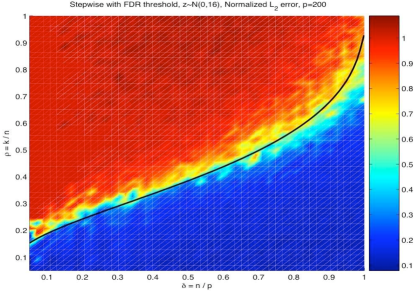
Figure 1. Phase Transition in Stepwise Regression Performance. Average fractional error of the regression coefficients from Forward Stepwise Regression with a False Discovery Threshold, $\|\hat{\beta}-\beta\|/\|\beta\|$ (Donoho & Stodden 2006). Horizontal axis: $\delta=n/p$ (number of observations/number of variables). Vertical axis $\rho=k/n$ (number of useful variables / number of observations). Solid curve $\rho(\delta;C)$ from combinatorial geometry. The rapid deterioration in performance roughly coincides with this curve

Interpretation:

• A standard scientific data analysis approach in the ‘21st century setting’ ‘falls off a cliff’, failing abruptly when the model becomes too complex.

• The location of this failure (ratio of model variables to observations) matches a curve derived from the field of geometric combinatorics!

1.3. Surprise 2: robustness in designed experiments

We now consider a problem in robust statistics. Suppose that a response variable $Y$ is thought to depend on $p$ independent variables $X_{1}$, …, $X_{p}$. Unlike the data-drenched high-throughput observational studies of §1.2 we are in a classical designed experiment, with $p<n$. The dependence is linear, so we again have $Y=\sum_{j}\beta_{j}X_{j}+Z+W$. The error $Z$ is again normal, but $W$ is a ‘wild’ variable containing occasional very large outliers.

Most scientists realize that such outliers could upset the usual least-squares procedure for estimating $\beta$, and many know that $\ell_{1}$ minimization,

(1.1) $$\min_{b}\|Y-X^{\prime}b\|_{1},$$

is purported to be ‘robust’, particularly in designed experiments where wild $X$’s do not occur. Let us focus on a specific designed experiment, where $X$ is an $n$ by $p$ partial Hadamard matrix, i.e. $p$ columns chosen at random from an $n\times n$ Hadamard matrix. This design chooses $X_{i,j}$ either $+1$ or $-1$ in a very specific way; there are no wild $X$’s. We let the outlier generators $W$ have most entries $0$, but, in our study, a small fraction $\epsilon=k/n$ – at randomly-chosen sites – will have very large values; in any one realization they can either be all large positive or all large negative.

To clarify better the relationships we are trying to make in this paper we set the standard error $Z$ to zero, and consider only the ’wild’ outliers in $W$. We quantify breakdown properties of the $\ell_{1}$ estimator by a large computational experiment. We vary parameters $(k,n,p)$ creating a range of situations. At each one, we solve the $\ell_{1}$ fitting problem (1.1) and measure to how many digits $\hat{\beta}$ agrees with $\beta$; we record $\hat{\beta}$ as breaking down due to outliers when fewer than six digits agree. Panel (a) in figure 2 shows the results of this experiment, depicting the breakdown fraction.

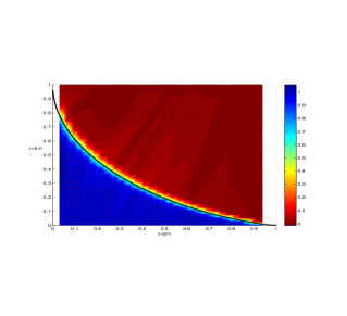
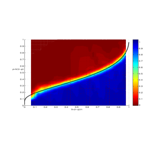
Figure 2. Breakdown Point of $\ell^{1}$ Fitting. Shaded attribute: fraction of realizations in which regression coefficients from (1.1) are accurate to within six digits. Panel (a) Horizontal axis: $\gamma=p/n$. Vertical axis: $\epsilon=k/n$. Curve: $\epsilon^{*}(\gamma)$. Panel (b) Horizontal axis: $\delta=(n-p)/n$. Vertical axis: $k/p$. Curve: $\rho(\delta;C)$. Same data underly both panels. The left panel uses variables that are natural for robustness experts; the right panel uses variables showing the agreement with the pattern already seen in figure 1.

Evidently, there is an abrupt change in behaviour at a certain critical fraction $\epsilon^{*}$; this depends on $\gamma=p/n$. Now $0<\gamma<1$, so there are here more observational units than predictors. When there are many observation units per predictor, i.e. $\epsilon^{*}\approx 1$, $\ell_{1}$ fitting can resist a large fraction of outliers. When the model is almost saturated, i.e. nearly one predictor per observation, $\epsilon^{*}\approx 0$, it takes very little contamination to break down the $\ell_{1}$ estimator. On figure 2(a) we overlay a theoretical curve $\epsilon^{*}(\gamma;C)=(1-\gamma)\rho((n-p)/n;C)$ where $\rho(\cdot;Q)$ is derived from geometric combinatorics. Evidently the curve coincides with the observed breakdown point of the $\ell_{1}$ estimator in a designed experiment. Figure 2(b) depicts a transformation of panel (a), into new axes, with variables $\rho=k/(n-p)$ and $\delta=(n-p)/n$. The display looks now similar to Stodden’s figure 1.

Interpretations:

• Standard $\ell_{1}$ fitting in a standard designed experiment (but with large $n$ and $p$, this time with $p<n$) turns out to be robust below a certain critical fraction of outliers, at which point it breaks down.

• The simulation results, properly calibrated, closely match seemingly unrelated phenomena in sparse linear modelling in the $p>n$ case.

• This critical fraction matches a known phase transition in geometric combinatorics.

1.4. Surprise 3: compressed sensing

We now leave the field of data analysis for the field of signal processing.

Since the days of Shannon, Nyquist, Whittaker and Kotelnikov, the ‘sampling theorem’ has helped engineers decide how much data need to be acquired in design of measurement equipment. Consider, therefore, the following imaging problem. We wish to acquire a signal $x_{0}$ having $N$ entries. Now suppose that only $k\ll N$ of those pixels are actually nonzero – we do not know which ones are nonzero, or even that this is true. There are $N$ degrees of freedom here, since any of the $N$ pixel values vary.

Consider making $n\ll N$ measurements of a special kind. We simply observe $n$ random Fourier coefficents of $x$. Here $n\ll N$ so that, although the image has $N$ degrees of freedom, we make far fewer measurements. Let $A$ be the linear operator that delivers the selected $n$ Fourier coefficients and let $y$ be the resulting measured coefficients. We attempt to reconstruct by solving for the object $x_{1}$ with smallest $\ell_{1}$ norm subject to agreeing with the measurements $y$:

(1.2) $$\min\|x\|_{1}\mbox{ subject to }y=Ax.$$

Figure 3 shows results of computational experiments conducted by the authors. In those experiments we chose $N=200$ and varying levels of $k$ and $n$. The horizontal axis $\delta=n/N$ measures the undersampling ratio – how many fewer measurements we are making than the customary $N$. The vertical axis $\rho=k/n$ measures to what extent the effective number of degrees of freedom $k$ is smaller than the number of measurements. The contours indicate the success rate. The superimposed curve $\rho(\delta;C)$ roughly coincides with the empirical 50% success rate curve.

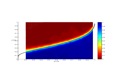
Figure 3. Compressed Sensing from random Fourier measurements. Shaded attribute: fraction of realizations in which $\ell_{1}$minimization (1.2) reconstructs an image accurate to within six digits. Horizontal axis: undersampling fraction $\delta=n/N$. Vertical axis: sparsity fraction $\rho=k/n$.

Interpretation: We can violate the usual ‘sampling theorem’ ($n\geq N$) with impunity! The true limit is $n\gtrsim k/\rho(n/N;C)$, where $\rho(\delta;C)$ is the curve decorating the display. We have seen this curve twice before already; it arises in a superficially unrelated problem in high-dimensional geometric combinatorics.

1.5. The connection to high-dimensional geometric combinatorics

Recall the problem in geometric probability we discussed in §1.1. Draw a sequence of $n$ samples $X_{1},\dots,X_{n}$ from a standard $d$-dimensional normal distribution. Let $P=Conv(X_{1},\dots X_{n})$ denote the convex hull of these $n$ points; this is a random convex polytope.

Suppose that $d$ and $n$ are both large, and let $\delta=d/n$. Figure 4 presents a black curve to be called $\rho(\delta;T)$ and formally defined in §2. It has the following interpretation.

Let $\rho=k/d$. Suppose that $\rho<\rho(d/n;T)$ and that $n$ and $d$ are both large, with $d<n$. For the typical $k+1$ tuple $(X_{i_{1}},\dots X_{i_{k+1}})$,

• every $X_{i_{j}}$ is a vertex of $P$, $1\leq j\leq k+1$;

• every line segment $[X_{i_{j}},X_{i_{j^{\prime}}}]$ is an edge of $P$, $1\leq j,j^{\prime}\leq k+1$;

• …

• the convex polytope $Conv(X_{i_{1}},\dots X_{i_{k+1}})$ is a $k$-dimensional face of $P$.

Figure 4 also presents a second, lower, black curve, which is actually the one we have seen in our three surprises. This curve, denoted by $\rho(\delta;C)$ and defined in §2, has the following interpretation. Draw the same $n$ samples $X_{1},\dots,X_{n}$ from a standard $d$-dimensional normal distribution. Now let $Q=Conv(X_{1},\dots,X_{n},-X_{1},\dots,-X_{n})$ denote the convex hull of the $2n$ points including the original $n$ points and their reflections through the origin. This is a random centrosymmetric convex polytope.

Let $\rho=k/d$ and $\epsilon>0$. Suppose that $\rho<\rho(d/n;C)(1-\epsilon)$ and that $n$ and $d$ are both large. For the typical $k+1$ tuple $(X_{i_{1}},\dots X_{i_{k+1}})$,

• every $\pm X_{i_{j}}$ is a vertex of $Q$, $1\leq j\leq k+1$;

• every line segment $[\pm X_{i_{j}},\pm X_{i_{j^{\prime}}}]$ is an edge of $Q$, $1\leq j,j^{\prime}\leq k+1$;

• …

• the typical convex polytope $Conv(\pm X_{i_{1}},\dots\pm X_{i_{k+1}})$ is a $k$-dimensional face of $Q$.

In short, the curve arising each time in Surprises 1-3 involves convex hulls of symmetrized Gaussian point clouds. The curve involving $\rho(\delta;T)$ would arise if we had instead positivity constraints on the objects to be recovered (Surprises 1 and 3) or on the outliers (Surprise 2).

1.6. This paper

The curve $\rho(\delta;C)$ describes properties of high-dimensional polytopes deriving from the Gaussian distribution. What now seems surprising about Surprises 1-3 is the lack of formal connection to those polytopes in the applications. For example

• In Surprise 1, stepwise regression as practised by statisticians seems unrelated to convex polytopes.

In Surprises 2 and 3, the appearance of the $\ell_{1}$ norm establishes a connection with convex polytopes (as the unit ball of the $\ell_{1}$ norm is in fact a regular polytope). Yet

• In Surprise 2, neither a Hadamard design nor outliers have any formal connection to any Gaussian distribution.

• In Surprise 3, observing random frequencies of the Fourier transform of a two-dimensional signal has no visible connection to any Gaussian distribution.

The curves $\rho(\delta;C)$ and $\rho(\delta;T)$ accurately describe thresholds in many situations where the Gaussian distribution is not present; in fact we have witnessed it in cases where the points of a point cloud were chosen deterministically. We believe this signals a new kind of limit theorem in probability theory that, when formalized, will make precise a new kind of universality phenomenon in high-dimensional geometry.

2. Geometric combinatorics and phase transitions

2.1. Polytope terminology

Let $P$ be a convex polytope in $\bf R^{N}$, i.e. the convex hull of points $p_{1},\dots,p_{m}$. Let $A$ be an $n\times N$ matrix. The image $Q=AP$ lives in $\bf R^{n}$; it is a convex set, in fact a polytope, the convex hull of points $Ap_{1},\dots,Ap_{m}$. $Q$ is the result of ‘projecting’ $P$ from $\bf R^{N}$ down to $\bf R^{n}$ and will be called the projected polytope.

The polytopes $P$ and $Q$ are have vertices, edges, $2$-dimensional faces, … . Let $f_{k}(P)$ and $f_{k}(Q)$ denote the the number of such $k$-dimensional faces; thus $f_{0}(P)$ is the number of vertices of $P$ and $f_{N}(P)$ the number of facets, while $f_{0}(Q)$ is the number of vertices and $f_{n}(Q)$ the number of facets. Projection can only reduce the number of faces, so

$$f_{k}(Q)=f_{k}(AP)\leq f_{k}(P),\qquad k\geq 0.$$

Three very special families of polytopes $P$ are available in every dimension $N>2$, the so-called regular polytopes. Here we consider two of the three:

• the simplex (an $(N-1)$-dimensional analogue of the equilateral triangle)

  (2.3) $$T^{N-1}:=\left\{x\in\bf R^{N}|\quad\sum_{i=1}^{N}x_{i}=1,\quad x_{i}\geq 0\right\},$$

  and the

• cross-polytope (an $N$-dimensional analogue of the octahedron)

  (2.4) $$C^{N}:=\left\{x\in\bf R^{N}|\quad\sum_{i=1}^{N}|x_{i}|\leq 1,\right\}$$

Statements concerning the hypercube similar to those made here for the simplex and cross-polytope are available to an interested reader in Donoho & Tanner (2008$a$).

2.2. Connection to underdetermined systems of equations

The regular polytopes are simple and beautiful objects, but are not commonly thought to be useful objects. However, their face counts reveal solution properties of underdetermined systems of equations. Such underdetermined systems arise frequently in modern applications and the existence of unique solutions to such systems is responsible for the three surprises given in the introduction. Consider the case of the simplex.

Consider the underdetermined system of equations $y_{0}=Ax$, where $A$ is $n\times N$, $n<N$, and the optimization problem (LP):

(LP) $$\min 1^{\prime}x\mbox{ subject to }y_{0}=Ax,\quad x\geq 0.$$

Of course, ordinarily, the system has an infinite number of solutions as does the problem (LP) .

Lemma 2.1.

Let $A$ be a fixed matrix with $n$ columns in general position in $R^{N}$. Consider vectors $y_{0}$ with a sparse solution $y_{0}=Ax_{0}$ where $x_{0}\geq 0$ has $k$ nonzeros. The fraction of systems $(y_{0},A)$ where (LP) has that underlying $x_{0}$ as its only solution is

$$fraction\{\mbox{Exact Reconstruction using (LP)\ }\}=\frac{f_{k}(AT^{N-1})}{f_{k}(T^{N-1})}.$$

In short, the ratio of face counts between the projected simplex and the unprojected simplex tells us the probability that the (LP) correctly reconstructs a $k$-sparse $x_{0}$.

Consider the case of the cross-polytope. Apply the optimization problem (P1)  to the problem instance $(y_{0},A)$ generated by

(P1) $$\min\|x\|_{1}\mbox{ subject to }y_{0}=Ax,$$

an underdetermined system of equations $y_{0}=Ax_{0}$, where $A$ is $n\times N$, $n<N$ . Of course, ordinarily, both the linear system and the problem (P1) have an infinite number of solutions.

Lemma 2.2.

Let $A$ be a fixed matrix with $n$ columns in general position in $R^{N}$. Consider vectors $y_{0}$ with a sparse solution $y_{0}=Ax_{0}$ where $x_{0}$ has $k$ nonzeros. The fraction of systems $(y_{0},A)$ where (P1) has that underlying $x_{0}$ as its unique solution is

$$fraction\{\mbox{Reconstruction using (P1)\ }\}=\frac{f_{k}(AC^{N})}{f_{k}(C^{N})}.$$

In short, the ratio of face counts between the projected cross-polytope and the unprojected cross-polytope tells us the probability that (P1) can successfully recover a true underlying $k$-sparse object.

In short, it is essential to know whether or not

$$\frac{f_{k}(AQ)}{f_{k}(Q)}\approx 1$$

for $Q$ the simplex or cross-polytope.

2.3. Asymptotics of face counts with Gaussian matrices $A$

We now consider the case where the $n$ by $N$ matrix $A$ has iid Gaussian random entries. Then the mapping $P\mapsto Q$ is a random projection. In this case, rather amazingly, tools from polytope theory and probability theory can be combined to study the expected face counts in high dimensions. The results demonstrate rigorously the existence of sharp thresholds in face count ratios.

Theorem 2.1 (Donoho (2005$a,b$), Donoho & Tanner (2005$a,b$, 2009$a$)).

Let the $n\times N$ random matrix $A$ have iid $N(0,1)$ Gaussian elements. Consider sequences of triples $(N,n,k)$ where $n=\delta N$ , $k=\rho n$, and $N\rightarrow\infty$. There are functions $\rho(\delta;Q)$ for $Q\in\{T,C\}$ demarcating phase transitions in face counts:

$$\lim_{N\rightarrow\infty}\frac{f_{k}(AQ)}{f_{k}(Q)}=\left\{\begin{array}[]{ll}1&\rho<\rho(\delta,Q)\\ 0&\rho>\rho(\delta,Q).\end{array}\right.$$

Figure 4 displays the two curves referred to in this theorem. The simplex’s transition is higher than the cross-polytope’s: $\rho(\delta,T)>\rho(\delta,C)$ for $\delta\in(0,1)$.

3. Empirical results for non-Gaussian ensembles

3.1. Explorations

Over the last few years we ran computer experiments generating millions of underdetermined systems of equations of various kinds, using standard optimization tools to select specific solutions, and checking whether or not the solution was unique and/or sparse. In overwhelmingly many cases, Gaussian polytope theory accurately matches the experimental results, even when the matrices involved are not Gaussian. We here summarize results about experiments with the non-Gaussian ensembles listed in table 1. Further detail is provided in the Electronic Materials Supplement (Donoho & Tanner 2009$b$).

Suite	Ensemble Name	Coefficients	Matrix Ensemble
3	Bernoulli	+	iid elements equally likely to be 0 or 1
4	Bernoulli	$\pm$	iid elements equally likely to be 0 or 1
5	Fourier	+	$n$ rows chosen at random from $N$ by $N$ DCT matrix
6	Fourier	$\pm$	$n$ rows chosen at random from $N$ by $N$ DCT matrix
7	Ternary (1/3)	+	iid elements equally likely to be -1, 0 or 1
8	Ternary (1/3)	$\pm$	iid elements equally likely to be -1, 0 or 1
9	Ternary (2/5)	+	iid elements taking values -1, 0 or 1 with $P(0)=3/5$
10	Ternary (2/5)	$\pm$	iid elements taking values -1, 0 or 1 with $P(0)=3/5$
11	Ternary (1/10)	+	iid elements taking values -1, 0 or 1 with $P(0)=9/10$
12	Ternary (1/10)	$\pm$	iid elements taking values -1, 0 or 1 with $P(0)=9/10$
13	Hadamard	+	$n$ rows chosen at random from $N$ by $N$ Hadamard matrix
14	Hadamard	$\pm$	$n$ rows chosen at random from $N$ by $N$ Hadamard matrix
15	Expander	+	special binary matrices, here with $P(0)=14/15$
16	Expander	$\pm$	special binary matrices, here with $P(0)=14/15$
19	Rademacher	+	iid elements equally likely to be 0 or 1
20	Rademacher	$\pm$	iid elements equally likely to be 0 or 1

Table 1. Suites of problem instances. Problem suite specifies random matrix ensemble and coefficient sign pattern ($+$/$\pm$). $Ternary(p)$ ensemble has $P(0)=1-p$ and $P(\pm 1)=(1-p)/2$. Expanders with $P(0)=p$ have distinct columns, each with fixed fraction $p$ of entries equal to one and other entries zero.

We varied the matrix shape $\delta=n/N$, and the solution sparsity levels $\rho=k/n$. At problem size $N=1600$ we varied $n$ systematically through a grid ranging from $n=160$ up to $n=1440$ in 9 equal steps. At each combination $N,n,k$ we considered $M=200$ different problem instances $x_{0}$ and $A$, each one drawn randomly as above. We both generated nonnegative sparse vectors and solved (LP), and generated signed sparse vectors and solved (P1). The ‘signal processing language’ event ‘exact reconstruction’ corresponds to the ‘polytope language’ event ‘specific $k$-face of $Q$ is also a $k$-face of $AQ$’. In both cases we speak of success, and we call the frequency of success in $M$ empirical trials at a given $(k,n,N)$ the success rate. At each combination $N,n$, we varied $k$ systematically to sample the success rate transition region from 5% to 95%. Figure 4 presents summary results, showing the level curves for 50% success rate, for each of the 9 ensembles above. The appropriate theoretical curves $\rho(\delta;Q)$ are overlaid. The uppermost nine curves give the case of nonnegative solutions, $Q=T$, where we solve (LP); and the nine lower curves present the data for $Q=C$, where we solved (P1). (Note: the Hadamard case is exceptional and uses $N=512$.)

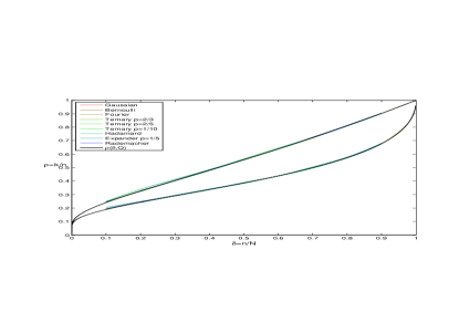
Figure 4. Upper curves: level curves of 50% success rate for each non-Gaussian suite in Table 1 with nonnegative coefficients, as well as for the Gaussian suite. Asymptotic phase transition $\rho(\delta;T)$ overlaid in black. Lower curves: level curves for 50% success rate for each suite in Table 1 with coefficients of either sign, and for Gaussian suite. Asymptotic phase transition $\rho(\delta;C)$ overlaid in black.

At first glance, figure 4 shows excellent agreement between the actual empirical results in each matrix ensemble and the asymptotic theory for the Gaussian. This is not very surprising for $A$ from the Gaussian ensemble; it merely proves that the large-$N$ polytope theory works accurately already at moderate $N=1600$. For the other ensembles there is not, to our knowledge, any existing theory suggesting what we see so clearly here: phase transition behaviour in non-Gaussian ensembles that accurately matches the Gaussian case (compare §4).

3.2. Universality hypothesis

Figure 4 suggests to us the following

Hypothesis. Universality of Phase Transitions. Suppose that the $n$ by $N$ matrix $A$ is sampled randomly from a “well-behaved” probability distribution. Suppose that the $N$ by $1$ vector $x_{0}$ is sampled randomly from the set of $k$-sparse vectors, either with or without positivity constraints on the nonzeros of $x_{0}$. The observed behaviour of solutions to $(LP)$ and $(P_{1})$ will exhibit, as a function of $(N,n,k)$, success probabilities matching those which are proven to hold when sampling from the Gaussian distribution with large $N$.

This hypothesis really contains two assertions: (a) that many matrix ensembles behave like the Gaussian; and (b) that moderate-sized $N$ exhibit behaviour in line with the $N\rightarrow\infty$ asymptotic.

The hypothesis also contains an element of vagueness, since we do not know at the time of writing how to delineate the ensembles of random matrices over which Gaussian-like behaviour will hold. Of course universality results are well known in probability theory; the Central Limit Theorem is the most well-known universality result for the distribution of sums of independent random variables. The precise universality class of the Gaussian distribution for such sums was only discovered two centuries after the phenomenon itself was identified. Apparently we are here at the stage of just identifying a comparable phenomenon. We hope it does not take two centuries to identify the corresponding universality class!

Clarification 1. In fact, our hypothesis could also be called a rigidity of the phase transition – it is invariantly located at the same place in the phase diagram across a range of matrix ensembles. In statistical physics, universality of a phase transition means something different, and much weaker – not a rigidity, but instead a flexibility of the location of a phase transition while preserving an underlying structural similarity. Our hypothesis is far stronger.

Clarification 2. In fact, there are trivial counterexamples to the hypothesis; for example the matrix $A$ of all ones does not generate any useful phase transition behaviour.

3.3. Experimental procedure

We conducted a Monte Carlo experiment to test the Universality Hypothesis.

The general procedure was like our earlier exploratory studies. We call a suite a distribution of problem instances $(y,A)$ fully specified by two factors: (1) the ensemble of matrices $A$ and (2) the ensemble of coefficients $x_{0}$ generating $y=Ax_{0}$. Matrix ensembles include Bernoulli, Ternary, … Coefficient ensembles studied here have vectors of $N$ coefficients with only $k$ nonzeros, in sites chosen at random. The positive sign coefficient ensemble indicated by $+$ has all nonzeros drawn uniformly from $[0,1]$. The signed coefficient ensemble indicated by $\pm$ has nonzeros drawn uniformly from $[-1,1]$. For each suite we visited a collection of triples $(N,n,k)$. At each triple we drew a sequence of random problem instances of the given size and shape from the given problem suite. We then ran optimization software to compute the solution of the random problem. We computed observables from the obtained solution, in particular the binary observable ExactRecon, which takes the value 1 when the obtained solution is equal to the true solution within 6 digits accuracy, and zero otherwise.

We aimed to be confirmatory rather than exploratory: to use formal inferential tools, and carefully explain apparent departures from our hypothesis. Our experiments differed from earlier efforts in scope and attention to detail.

• Scale. We performed 2,948,000 separate optimizations spanning 16984 different situations. Our computations required the use of as many as 200 CPUs in an available cluster and overall required 6.8 CPU years. We considered 16 problem suites based on 8 different matrix ensembles; see table 1. The scope of previous exploratory studies, which can be measured in CPU-days, is tiny by comparison.

• Calibration. The vast majority of our experimental computations relied on Mosek, a commercial package. We made runs comparing the results with CVX, a popular open-source optimization package. We believe our results are consistent across optimizers.

3.4. Inferential formulation

Rather than go on a fishing expedition, from the outset we chose to frame our evaluation of the evidence using standard inferential procedures.

• Two-sample comparisons. The strict form of the Universality Hypothesis says that the probability of unique solution under the Gaussian Ensemble is the same as the probability of unique solution at each other ensemble in the universality class. It follows that we may compare two sets of results at the same problem size, one with the Gaussian ensemble and one where everything else in the problem is the same except that a specific non-Gaussian ensemble is used. If at each ensemble we generate $M$ problem instances and obtain $M$ realizations of the observable ExactRecon, strict universality requires that the number of successes in each ensemble have a binomial probability distribution with the same success probability in both ensembles. Hence, the hypothesis really amounts to the assertion that two binomial distributions are the same. We proceed with traditional tests for equality of two binomial distributions. We chose to work with the $Z$-score:

  (3.5) $$Z(\hat{p}_{0},\hat{p}_{1};M)=\frac{\hat{p}_{0}-\hat{p}_{1}}{\hat{SD}(\hat{p}_{0}-\hat{p}_{1};M_{0},M_{1})}.$$

  Here $\hat{p}_{i}$ denotes “the fraction of cases where Exact Recon = 1 in ensemble $i$”, and $\hat{SD}(\hat{p}_{0}-\hat{p}_{1};M_{0},M_{1})$ is the appropriate standard error for comparing proportions with possibly unequal sample sizes $M_{i}$. In this comparison $\hat{p}_{0}$ describes the Gaussian baseline experiment, and $\hat{p}_{1}$ describes the non-Gaussian alternative experiment. Under the Universality Hypothesis, $Z$ has an approximate standard normal distribution.

  Reducing our problem merely to consideration of $Z$-scores we can formalize our hypothesis:

  Strong Null Hypothesis: The $Z$ scores have an approximate $N(0,1)$ distribution at each value of $(k,n,N)$.

• Study of asymptotics with problem size. The Strong Null Hypothesis seems implausible a priori on the strength of experience from other settings.

  Consider another setting where the Gaussian distribution is universal: the central limit theorem. There, although the Gaussian distribution provides the correct limiting behaviour, there are well-understood departures from Gaussian behaviour at small problem sizes. Such departures of course decay with increasing problem size. The theory of Edgeworth expansions shows that such deviations from Gaussianity decay with problem size according to a specific power of size. Hence, for a symmetric distribution, we will see deviations of order $1/(\mbox{problem size})$ and, for an asymmetric one, deviations of order $1/\sqrt{\mbox{problem size}}$ occur.

  Analogously, in this setting we may see systematic behaviour of the $Z$-scores varying with problem size $N$ and perhaps also with $k$. We used three problem sizes - $N=200,400$ and $1600$ - so we might identify trends in the $Z$-scores with problem size.

  Weak Null Hypothesis: The $Z$-scores exhibit discrepancies from the standard $N(0,1)$ distribution (e.g. in means, variances, tail probabilities) which decay to zero with increasing $N$.

3.5. Results

Results of our experiment were already summarized in figure 4. For each suite in table 1, for each value of $\delta=n/N$, we measured the value of $\rho=k/n$ at which the empirical probability of success crossed 50%. Each of the 18 different curves in figure 4 presents results for one suite; each one depicts the 50% success rate curves as a function of $\delta$. These “empirical $\rho$ curves” exhibit very strong visual agreement with the corresponding theoretical curves $\rho(\delta;T)$ and $\rho(\delta;C)$.

3.5.1. Raw $Z$-scores

Formal statistical tests are much more sensitive and objective than visual impressions. Figure 5 displays the $Z$-scores (3.5) for two-sample comparisons between the Gaussian ensemble with nonnegative coefficients and the odd numbered suites; similarly, figure 6 presents two-sample comparisons between the Gaussian ensemble and the odd numbered suites. The eight panels in each figure depict differences between each of the non-Gaussian ensembles and the Gaussian ensemble. The problem shape $\delta=n/N$ runs along the horizontal axis; these plots display results for $N=200,400,1600$ all combined.

The vast majority of the $Z$-scores in these displays fall in the range $-2,2$.

Finding 1: The $Z$-scores in bulk are consistent with our hypothesis of no difference between the distributions.

In effect, our experiment conducted 16,984 hypothesis tests and found relatively few ‘significant differences’ at the individual test level.

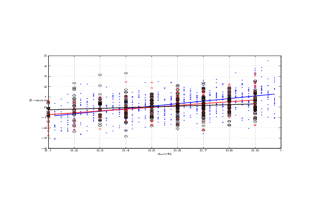
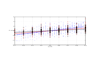
(a) Bernoulli	(b) Fourier
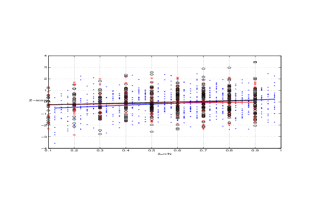
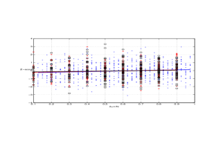
(c) Ternary (1/3)	(d) Ternary (2/5)
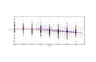
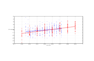
(e) Ternary (1/10)	(f) Hadamard
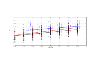
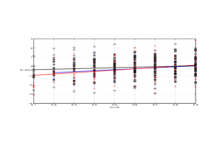
(g) Expander	(h) Rademacher

Figure 5. Raw $Z$-scores comparing success rate of reconstruction by (LP) for $A$ from the Gaussian ensemble vs. success rate for $A$ from suites 3,5,7,9,11,13,15, and 19 in Table 1. Panels (a-e,g-h): suites 3,5,7,9,11,15, and 19, respectively. Blue dots: $N=200$; red crosses: $N=400$; black circles: $N=1600$. Linear fits to the raw $z$-scores in matching colors. Panel (f): Hadamard case, dyadic $N$ only. Blue dots: $N=256$; red crosses: $N=512$.

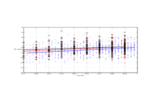
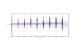
(a) Bernoulli	(b) Fourier
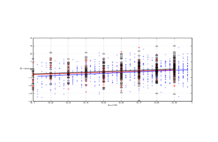
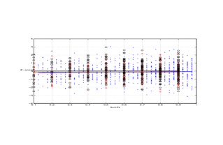
(c) Ternary (1/3)	(d) Ternary (2/5)
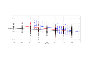
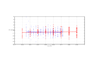
(e) Ternary (1/10)	(f) Hadamard
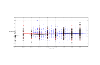
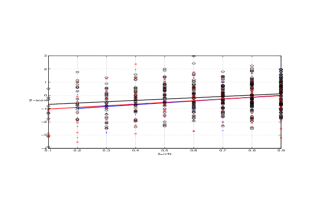
(g) Expander	(h) Rademacher

Figure 6. Raw $Z$-scores comparing success rate in reconstruction by (P1) for $A$ from the Gaussian ensemble vs. success rate for $A$ from suites 4,6,8,10,12,14,16, and 20 in Table 1. Panels (a-e,g-h): suites 4,6,8,10,12,16, and 20 respectively. Blue dots: $N=200$; red crosses: $N=400$; black circles: $N=1600$. Linear fits to the raw $z$-scores in matching colors. Panel (f): Hadamard case, dyadic $N$ only. Blue dots: $N=256$; red crosses: $N=512$.

3.5.2. Rejection of strict universality

There are marked ‘tilts’ in the display of $Z$-scores in figures 5 and 6; linear trends with $\delta$ are visually evident. Consider the general mean-shift model

$$Z(\delta,\rho;N,E)=\mu(\delta;N,E)+{\mathcal{Z}},$$

where ${\mathcal{Z}}\sim N(0,1)$ is standard normal. This expresses the idea that the observed $Z$-scores exhibit ‘drift’ as a function of $\delta$ and $N$, but otherwise have the expected statistical properties of such scores.

If $\mu$ is not truly zero in this model, then of course the null hypothesis of no difference fails. In our setting this means that the Gaussian ensemble does not give truly the same success probabilities as the ensemble being compared to it. Our analysis below rejects the hypothesis that $\mu=0$:

Finding 2: The $Z$-scores are not consistent with the hypothesis of Strict Universality. Exact finite-problem-size agreement of success probabilities $p_{1}$ and $p_{0}$ between each alternative ensemble and the Gaussian ensemble is not supported by our experiments.

3.5.3. Non-rejection of weak universality

We reformulate the weak universality hypothesis in terms of moments:

Refined Null Hypothesis: for each ensemble $E$, $\mu(\delta;N,E)$ tends to zero with increasing $N$, and the standard deviation of $Z$ scores approaches $1$.

This hypothesis has a clear motivation. Earlier displays aided the eye with lines fitted to the means. Evidently, the mean $Z$-scores within a given suite are generally closer to zero for $N$ large than for $N$ small. Hence, in an informal appraisal, the refined null hypothesis seems quite plausible. Inspired by the ‘Higher Criticism’ (see Donoho & Jin (2009)), we compare the observed bulk distribution of $Z$ scores with the theoretical distribution $N(0,1)$. Table 2 shows roughly as many large $Z$ scores as one would expect under the null hypothesis.

$N$	#$\{i:|Z_{i}|<1\}$	#$\{i:|Z_{i}|<2\}$	#$\{i:|Z_{i}|<3\}$	$M$
200	101 / 99.67	142 / 139.4	148 / 145.6	148
400	146 / 140.6	199 / 196.6	208 / 205.4	208
1600	258 / 267.6	380 / 374.2	394 / 390.9	394

Table 2. Higher Criticism style analysis of residual $Z$-scores in suite 19. Cell contents: observed counts/expected counts.

Finding 3: The $Z$-scores do not reject the hypothesis of Weak Universality. The difference between success probabilities $p_{1}$ and $p_{0}$ for each alternative ensemble and the Gaussian ensemble can be adequately modelled as a matrix-dependent random variable with stochastic order $p_{1}(A)-p_{0}(A^{\prime})=O_{p}(N^{-1/2})$, where $A$ and $A^{\prime}$ are realizations in the two matrix ensembles.

3.6. Results not presented in the main text

In the appendix, we present a fuller record of our analyses. Key points include the following.

• Transition zone scaling with $N$. We verified that the width $w(\delta,N;Q)$ of the zone where success probability drops from 1 to 0 scales as $w\propto N^{-1/2}$.

• Adequacy of probit model. We verified that the success rate varies with $\rho$ as a Probit function $\overline{\Phi}((\rho-\rho(\delta;Q))/w(\delta,N;Q))$. Here $\overline{\Phi}$ is the Gaussian survival function and $w$ is the transition width.

• Exceptional Ensembles. It is evident from figures 5-6 that, at small $N=200$, certain ensembles offer a relatively poor match to the Gaussian case. Most of these discrepancies can be accounted for by saying that in these exceptional ensembles, at small problem sizes, the level curve for 50% success rate is shifted noticeably below the 50% curve for the Gaussian ensemble. However, at the larger problem size $N=1600$, both the shift and the exceptional character of the ensembles are no longer evident. For details, see the appendix.

3.7. Limitations of our conclusions

We considered a limited set of matrix ensembles in this study. The ensembles are not all based on iid elements – there are dependencies among rows in the Fourier and Hadamard ensembles and among columns in the Expander ensemble. Even so, there is a certain air of ‘orthogonality’ or ‘weak independence’ in these examples.

There are exceptions to the pattern presented here. The classical example of cyclic polytopes shows that (LP) can have a notably higher success rate for very special matrices than it does for random matrices (Donoho & Tanner, 2005$a$).

In addition to forward stepwise regression, (LP) and (P1), there are several competing algorithms which we do not study here. Maleki & Donoho (2009) conducted extensive empirical testing of many such algorithms and observed clear phase-transition-like behaviour, which varies from algorithm to algorithm and from the results presented here. Unlike the phase transitions presented here, which match theoretical results in combinatorial geometry, the phase transitions observed for competing algorithms are not yet supported by theoretical derivations.

4. Conclusion, and a glimpse beyond

Certain phase transitions in high-dimensional combinatorial geometry have been derived assuming a Gaussian distribution. We had informally observed that the Gaussian theory seemed approximately right even in some non-Gaussian cases. In this study, we made extensive computational experiments with more than a dozen matrix ensembles considering millions of instances at a range of problem sizes. Empirical results for both Gaussian and non-Gaussian ensembles show finite-$N$ transition bands centred around the asymptotic phase transition derived from a Gaussian assumption. The bands have a width of size $O(N^{-1/2}$), consistent with the proven behaviour for the Gaussian ensemble (Donoho & Tanner 2008$b$). Such behaviour at non-Gaussian ensembles goes far beyond current theory. Adamczak et al. (2009) proved that, for a range of random matrix ensembles with independent columns, there is a region in the phase diagram where the expected success fraction tends to one, but there is no suggestion that this region matches the region for the Gaussian.

We used standard two-sample statistical inference tools to compare results from non-Gaussian ensembles with their Gaussian counterparts at the same problem size and sparsity level. We observed fairly good agreement of the two-sample $Z$-scores with the null hypothesis of no difference; however, fitting a linear model to an array of such $Z$-scores we were able to identify statistically significant trends of the $Z$-scores with problem size and with undersampling fraction $\delta=n/N$. The fitted trends vary from ensemble to ensemble, decay with problem size, and are consistent with weak, ‘asymptotic’, universality but not with strong, finite-$N$, universality.

Our evidence points to a new form of ‘high-dimensional limit theorem’. There is some as-yet-unknown class of matrix ensembles that yield phase transitions at the same location as the Gaussian polytope transitions. Delineating this universality class seems an important new task for future work in stochastic geometry.

5. Appendix: suplementary statistical analysis

We present details of the data analysis.

Gaussian ensemble. We study the basic properties of success probabilites at the Gaussian ensemble, as a function of $\delta$ and $\rho$.

• Transition zone scaling with $N$. We quantify the width $w(\delta,N;Q)$ of the zone where success probability drops from 1 to 0. We verify that our measurement scales as $N^{-1/2}$.

• Adequacy of Probit/Logit models. We verify that the success probability varies with $\rho$ approximately as a Probit function $\overline{\Phi}((\rho-\rho(\delta;Q))/w(\delta,N;Q))$. Here $\overline{\Phi}$ is the Gaussian survival function and $w$ is the transition width. A logit function fits just about as well.

Analysis of $Z$-scores. We compare success probabilities at the non-Gaussian ensembles to those at the Gaussian using $Z$-scores arising from two-sample tests for binomial proportions.

• Methodology of $Z$-score comparison. We verify that in the null case of no difference, our methodology indeed finds no difference; we also verify that in the case of known difference, it indeed finds a difference.

• Scaling of moments with $N$. We identify nonzero means in the $Z$-scores, and show that the scaling law $\mu(\delta,N;E)=O(1/N^{1/2})$ best describes the data.

• Exceptional ensembles. Two matrix ensembles exhibit substantial lack-of agreement with the others (e.g. some individual $Z$-scores as large as 20) for $n$ small. In effect the location for 50% success in those ensembles obeys a slight shift away from $\rho(\delta;Q)$, of order $w$. While this is an asymptotically negligible shift, failing to model it causes a noticeable lack of fit at $N=200$ and $n$ small. This lack of agreement is observed to dissipate as $n$ increases.

• Validation ensembles. Two matrix ensembles were studied only after all other analysis had been completed. Using the models arrived at in the prior analysis without changing the model form, we found that the same models describe the validation ensembles adequately, reinforcing the validity of our analysis.

All noticeable elements of lack of fit are best accounted for as evidence of effects consistent with the weak universality hypothesis.

5.1. Experiments conducted

5.1.1. Framework

Terminology:

• We study $n\times N$ random matrices $A$, $N>n$.

• A matrix ensemble is a generating device for $n\times N$ matrices. We report here results on the 9 different random matrix ensembles , listed in table 1.

• We generate vectors $y=Ax_{0}$ where $x_{0}$ has $k$ nonzeros.

• The nonzeros in $x_{0}$ are either drawn uniformly from $(0,1)$ or $(-1,1)$, designated as coefficients $+$ and $\pm$ respectively.

• The instances $(y,A)$ where the underlying $x_{0}$ is nonnegative by intent are then processed using an optimizer to approximately solve $(LP)$. The instances where the underlying $x_{0}$ can be of both signs are processed by using an optimizer to approximately solve $(P_{1})$.

• The optimizer is presented with the problem instance $(y,A)$, but not $x_{0}$.

• After running the optimizer, we measure ExactRecon, which takes the value 1 when the obtained solution $x_{1}$, say, is equal to the desired solution $x_{0}$, within 6 digits accuracy. It is zero otherwise.

• We conduct $M$ independent replications at each fixed combination of $N,n,k$, matrix ensemble, and coefficient type.

• The variable $S$ totals the number of times ExactRecon was $1$ in the $M$ replications. Results are tabulated in a data file with column headings

  E N n k M S
  

  Here $E$ is an integer code specifying the suite of problem instances. Such a suite specifies both the matrix ensemble (eg Gaussian, Bernoulli, Rademacher, …) and the coefficient type ($+$ or $\pm$). For each matrix ensemble we consider both coefficient types.

• For analysis and presentation, we use coordinates $\delta=n/N$, the matrix ‘shape’, and the solution sparsity level $\rho=k/n$. We generally consider the success fraction $\hat{p}=S/M$.

• The most important structure of the dataset concerns the constant-$\delta$ slices, where $n$, $N$, $E$ are held constant and $k$ is varying. The success fraction $\hat{p}(k,n,N;E)$ is generally monotone decreasing in such a slice: monotone decreasing in $k$ for fixed $n$, $N$, and $E$.

• We focus on what is called the $LD50$ in bioassays, the 50% quantal response more generally. It is the value of $k/n$ where $S/M$ is expected to be $1/2$, for fixed $n$,$N$, $E$.

5.1.2. Range of experiments

For each suite in table 1 and each combination of $N,n,k$, we consider $M=200$ different problem instances $(y,A)$ each one drawn randomly as above. Each suite is compared with a “baseline” of either suite 1 or 2 for the same combination of $N,n,k$ but a larger independent draw of $M=1000$ problem instances. We varied the matrix shape $\delta=n/N$, and the solution sparsity levels $\rho=k/n$. At problem size $N=1600$, we varied $n$ systematically through a grid ranging from $n=160$ up to $n=1440$ in 9 equal steps. The ‘signal processing language’ event ‘exact reconstruction’ corresponds to the ‘polytope language’ event ‘specific $k$-face of $Q$ is also a $k$-face of $AQ$’. In both cases we speak of success, and we call the frequency of success in $M$ empirical trials at a given $(k,n,N)$ the success rate. At each combination $N,n$, we varied $k$ systematically to sample the success rate transition region from $5\%$ to $95\%$.

5.1.3. Suites studied

In sections 3-7 we report details about experiments with the non-Gaussian suites $3-12$ and $15-16$ listed in table 1. As it happens, after the analysis of these suites was conducted, data became available for four other suites, based on the Hadamard and Rademacher ensembles. The analysis of those suites will be reported only in section 8. The Rademacher ensemble, suites 19 and 20, generated data with the same problem sizes and other parameters as suites $3-12$ and $15-16$. Our study of the Hadamard ensemble, suites 13 and 14, is restricted since only two problem sizes $N=256$ and $N=512$ were run.

5.2. Behaviour of the Gaussian ensemble

In this section, we restrict attention to the Gaussian ensemble, suites 1 and 2, and investigate these questions:

• Width of transition zone. How does the width $w(\delta;N,Q)$ of the transition zone at phase transition vary, as a function of $N$?

• Quantal Response Profile. How does the probability of success vary as a function of the reduced $(\rho-\rho(\delta;Q))/w(\delta;N,Q)$? Where $\rho=k/n$ and $\delta=n/N$.

• Behaviour of $LD50$. In what manner does the empirical 50% point of the quantal response function approach the underlying asymptotic limit $\rho(\delta;Q)$?

The Gaussian ensemble is an appropriate place to focus attention, because:

• A complete, rigorous understanding of the asymptotic behaviour exists in the Gaussian case (Donoho & Tanner 2009$a$); we know that as $N\rightarrow\infty$ with $\delta$ fixed and $\rho$ fixed away from $\rho(\delta,Q)$, the success probability tends to either zero or 1. So we know that there is a transition zone, and that its width tends to $0$ as $N\rightarrow\infty$.

• A rigorous set of finite-$N$ bounds has been rigorously proven (Donoho & Tanner 2008$b$); we know that the width scales like $O(1/\sqrt{n})$.

Hence, there are rigorous theoretical constraints: we know the phase transition exists asymptotically and we can constrain its width.

5.2.1. Modelling the quantal response function

In the field of bioassays, the Quantal response function gives the probabiliy of organism failure (eg death) as a function of dose. In our setting, the analogous concept is the probability of algorithm failure at a fixed problem size $n,N$ as a function of $\rho=k/n$, the “complexity dose”.

Considering a constant-$\delta$ slice at the Gaussian ensemble, suite 2, we see a roughly monotone increasing probability of failure as a function of $k/n$. Figure 7 presents the fraction of success $S/M$ as a function of $k/n$, at three incompleteness ratios $\delta=n/N$.

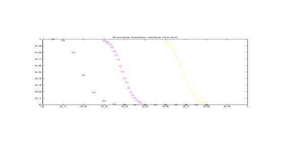
Figure 7. Empirical success fraction at Gaussian ensemble, suite 2, for $\delta=.1$ (black circles), $\delta=.5$ (magenta triangles), $\delta=.9$ (yellow diamonds). Horizontal axis: $\rho=k/n$; vertical axis: success fraction $S/M$. Data result from $M=1000$ trials at $N=1600$.

A Probit model for the dose response states that, for parameters $a$, and $b$, the expected fractional success rate is given by

(5.6) $${\mathcal{E}}(S/M)=\bar{\Phi}(a(\delta)+b(\delta)\rho)$$

where $\bar{\Phi}$ is the complementary normal distribution, and ${\mathcal{E}}$ denotes expectation. Figure 8 presents a first pass at checking the suitability of such a model. It identifies empirical estimates of the points where ${\mathcal{E}}(S/M)=\alpha$ for $\alpha\in\{1/4,1/2,3/4\}$. and then chooses $a$ and $b$ in relation (5.6) to match those. It displays the raw data, the model curves, and residuals from the model.

Figure 8. Crude probit modeling of dose response. Rows for $\delta=.1$, $\delta=.5$, $\delta=.9$. First column: same as in figure 7 for suite 2, $N=1600$ and $M=1000$. Second Column: data and probit model. Third Column; Residuals.

It is standard in biostatistics to fit generalized linear models to such data; the binomial response model is appropriate here. Such models take the form

$$S\sim Bin(p(\delta,\rho),M)$$

where the success probability $p(\delta)$, after a fixed transformation $\eta()$ , obeys a linear model:

$$\eta(p(\delta,\rho))=a(\delta)+b(\delta)\rho;$$

the function $\eta$ is called the link function.

We considered three standard link functions: the logit, probit and cauchyit links. Figure 9 presents fitted models and what the statistics analysis package R calls the working residuals for these three links. In fact the best loglikelihood is achieved among the three at the probit link, but there is a large residual at the most extreme response; it seems the probit link goes to zero too fast (this is not unexpected, owing to the ’thin tails’ of the normal distribution, and also owing to the finite-N large deviations analysis in Donoho and Tanner (2008$b$)). The logistic link is nearly as good in deviance or likelihood senses, makes sense on theoretical grounds and gives more balanced residuals. (Note however, that as figure 8 showed, the Probit fit is adequate as long as we look at ordinary rather than the more statistically sensitive working residuals.)

Figure 9. GLM modeling of dose response for suite 2 ($N=1600$ and $M=1000$) with three links; case $\delta=.1$. First Column: fit with Logit link. Second Column: fit with Probit link. Third Column: fit with Cauchyit Link. First Row: Fits. Second Row: Working Residuals.

We used R to fit these models; this has the advantage of automatically providing standard inferential tools – confidence bounds for $a$ and $b$ and goodness-of-link tests.

5.2.2. Behaviour of $LD50$

In bioassays, the $LD50$ is the dose that corresponds to 50/50 chance of failure. This can be estimated from binomial response data in two ways.

The first, ‘nonparametric’ method finds the largest ratio $k/n$ where $S>M/2$ for a given $n$, $N$ and $E$. We found a slight refinement useful: we fit a linear spline to the success ratios and solved for the (smallest) value of $\delta$ where the spline crosses $50$%.

Using this method, we obtained table 3, which presents, for suite 2 and $M=1000$, the difference between the estimated $LD50$ and the theoretical large $N$ limit.

$\delta$	200	400	1600
0.2	0.0114	0.00410	0.001799
0.3	0.0079	0.00476	0.001179
0.4	0.0043	0.00444	0.001037
0.6	0.0053	0.00198	0.000760
0.7	0.0048	0.00380	0.001649
0.8	0.0082	0.00280	0.001171

Table 3. Difference between empirically estimated $LD50$ of suite 2 with $M=1000$ samples and the corresponding asymptotic limit $\rho(\delta;C)$

Evidently, the $LD50$ is approaching the expected phase transition with increasing $N$. To quantify this effect, we have table 4, which shows that the $LD50$ typically approaches its limit at roughly the rate $1/N$.

Quantity	200	400	1600
median $N^{1/2}(LD50-\rho(\delta))$	0.094	0.079	0.047
median $N(LD50-\rho(\delta))$	1.324	1.581	1.881

Table 4. Median across $\delta$ of the scaled difference between empirically estimated $LD50$ of suite 2 with $M=1000$ and the corresponding asymptotic limit $\rho(\delta;C)$

5.2.3. Transition zone width

We can define the $\alpha$-width of the transition zone as the horizontal distance between $p=\alpha$ and $p=1-\alpha$ on the dose-response.

We again can measure this nonparametrically and parametrically. We present here a nonparametric analog based on fitting splines to the empirical success fractions and measuring the $\alpha=0.1$ and $1-\alpha=0.9$ quantile locations. We then normalize by the corresponding distance on the standard Probit curve

$$w=w_{0.1}=\frac{q_{0.9}-q_{0.1}}{\Phi^{-1}(0.9)-\Phi^{-1}(0.1)}.$$

Table 5 presents values of $\sqrt{N}\cdot w(\delta,N)$ for suite 2 with $M=1000$.

$\delta$	$N=200$	$N=400$	$N=1600$
0.2	0.7277	0.6691	0.6367
0.3	0.6567	0.6535	0.6780
0.4	0.6530	0.6464	0.6240
0.6	0.6328	0.6663	0.6420
0.7	0.6413	0.6690	0.6384
0.8	0.6708	0.6841	0.6809

Table 5. Scaled values $\sqrt{N}w(\delta;N)$ for suite 2 with $M=1000$.

5.3. Methodology of $Z$-score comparison

How does the methodology of $Z$-score comparison work on cases where we know the ground truth – both where we know there is no difference and we know there is an asymptotic difference? For each of the suites in table 1 the suite with $M=200$ is compared against suite 1 or 2 with $M=1000$ independent problem instances for the same values of $N,n,k$. Suites 1 and 2 with $M=1000$ form the baseline against which all $Z$-scores are calculated. Unless specified otherwise, suites with the same coefficient sign are compared; for example suite 9 is compared with suite 1 and suite 16 is compared with suite 2.

5.3.1. Under a true null hypothesis

When the two problem settings being compared are simply replications of the same underlying conditions, we can be sure that $H_{0}$: no difference is true. We compare here suites 1 and 2 with $M=200$ against the baseline experiments of suites 1 and 2 with $M=1000$. This follows the same procedure as will be conducted later when comparing non-Gaussian ensembles against the baseline.

Figure 10 Panel(a) presents the bulk distribution of $Z$-scores for suite 2; Panel (b) presents the bulk distribution of $Z$-scores for suite 1. The figure presents PP-plots: the fraction of $Z$-scores exceeding a threshold versus the fraction to be expected at the standard Normal. If the $Z$-scores were exactly standard normal, these plots would be close to the identity line, which is, in fact what we see.

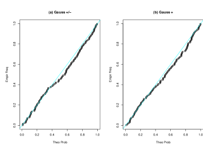
(a)                              (b)

Figure 10. PP Plots of $Z$-scores comparing success frequencies under one set of realizations from the Gaussian matrix ensemble ($M=200$) with an independent realization of success frequencies from the Gaussian ensemble ($M=1000$). Panel (a): suite 2. Panel (b): suite 1.

In quantitative terms, we have table 6.

Suite 1: Gaussian ensemble, positive coefficients
$N$	#$\{i:|Z_{i}|<1\}$	#$\{i:|Z_{i}|<2\}$	#$\{i:|Z_{i}|<3\}$	$\#$
200	29/54	49/54	54/54	54
400	40/63	60/63	63/63	63
1600	45/63.6	61/63	63/63	63
Suite 2: Gaussian ensemble, coefficients of either sign
200	41/55	53/55	55/55	55
400	38/63	60/63	63/63	63
1600	42/63	62/63	63/63	63

Table 6. Occurrences of $Z$-scores under the true null hypothesis. Suites 1 and 2 self comparison of $S/M$ with $M=200$ against the basline suites 1 and 2 with $M=1000$. Cell contents: Observed Counts/Total Counts.

Table 6 shows that of 180 $Z$-scores associated with comparisons of suite $1$, 170 were less than $2$ in absolute value; for $94.4$ % – very much in line with an assumed standard $N(0,1)$ null distribution. It also shows that of 181 $Z$-scores associated with comparisons of suite $2$, 175 were less then $2$ in absolute value; for $96.7$ % – very much in line with an assumed standard $N(0,1)$ null distribution. We thus see that under a true null hypothesis, our $Z$-scores behave largely as if they were $N(0,1)$. This is an observation that needed to be checked, since $Z$-scores, when constructed in the way we have done so here, only are known to have an asymptotically normal distribution.

Figures 5 and 6 presented $Z$-scores in scatterplots of $Z(k,n,N;E)$ versus $\delta$ comparing non-Gaussian ensembles with Gaussian ensembles; what happens when we have a true null hypothesis?

Figure 11 (a) and (b) presents the $Z$-scores for suites 1 and 2 respectively with fitted lines modelling the dependence on $\delta$. In principle, the $Z$-scores all have mean zero and there is no expected trend. However, owing to sampling fluctuation, we obtain nonzero intercepts and slopes. Table 7 shows the results that obtained in this truly null case. We learn from this that fitted intercepts and slopes of about the size indicated in the table can be viewed as consistent with a true null hypothesis.

Suite 1                                  Suite 2

$N$	$a$	$b$
200	0.127	-0.242
400	-0.103	0.451
1600	0.133	-0.002

$N$	$a$	$b$
200	0.002	0.102
400	0.109	0.445
1600	-0.166	0.166

Table 7. Linear fits to $Z$-scores $Z\sim a+b\delta$ under the true null hypothesis. Suites 1 and 2. $a$ intercept; $b$ slope

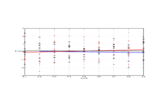
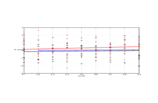
(a)	(b)

Figure 11. $Z$-scores under true null hypothesis, and linear fit. Panel (a): suite 1. Panel (b): suite 2.

5.3.2. Under a true alternative hypothesis

Is our methodology powerful? Can it detect any differences from null?

To study this question, we considered a simple and blatant mismatch: compare suite 1 with $M=200$ against the suite 2 with the baseline $M=1000$.

The baseline, suite 2, should reflect a transition near $\rho(\delta;C)$ while the comparison group, suite 1, should reflect a transition near $\rho(\delta;T)$. As these two curves are very different we should see this reflected in the $Z$-scores. And we do. Figure 12 shows the QQ-plot, which is noticeably far from the identity line.

Figure 12. QQ plot of $Z$-scores comparing success frequencies of suite 1 ($M=200$) to an independent realization of success frequencies from suite 2 ($M=1000$). In this plot, the $M=200$-based frequencies describe success in solving $(LP)$ when the nonzeros in $x_{0}$ are positive, the $M=1000$-based frequencies describe success in solving $(P_{1})$ when the nonzeros in $x_{0}$ are of either sign. The two ensembles are proven to have different phase transitions. The values on the $Y$ axis are far away from $0$.

5.4. Bulk behaviour of $Z$-scores

In figures 13-15 we present a sequence of QQ plots showing the bulk distribution of $Z$-scores for suites $3-12,15-16$ at $N=200$, $400$ and $1600$. In each plot the identity line is also displayed; if the $Z$-scores had truly a standard normal distribution, they would oscillate around this line.

While in most suites we see a good match between the $Z$-scores and the standard normal already at $N=200$, it is not until $N=1600$ when every ensemble seems to yield approximately $N(0,1)$ scores. Even then, suites 11 and 12 (Ternary (1/10)) exhibit some noticeable deviations. These effects are apparent for small $n$. In fact, at small $n$, trivial linear dependencies are found among the columns of typical random $A$ at these ensembles. Such linear dependencies force affine dependencies which force lost polytope faces. Consequently, the observed $S/M$ will be decreased, this effect is discussed further in §5.7.

This is consistent with our conclusions in the main text that strict finite-$N$ universality does not hold, but a weaker notion of asymptotic universality does hold.

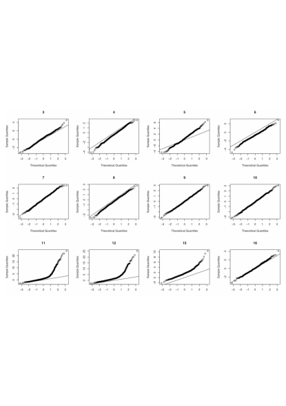
Figure 13. $Z$-scores at $N=200$ for suites 3-12,15-16.

Figure 14. $Z$-scores at $N=400$ for suites 3-12,15-16.

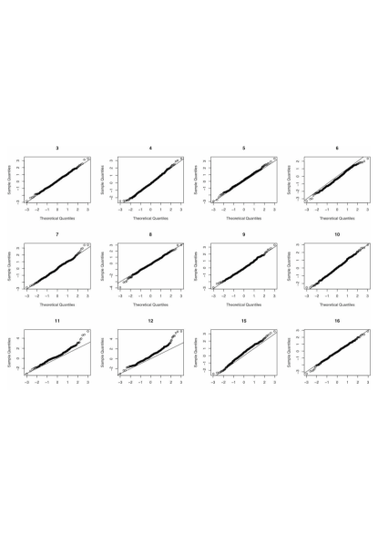
Figure 15. $Z$-scores at $N=1600$ for suites 3-12,15-16.

5.5. Linear modeling of the $Z$-scores

The QQ Plots of $Z$-scores in figures 13-15 show that suites 11, 12, 15, and 16 (the highly sparse matrix suites) behave somewhat differently than other suites.

We now report results excluding those suites, and focus instead on suites 3-10. The excluded suites $11-12,15-16$ will be discussed in §5.7.

In the main text we reported fits explaining the observed $Z$-scores using two models of the form,

(5.7) $$\mu(\delta;N,E)=\alpha(N,E)+\beta(N,E)(\delta-1/2),$$

where

(5.8) $$\alpha(N,E)=\alpha_{0}(E)+\alpha_{1}(E)/N^{1/2},\qquad\beta(N,E)=\beta_{0}(E)+\beta_{1}(E)/N^{1/2}.$$

We considered two such models, one with the restrictions $\alpha_{0}=0$ and $\beta_{0}=0$, and one without.

We first report results using the submodel $\alpha_{0}=0$ and $\beta_{0}=0$, and later the full model, without the restriction. The display below shows the output of the $R$ linear model command for the restricted model. The symbol de denotes $\delta-1/2$ and the symbol probSize denotes $1/\sqrt{N}$. The output lists interaction terms such probSize:En. It turns out that $\alpha_{1}(N,E)$ is the sum of probSize and probSize:En. Similarly $\beta_{1}(N,E)$ is the sum of probSize:de and probSize:En:de.

lm(formula = Z ~ probSize * E * de - E * de - E - de - 1, subset = subE)

Residuals:
      Min        1Q    Median        3Q       Max
-3.966108 -0.703283 -0.003336  0.691872  4.309933

Coefficients: (1 not defined because of singularities)
                        Estimate    Std. Error t value Pr(>|t|)
probSize         -1.7714     0.5752  -3.080  0.00208 **
probSize:E3       2.5960     0.7955   3.263  0.00111 **
probSize:E4      -6.1540     0.8141  -7.560 4.40e-14 ***
probSize:E5       3.3350     0.7972   4.183 2.90e-05 ***
probSize:E6      -9.0306     0.8128 -11.110  < 2e-16 ***
probSize:E7      -0.6122     0.7957  -0.769  0.44168
probSize:E8      -4.8878     0.8117  -6.022 1.79e-09 ***
probSize:E9       0.4795     0.7964   0.602  0.54715
probSize:E10          NA         NA      NA       NA
probSize:de      32.4608     2.2249  14.590  < 2e-16 ***
probSize:E4:de  -13.3427     3.0552  -4.367 1.27e-05 ***
probSize:E5:de   38.3394     3.1584  12.139  < 2e-16 ***
probSize:E6:de  -25.7357     3.0616  -8.406  < 2e-16 ***
probSize:E7:de  -19.7373     3.1520  -6.262 3.96e-10 ***
probSize:E8:de  -17.3618     3.0514  -5.690 1.31e-08 ***
probSize:E9:de  -25.3606     3.1504  -8.050 9.22e-16 ***
probSize:E10:de -30.1162     3.0533  -9.863  < 2e-16 ***
---
Signif. codes:  0  ***  0.001  **  0.01  *  0.05  .  0.1     1

Residual standard error: 1.042 on 9980 degrees of freedom
Multiple R-Squared: 0.1801,ΨAdjusted R-squared: 0.1788
F-statistic:   137 on 16 and 9980 DF,  p-value: < 2.2e-16

One sees that the coefficients in this model are significant, and that the residual variance is roughly $1$, as is to be expected of proper $Z$-scores. (The reduction in sum of squares in the null case due to fitting 16 degrees of freedom would negligible and has no significant bearing on our evaluation of the adequacy of residuals).

In contrast, here is the report on the fit of the full model, where there is no restriction $\alpha_{0}\neq 0$ and $\beta_{0}\neq 0$.

Call:
lm(formula = Z ~ probSize * E * de, subset = subE)

Residuals:
      Min        1Q    Median        3Q       Max
-3.986320 -0.704510 -0.003003  0.688163  4.288311

Coefficients:
                  Estimate Std. Error t value Pr(>|t|)
(Intercept)      -0.009221   0.088655  -0.104 0.917164
probSize          0.977059   1.560776   0.626 0.531324
E4                0.122821   0.129093   0.951 0.341418
E5                0.041659   0.126111   0.330 0.741152
E6               -0.081222   0.129162  -0.629 0.529471
E7                0.046731   0.125177   0.373 0.708921
E8               -0.083599   0.129377  -0.646 0.518183
E9               -0.016288   0.125517  -0.130 0.896752
E10               0.086785   0.128709   0.674 0.500151
de               -0.064338   0.362145  -0.178 0.858995
probSize:E4     -10.772603   2.266890  -4.752 2.04e-06 ***
probSize:E5       0.054531   2.217975   0.025 0.980386
probSize:E6     -10.292009   2.269018  -4.536 5.80e-06 ***
probSize:E7      -3.980349   2.204676  -1.805 0.071040 .
probSize:E8      -6.119916   2.270653  -2.695 0.007046 **
probSize:E9      -1.849487   2.209092  -0.837 0.402491
probSize:E10     -4.025803   2.264442  -1.778 0.075461 .
probSize:de      33.518507   6.351755   5.277 1.34e-07 ***
E4:de             0.454335   0.506908   0.896 0.370121
E5:de            -0.292063   0.518197  -0.564 0.573030
E6:de             0.093784   0.505083   0.186 0.852699
E7:de             0.204607   0.516213   0.396 0.691847
E8:de             0.721077   0.506570   1.423 0.154637
E9:de             0.196951   0.515310   0.382 0.702322
E10:de           -0.038394   0.505668  -0.076 0.939478
probSize:E4:de  -20.696043   8.826233  -2.345 0.019055 *
probSize:E5:de   43.119875   9.068423   4.755 2.01e-06 ***
probSize:E6:de  -27.292071   8.811615  -3.097 0.001958 **
probSize:E7:de  -23.088609   9.031837  -2.556 0.010592 *
probSize:E8:de  -29.097174   8.824071  -3.297 0.000979 ***
probSize:E9:de  -28.591599   9.022533  -3.169 0.001535 **
probSize:E10:de -29.477628   8.814444  -3.344 0.000828 ***
---
Signif. codes:  0  ***  0.001  **  0.01  *  0.05  .  0.1     1

Residual standard error: 1.043 on 9964 degrees of freedom
Multiple R-Squared: 0.1751,ΨAdjusted R-squared: 0.1726
F-statistic: 68.25 on 31 and 9964 DF,  p-value: < 2.2e-16

Every fitted term associated to $\alpha_{0}$ or $\beta_{0}$ is not statistically significant even at the 0.10 level. In contrast, coefficients associated to $\alpha_{1}$ or $\beta_{1}$ terms are mostly significant.

The adjusted $R^{2}$ of the unrestricted model is actually worse than the adjusted $R^{2}$ of the restricted model. The standard analysis of variance table produced by the R software anova command gives:

Model 1: Z ~ probSize * E * de - E * de - E - de - 1
Model 2: Z ~ probSize * E * de
  Res.Df   RSS   Df Sum of Sq      F Pr(>F)
1   9980 10843
2   9964 10830   16        13 0.7467 0.7475

The improvement in variance explained using the unrestricted model is definitely not significant, as the $P$ value exceeds 1/2.

This lack of significance justifies our finding in the main text that weak universality holds, at least for suites 3-10.

5.6. Justification of scaling model with exponent $1/2$

We fit models

$$\mu(\delta;N,E)=\alpha(N,E)+\beta(N,E)(\delta-1/2),$$

where

$$\alpha(N,E)=\alpha_{0}(E)+\alpha_{1}(E)/N^{1/2},\qquad\beta(N,E)=\beta_{0}(E)+\beta_{1}(E)/N^{1/2}.$$

in words we are saying that, within one suite, the means vary as a function of $\delta$ at a given sample size, and that across sample sizes there is a root-n scaling of the means as a function of $N$.

The root-n scaling can be motivated both theoretically and empirically.

We first sketch a theoretical motivation. Donoho & Tanner (2008$b$) proved that, for $\delta$ fixed, the success probability for the Gaussian ensemble $p_{1}(A)\in(0,1)$ has a transition zone near the asymptotic phase transition $\rho(\delta;Q)$ of root-N width. Namely, we showed that for $\rho$ below the asymptotic transition, $p_{1}(A)\leq C\cdot\exp(-(\rho-\rho(\delta;Q))/w(\delta,N,Q))$, where the width $w\asymp N^{-1/2}$.

From the viewpoint of probability theory, a width $w=O(N^{-1/2})$ would be typical when describing the frequency of success of an event among $O(N)$ weakly dependent indicator variables. Perhaps there is some such interpretation here; although the rigorous proof in Donoho & Tanner (2008$b$) does not provide one. If this were the case, it would not be surprising for the hypothesized underlying indicator variables to have success probabilities differing by order $1/\sqrt{N}$ at the non-Gaussian ensembles from the corresponding ones at the Gaussian ensembles; such discrepancies in limit theorems are common. This would generate $N^{-1/2}$ scaling in the mean $Z$-scores between the Gaussian and other ensembles.

We now turn to empirical motivation. We fit model (5.6) to each suite and sample size separately, obtaining the full collection of coefficients $\alpha(N,E)$ and $\beta(N,E)$ for $N=200,400,$ and $1600$. We then fit an intercept-free linear model to the collection of fitted intercepts:

(5.9) $$\alpha(N,E)=\alpha_{1}(E,\gamma)N^{-\gamma}+error,$$

and another to the slopes:

(5.10) $$\beta(N,E)=\beta_{1}(E,\gamma)N^{-\gamma}+error.$$

Table 8 presents the $R^{2}$ of the different fitted models. Evidently exponent $\gamma=1/2$ gives the best fit both to intercepts and to slopes.

	power $\gamma$
coef	1.50	1.25	1.00	0.75	0.50	0.33	0.25
intercept	0.8477	0.8814	0.9118	0.9482	0.9760	0.9533	0.9627
slope	0.8413	0.8676	0.9122	0.9343	0.9822	0.9626	0.9491

Table 8. $R^{2}$ of fits in models (5.9) and (5.10). The exponent $\gamma=1/2$ gives the best fit in both cases

We don’t see an easy way to attach statistical significance to this finding, using standard software.

This fitting exercise also shows that the exponent $\gamma=1/2$ fits well enough to make the case for $\alpha_{0}\neq 0$ and $\beta_{0}\neq 0$ very weak. We fit two joint models to two datasets, one containing all the fitted intercepts $\hat{\alpha}(N,E)$ and the other containing all the fitted slopes $\hat{\beta}(N,E)$ from the same collection of ensembles and the standard problem sizes $N=200,400,1600$.

The first joint model for absolute intercepts included terms that do not vanish as $N$ grows large

(5.11) $$|\hat{\alpha}(N,E)|=\gamma_{0}(E)+\gamma_{1}(E)/N^{1/2}+error.$$

The second joint model did not include such terms:

(5.12) $$|\hat{\alpha}(N,E)|=\gamma_{1}(E)/N^{1/2}+error.$$

The traditional t-statistics associated with $\gamma_{0}$ terms were nonsignificant with one exception; this must be treated as unimpressive owing to multiple comparison effects. In contrast, the majority of $\alpha_{1}$ terms were significant. The analysis of variance comparing the two fits gave an F statistic of $1.53$ on $12$ and $23$ degrees of freedom with a nominal $P$-value of $0.2394$. In short the larger model which includes a constant term independent of $N$ explains little. Although this cannot be used with the usual interpretation it does show that any tendency to not vanish must be very weak.

The first joint model for slopes included intercept terms:

(5.13) $$\hat{\beta}(N,E)=\beta_{0}(E)+\beta_{1}(E)/N^{1/2}+error$$

The second joint model did not include intercept terms:

(5.14) $$\hat{\beta}(N,E)=\beta_{1}(E)/N^{1/2}+error$$

The traditional t-statistics associated with $\beta_{0}$ terms were nonsignificant with one exception; this again must treated as unimpressive owing to multiple comparison effects. In contrast, the majority of $\beta_{1}$ terms were significant. The analysis of variance comparing the two fits gave an F statistic of $1.35$ on $12$ and $23$ degrees of freedom with a nominal $P$-value of $0.30$. Again the larger model which includes a constant term independent of $N$ explains little. Although this cannot be used with the usual interpretation it does show that any tendency to not vanish must be very weak.

5.7. Exceptional suites

Figure 16. Residuals from scaling hinged fit, $N=200$. Panels: Suites 11,12,15,16. Note the apparent increase in variance of residuals at small $\delta$

Figure 17. Residuals from scaling hinged fit, $N=1600$. Panels: Suites 11,12,15,16. Note the apparent curvilinearity in mean residuals at small $\delta$.

In §5.5 we excluded suites 11,12,15,16 from analysis. Our decision was based on the fact that three of these – 11,12,15 – were to the naked eye quite different than the others, by two criteria:

• Behaviour of the bulk distribution of $Z$-scores (see figures 13-15; panels in the lower row)

• Behaviour of the plots of $Z$-scores versus $\delta$.

We grouped suite 16 with these based on the fact that the underlying matrix ensemble was the same as suite 15; they differ only in properties of the solution coefficients.

5.7.1. Bulk distribution of $Z$-scores

We remark that although the naked eye perceives differences in the $Z$-scores for $\delta$ small, these suites are overall consistent with weak universality. As $N$ increases, at each fixed $\delta$, in each suite, the distribution of $Z$-scores gets closer to $N(0,1)$. For example, the evident discrepancies that exist for small $\delta$ in the QQ Plots of $Z$-scores at $N=200$ are not apparent for large $\delta$; moreover, the discrepancies are dramatically attenuated by $N=1600$.

5.7.2. Modelling of $Z$-scores

A major part of the exceptional behaviour of these suites is the apparent nonlinear dependence of mean $Z$-score on $\delta$. We have seen that for suites 3-10, an adequate description is provided by linear dependence on $\delta$. However, for the exceptional suites this is no longer the case. Plots of residual $Z$-scores versus $\delta$ show that the exceptional suites exhibit nonlinear dependence on $\delta$; typically downward sloping at $\delta<.5$ and no sloping or upward sloping at $\delta>.5$.

Mild nonlinearity in $\mu$ can be modelled through hinged models:

$$\mu(N,E)=\alpha(N,E)+\beta(N,E)(\delta-1/2)+\kappa(N,E)(1/2-\delta)_{+}.$$

These model $\delta$ dependence as a linear spline with knot at $\delta=1/2$. As before we can model $\kappa$’s dependence on $N$ in the same way as we have done with $\alpha$ and $\beta$:

$$\kappa(N,E)=\kappa_{0}(E)+\kappa_{1}(E)/\sqrt{N}.$$

Such hinged models are to be preferred over the linear models in the 4 exceptional suites.

We first present the R session transcript of the linear fit with $\sqrt{N}$ scaling terms but no constant terms:

$$\mu(N,E)=\alpha_{1}(E)/\sqrt{N}+\beta_{1}(E)/\sqrt{N}\cdot(\delta-1/2)$$

 Call:
lm(formula = Z ~ probSize * E * de - E * de - E - de - 1, subset = subX)

Residuals:
    Min      1Q  Median      3Q     Max
-6.3990 -1.0153 -0.1640  0.6940 18.1441

Coefficients: (1 not defined because of singularities)
                Estimate Std. Error t value Pr(>|t|)
probSize           2.127      1.262   1.685    0.092 .
probSize:E11      34.828      1.584  21.984   <2e-16 ***
probSize:E12      46.890      1.607  29.182   <2e-16 ***
probSize:E15      17.804      1.743  10.214   <2e-16 ***
probSize:E16          NA         NA      NA       NA
probSize:de     -138.228      3.848 -35.923   <2e-16 ***
probSize:E12:de    3.747      5.274   0.710    0.477
probSize:E15:de  159.013      6.410  24.806   <2e-16 ***
probSize:E16:de  128.493      6.065  21.186   <2e-16 ***
---
Signif. codes:  0  ***  0.001  **  0.01  *  0.05  .  0.1     1

Residual standard error: 1.854 on 4736 degrees of freedom
Multiple R-Squared: 0.5366,ΨAdjusted R-squared: 0.5358
F-statistic: 685.5 on 8 and 4736 DF,  p-value: < 2.2e-16

In this fit, there is substantial lack of fit: the standard deviation of residuals, 1.854, is dramatically larger than 1.0 (the fit for suites 3-10 gave instead a residual standard deviation close to 1).

We fit the hinged model with $\sqrt{N}$ scaling:

$$\mu(N,E)=\alpha_{1}(E)/\sqrt{N}+\beta_{1}(E)/\sqrt{N}\cdot(\delta-1/2)+\kappa_{1}(E)/\sqrt{N}\cdot(1/2-\delta)_{+}$$

The R transcript follows:

Call:
lm(formula = Z ~ probSize * E * de + probSize * E * dea2 - E *
    de - E * dea2 - 1, subset = subX)

Residuals:
     Min       1Q   Median       3Q      Max
-9.00131 -0.86664 -0.07468  0.71868 15.83998

Coefficients: (1 not defined because of singularities)
                  Estimate Std. Error t value Pr(>|t|)
probSize            -2.497      1.904  -1.311 0.189834
probSize:E11         8.493      2.557   3.322 0.000901 ***
probSize:E12        24.982      2.597   9.619  < 2e-16 ***
probSize:E15         7.455      2.677   2.785 0.005369 **
probSize:E16            NA         NA      NA       NA
probSize:de        -10.276      7.000  -1.468 0.142203
probSize:dea2      301.622     14.237  21.186  < 2e-16 ***
probSize:E12:de    -31.004      9.391  -3.302 0.000969 ***
probSize:E15:de     87.995     10.234   8.599  < 2e-16 ***
probSize:E16:de     15.900      9.630   1.651 0.098777 .
probSize:E12:dea2  -50.774     20.168  -2.518 0.011850 *
probSize:E15:dea2  -80.204     26.626  -3.012 0.002606 **
probSize:E16:dea2 -232.594     26.649  -8.728  < 2e-16 ***
---
Signif. codes:  0  ***  0.001  **  0.01  *  0.05  .  0.1     1

Residual standard error: 1.706 on 4732 degrees of freedom
Multiple R-Squared: 0.6081,ΨAdjusted R-squared: 0.6071
F-statistic: 611.9 on 12 and 4732 DF,  p-value: < 2.2e-16

Here dea2 denotes $(1/2-\delta)_{+}$, so $\kappa$ terms are associated with dea2, in an impromptu notation: $\kappa(N,E15)=$ probSize:E15:dea2 + probSize:dea2 /$\sqrt{N}$.

The key points to observe here are: (1) the individual coefficients associated with hinge terms are significant; and (2) the adjusted $R^{2}$ (0.6071) is substantially higher than it was for a linear fit (0.5358). The analysis of variance comparing the hinged model with the linear model gives an $F$ statistic of 113 on 4720 and 8 DF, which is wildly significant; see the transcript:

Model 1: Z ~ probSize * E * de + probSize * E * dea2
Model 2: Z ~ probSize * E * de
  Res.Df     RSS   Df Sum of Sq      F    Pr(>F)
1   4720 13466.6
2   4728 16055.4   -8   -2588.8 113.42 < 2.2e-16 ***

In the above fits we considered only models imposing $N^{-1/2}$ scaling on $\mu$. Allowing terms which do not decay in $N$ does not improve the fit. The following transcript shows fits of a a model for mean $Z$-score in suite $E$ containing non-scaling terms: $\mu(N,E)=\mu_{0}(N,E)+\mu_{1}(N,E)/\sqrt{N}$; the fits shown in the paragraphs immediately above correspond instead to restrictions $\mu_{0}=0$.

Call:
lm(formula = Z ~ probSize * E * de + probSize * E * dea2, subset = subX)

Residuals:
     Min       1Q   Median       3Q      Max
-9.28404 -0.79999 -0.02881  0.74525 15.75879

Coefficients:
                    Estimate Std. Error t value Pr(>|t|)
(Intercept)          0.03677    0.26074   0.141 0.887848
probSize             5.25575    4.68185   1.123 0.261674
E12                 -0.68992    0.37841  -1.823 0.068333 .
E15                  0.13874    0.38490   0.360 0.718529
E16                 -0.17611    0.38956  -0.452 0.651242
de                   0.05261    1.12637   0.047 0.962751
dea2                -4.81687    2.26618  -2.126 0.033593 *
probSize:E12        27.98270    6.76604   4.136  3.6e-05 ***
probSize:E15        -3.43537    6.93196  -0.496 0.620211
probSize:E16        -5.42887    6.98430  -0.777 0.437023
probSize:de        -10.66394   19.77908  -0.539 0.589807
E12:de               2.13317    1.52864   1.395 0.162940
E15:de              -0.49034    1.61080  -0.304 0.760830
E16:de               0.14309    1.59771   0.090 0.928643
probSize:dea2      380.64608   40.15413   9.480  < 2e-16 ***
E12:dea2             6.96907    3.23697   2.153 0.031372 *
E15:dea2           -13.34798    4.12398  -3.237 0.001218 **
E16:dea2            -0.58285    4.25568  -0.137 0.891070
probSize:E12:de    -66.26910   26.69975  -2.482 0.013099 *
probSize:E15:de     96.38232   28.49783   3.382 0.000725 ***
probSize:E16:de     12.93573   27.73609   0.466 0.640961
probSize:E12:dea2 -165.95925   57.18373  -2.902 0.003723 **
probSize:E15:dea2  141.75943   73.66213   1.924 0.054358 .
probSize:E16:dea2 -225.04810   74.88419  -3.005 0.002667 **
---
Signif. codes:  0  ***  0.001  **  0.01  *  0.05  .  0.1     1

Residual standard error: 1.689 on 4720 degrees of freedom
Multiple R-Squared: 0.5418,ΨAdjusted R-squared: 0.5395
F-statistic: 242.6 on 23 and 4720 DF,  p-value: < 2.2e-16

The key points to observe are: (1) The standard error of residuals is not meaningfully improved by allowing the extra explanatory terms: it drops from 1.706 for the $N^{-1/2}$ scaling model to 1.689 for the full model; and (2) The adjusted $R^{2}$ is worse for the full model than it is for the scaling model. At the level of individual effects, the bulk of the non-scaling terms are not significant, and the scaling hinge terms remain significant. We view the few significant non-scaling terms as possibly caused by the significant modeling error that still remains: i.e. since the residual standard error, at about 1.7, is about 70% higher than it would be if everything were explained in a satisfactory way.

The next table summarizes the residuals from the hinged scaling model, grouped by suite and $N$. The summaries include group means, standard deviations, medians and median absolute values.

E	N	cases	mean	sd	med	mav
11	200	654	0.0713	2.58	-0.0432	0.942
11	400	214	-0.210	1.87	-0.230	0.863
11	1600	364	-0.115	1.06	-0.0651	0.625
12	200	694	0.0528	2.39	0.055	0.92
12	400	220	-0.114	1.96	-0.293	0.871
12	1600	383	-0.139	1.10	-0.181	0.798
15	200	546	0.134	1.32	0.0457	0.723
15	400	191	-0.38	1.30	-0.349	0.868
15	1600	337	-0.185	1.08	-0.213	0.734
16	200	611	0.0615	1.07	0.0220	0.718
16	400	196	-0.176	1.01	-0.257	0.681
16	1600	334	-0.112	1.02	-0.132	0.66

Table 9. Group statistics of residuals from the hinged scaling model, grouped by sample size

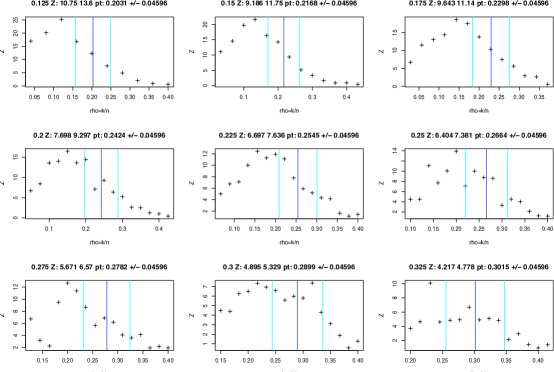
Figure 18. $Z$-scores for suite 12, $N=200$ plotted versus $\rho=k/n$ at each value of $\delta=n/N$. Vertical bars indicate asymptotic phase transition and nominal width of the transition zone.

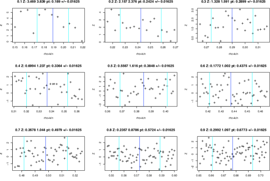
Figure 19. $Z$-scores for suite 12, $N=1600$ plotted versus $\rho=k/n$ at each value of $\delta=n/N$. Vertical bars indicate asymptotic phase transition and nominal width of the transition zone.

Suite 16 is adequately explained, since the standard deviation is fairly close to 1.00 at each $N$.

In all suites the residual standard deviation is decreasing with $N$, and in every case the residual standard deviation is less than 1.10 at $N=1600$. In our view this, together with the structure of the scaling model, merits the conclusion that these random matrix ensembles agree with the Gaussian ensemble for large $n$.

However, there is noticeable structure at small $n$. The key pattern visible in the table is the tendency of residuals to be positive at small $n$.

Some further structure is visible in the $\delta$ variable; figures 16 and 17 show that at $N=200$ there is a dramatic ’blowup’ in variance at small $\delta$, which has largely disappeared at the larger problem size $N=1600$. They also show that suite 16 is already well-behaved at $N=200$, and the ”variance blowup” is largely a phenomenon of suites 11 and 12. Finally, at $N=1600$ one can see indications of curvilinear structure, so evidently the hinged model can only be regarded as an approximation.

As it turns out, the ”variance blowup” is not a variance phenomenon at all; it is caused by significant unmodeled structure in the means as a function of $\rho=k/n$. Figure 18 shows the $Z$-scores at suite 12, for problem size $N=200$. The $Z$-scores are quite large and nonrandom, indicating significant unmodelled structure.

On the other hand, this unmodeled structure is largely a phenomenon of small problem size. Figure 19 shows the $Z$-scores at suite 12, now for problem size $N=1600$. The $Z$-scores are not so large and much more random, indicating that unmodelled structure is less of a problem, except at small $\delta$.

The unmodelled structure can be largely accounted for as a displacement of the $LD50$ by about 1 transition width at $N=200$. The asymptotic phase transition is at $\rho(\delta;Q)$; if we assume that in suite 12 the $LD50$ is not at $\rho(\cdot;Q)$ but instead at $\rho^{\dagger}=\rho(\delta;Q)-w(\delta;N,Q)$, and we assume a probit link, we can expect the $Z$-scores to have a mean

$$\mu\propto\phi((\rho-\rho^{\dagger})/w)/w,$$

where $\phi$ denotes the standard Gaussian density.

Figure 20 fits this model to the $Z$-scores at suite 12, for sample size $N=200$. It accounts for most of the structure in the $Z$-scores at these values of $\delta$.

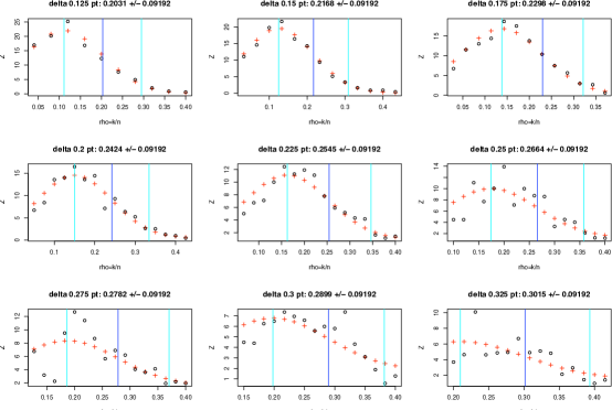
Figure 20. $Z$-scores for suite 12 plotted versus $\rho=k/n$ at 9 different values of $\delta=n/N$, together with fitted mean shift model. Red Crosses portray the displaced $LD50$ model.

5.7.3. Understanding the exceptional ensembles

When $N$ is small and $\delta$ is small, the exceptional ensembles have $LD50$’s displaced substantially below the asymptotic phase transition, It also seems that if we keep $\delta$ fixed and increase $N$, such displacement eventually disappears.

It seems to us that one can understand this phenomenon as a transient effect of random sampling in discrete structures. To explain this, note that when ”success” is declared in our computations, this means that the image of a specific $k$-face $F$ of the polytope $Q$ ‘survives’ projection under $A$, i.e. $AF$ is a face of $AQ$. (Here of course $Q$ is either $T^{N-1}$ or $C^{N}$, see the main text; and the preceding statement deserves and requires rigorous proof; it receives such proof in our other papers). In particular that there is no pair $(x_{0},x_{1})$ both in $F$ with $Ax_{0}=Ax_{1}$. But then there is no vector $v$ supported on those $k+1$ sites with $Av=0$.

On the other hand, if there exist vectors supported on $k+1$ sites that belong to this null space, then there definitely will be $k$-faces $F$ that get lost under projection.

Let $E_{k,n,N}$ denote the event that there exist $k+1$-sparse vectors in the null space of $A$. Then when event $E_{k,n,N}$ occurs there will be a $k$-face of $Q$ that does not survive projection.

For a Gaussian random matrix $A$, with probability one the columns of $A$ are in general position, and so $P(E_{k,n,N})=0$ provided $k<n$. However, for the exceptional ensembles $P(E_{k,n,N})>0$ even for quite small $k$.

The Ternary (1/10) and Expander (1/15) ensembles generate highly sparse matrices $A$. Particularly when $n$ is small, we have observed that these can have sparse solutions in their null space; that is, $E_{k,n,N}$ can have substantial probability.

It may help some readers to know we are effectively discussing the sparsity of the sparsest vector in the null space of $A$; this is often denoted $spark(A)$ (Donoho & Elad, 2003). For Gaussian random matrices $A$, $spark(A)=n$, while for the Ternary and Expander ensembles, we find that $spark(A)$ has a good chance of being much smaller than $n$.

Dossal et al. (2009) have proposed a greedy algorithm which can be used to find sparse vectors in the null space of a matrix. It provides an heuristic upper bound $spark^{+}(A)$ on the spark of a matrix . Applying this algorithm to random draws of Ternary (1/10) and Expander (1/15) we observe sparse vectors satisfying $Az=0$; ranges of these observed sparsity levels are recorded in columns 2 and 3 of table 10.

The sparsity levels recorded in columns 2 and 3 of table 10 indicate clearly that $E_{k,n,N}$ can occur for quite small $k$, but they do not indicate the size of $P(E_{k,n,N})$ or give any other information about the prevalence of these sparse null space vectors. Columns 4-9 of table 10 indicate the empirical bound $spark^{+}(A)$ for suites 1-2,11-12,15-16 with $S/M$ closest to 50%. For Ternary (1/10) with $N=200$ and $n\leq 60$ it is common to draw matrices which contain a column of all zeros, allowing for 1-sparse vectors in the null space. In such cases, $spark(A)=1$, which is dramatically smaller than $n$, what we would see with the Gaussian ensemble.

With such easy counterexamples to uniqueness it now seems remarkable that the typical case, as measured by the observed $LD50$, is as high as we observed. This may be explained by the fact that typically, the bad $k$-sets do not intersect the particular $k$-set we are interested in (i.e. the one supporting the solution of interest).

For the Expander ensemble with $N=200$ and $n\leq 40$ there are vectors in the null space with only 6 nonzeros, and null space vectors with more than 6 nonzeros become common; as a consequence, it becomes increasingly common that of the $M=200$ problem instances presented to (P1) and (LP) for each value of $k$ moderately larger than 6 there will be vectors $x_{1}$ which are sparser than $x_{0}$ and yet which satisfy $Ax_{1}=Ax_{0}=y$.

We observe that the $LD50$ for suites 15-16 is significantly displaced below the asymptotic value for this range of $(N,n)$. Suites 15-16 are observed to have similar values of $LD50$ for this range of $(N,n)$. Although these $LD50$s are similarly displaced, the effect is more noticeable in the $Z$-scores of suite 15 due to its being compared with suite 1 which has a markedly higher $LD50$ than does suite 2 (which suite 16 is compared against).

$(N,n)$	Ternary (1/10)	Expander	1	2	11	12	15	16
(200,20)	1	1	5	4	2	1	2	1
(200,30)	1	5-14	9	7	5	4	3	3
(200,40)	1	6-20	13	10	11	8	9	8
(200,50)	1	19-34	19	14	16	12	17	13
(200,60)	1-61	16-41	25	18	23	16	22	18
(1600,160)	1-61	1-61	39	30	38	29	40	31

Table 10. Sparse vectors in $Nullspace(A)$. Columns 2 and 3 of table 10 indicate minimal sparsity levels of vectors $z$ obeying $Az=0$ with $A$ drawn from ensembles Ternary (1/10) and Expander (1/15). Columns 4-9 indicate the value of the empirical upper bound $spark^{+}(A)$ for suites 1-2,11-12,15-16 with $S/M$ closest to 50%.

If we keep $n/N$ and $k/n$ constant, and $k/n$ small, but let $N$ increase it seems that the probability $P(E_{k,n,N})$ tends to zero rapidly. For $N=1600$ and $\delta=0.1$, the observed $LD50$ values for these exceptional ensembles are within 1 of those observed for the Gaussian suites. We also observe that for $N=1600$ and $n=160$ we are unable to find null space vectors with fewer than $161$ nonzeros. This suggests the following interpretation of what is happening: for each $(\delta,\rho)$ there is a transient effect, such that as $N$ increases, initially it is most likely that $spark(A)$ is less than $\rho\cdot n$, but for sufficiently large $N$, it becomes likely that $spark(A)\approx n$.

Under our interpretation, the driving effect behind the exceptional ensembles is the phenomenon that for small $N$ the matrix $A$ has its columns not in general position; and, for fixed $\delta=n/N$ the chance of observing this phenomenon decays rapidly with increasing problem size $N$.

5.8. Validation ensembles: Rademacher and Hadamard

The computer runs reported here took place over a substantial interval of calendar time. As it happens, two of the matrix ensembles – Rademacher and partial Hadamard – were completed long after the others and the data were not available at the time of the analyses reported so far.

A basic principle in science is out-of-sample validation, namely building a model using data available at a certain moment in time and then later using data that were not available to the model construction to test the model construction.

The fresh data provided by the Rademacher and partial Hadamard runs provide an excellent opportunity for validation of our fitted models.

Such validation could be helpful for the following reason. A critic of our analysis could point out that we have used the same data to choose the decay exponent $\gamma=1/2$ in our scaling model $\mu\sim N^{-1/2}$, as well as to study lack of fit of that model. This is not inferentially rigorous, as the exponent has specifically been chosen to minimize lack of fit, and we then argue that the lack of fit at such $\gamma$ is not significant. The use of the same data for both tasks means that the $t$-scores and $p$-values no longer have the assumed distributions.

In our case, we have about 10,000 $Z$-scores, and we believe this criticism is not as serious as in many other occurrences of this practice, and we are prepared to argue this point. However, in this instance because we have an independent set of validation data, we can actually perform direct model validation and avoid lengthy rationalizations of our earlier analysis.

The validation data have one oddity: The Hadamard ensemble is computable only for special choices of $N$, and we happen only to have data for $N=256$ and $N=512$, while for the Rademacher ensemble we have data for $N=200$, $400$, and $1600$ as per usual.

We now use those data to validate the following points in our analysis.

• Bulk distribution of $Z$-scores;

• Fit of $N^{-1/2}$ model for scaling of means;

• Lack of Fit at small $\delta$ caused by displacement of the LD50.

It will turn out that the Rademacher ensemble is not exceptional while the Hadamard is; and for both Rademacher and Hadamard the models developed using the other ensembles fit rather well.

5.8.1. Bulk distribution of $Z$-scores

In figures 21 and 22 we present a sequence of QQ plots showing the bulk distribution of $Z$-scores for suites $19-20$ (at $N=200$, $400$ and $1600$) and for suites 13-14 (at $N=256$ and $512$). In each plot the identity line is also displayed; if the $Z$-scores had truly a standard normal distribution, they would oscillate around this line.

The Rademacher suite $Z$-scores are typical of what we have already seen in suites 3-10. Recall that $Z$-scores are expected to cluster around the line $Y=X$ at the null hypothesis. There is some noticeable bulk misfit at $N=200$, less at $N=400$, and by $N=1600$ the visual misfit has mostly disappeared. The misfit at $N=200$ is mostly in the lower tail, and in a downward shift away from the $Y=X$ line, meaning that there are situations where our realization of the Rademacher ensemble at $N=200$ gives noticeably better success probabilities than the Gaussian ensemble, and it also gives slightly better success probabilities on average.

The Hadamard suite $Z$-scores are typical of what we have already seen in suites 11,12, and 15. There is some very noticeable bulk misfit at $N=256$, and much less at $N=512$. We do not have data at larger $N$. The misfit at $N=256$ is mostly in the upper tail, meaning that there are some situations where the Hadamard ensemble at $N=256$ gives noticeably worse success probabilities than the Gaussian ensemble. This upper tail effect has mostly disappeared by $N=512$, however for the suite with positive coeficients at $N=512$ we see that the slope of the $Z$-score graph is higher than 1, so the bulk distribution of $Z$-scores has seemingly higher standard deviation than 1.0. This is a sign of overdispersion, i.e. the underlying success probability $p_{1}$ might best be treated as a random variable which varies from realization to realization, but which has the correct expectation $p_{0}$.

Figure 21. $Z$-scores for suites 19-20, the Rademacher ensemble, at $N=200$, $400$ and $1600$

Figure 22. $Z$-scores for suites 13-14, the Hadamard ensemble, at $N=256$ and $512$

5.8.2. Linear models of the $Z$-scores

Above we reported fits explaining the observed $Z$-scores using two models of the form (5.7)-(5.8). We considered two such models, one with the restrictions $\alpha_{0}=0$ and $\beta_{0}=0$, and one without.

The display below shows the output of the $R$ linear model command for the restricted model. The symbol de denotes $\delta-1/2$ and the symbol probSize denotes $1/\sqrt{N}$. The output lists interaction terms such as probSize:de, which is what we have called $\beta_{1}(N)$.

Call:
lm(formula = Z ~ probSize * de + probSize * dea2 - de - dea2 - 1)

Residuals:
     Min       1Q   Median       3Q      Max
-3.08857 -0.65803  0.04351  0.71908  3.04688

Coefficients:
              Estimate Std. Error t value Pr(>|t|)
probSize        -3.357      1.684  -1.993   0.0466 *
probSize:de      2.640      6.410   0.412   0.6805
probSize:dea2  -71.876     14.293  -5.029 6.17e-07 ***
---
Residual standard error: 1.037 on 756 degrees of freedom
Multiple R-Squared: 0.1641,ΨAdjusted R-squared: 0.1608
F-statistic: 49.49 on 3 and 756 DF,  p-value: < 2.2e-16

We have these key points:

• Scaling with $N$: the mean $Z$-score tends toward zero with increasing $N$.

• Standard deviation $\approx 1$. The standard devation of the residual $Z$-scores is close to 1.

• Hinge terms. The linear trend term is not significant but the hinge term is.

When we fit the unrestricted model, allowing non scaling terms that do not decay with increasing $N$, we see that in fact the only term approaching significance is again the scaling Hinge term.

Call:
lm(formula = Z ~ probSize * de + probSize * dea2)

Residuals:
     Min       1Q   Median       3Q      Max
-3.08564 -0.66130  0.04149  0.71351  3.04902

Coefficients:
               Estimate Std. Error t value Pr(>|t|)
(Intercept)    -0.05629    0.18748  -0.300   0.7641
probSize       -2.19063    4.15678  -0.527   0.5983
de              0.51222    0.71232   0.719   0.4723
dea2            0.03154    1.61315   0.020   0.9844
probSize:de    -7.85130   15.83140  -0.496   0.6201
probSize:dea2 -72.84768   35.45530  -2.055   0.0403 *
---

Residual standard error: 1.038 on 753 degrees of freedom
Multiple R-Squared: 0.1179,ΨAdjusted R-squared: 0.112
F-statistic: 20.12 on 5 and 753 DF,  p-value: < 2.2e-16

The unrestricted model has a worse adjusted $R^{2}$ than the scaling model and does not produce a meaningfully better residual standard deviation. We conclude that the scaling model fits the Rademacher ensemble adequately. Also, since the form of the model and the particular analyses we are presenting were both specified before the data became available, the statistics can be considered inferentially rigorous.

The situation with the Hadamard ensemble is quite different. It belongs with the exceptional ensembles, in the sense that substantial lack of fit is evident, particularly at small $\delta$ and and small $N$. Also, since we have only two values of $N$ – $256$ and $512$ – it is unclear that fitting the linear model will in any way validate scaling.

5.8.3. Lack of fit at the Hadamard ensembles

The Hadamard ensemble displays, at $N=256$, the lack of fit which is familiar to us from the exceptional ensembles 11,12, and 15. Figure 23 displays the behaviour of $Z$-scores as a function of $\rho=k/n$ within each constant-$\delta$ slice, together with fits using the displaced $LD50$ model which we showed described the other exceptional ensembles, with the same displacement of one transition width. Note that this model was developed entirely before these data became available. Hence this display presents a validation of the earlier approach.

One can see in figure 23 that the displaced $LD50$ model indeed adequately describes the structure at small $\delta$ in the Hadamard ensemble at $N=256$. For comparison, we show in figure 24 which demonstrates that no such model is needed in the Rademacher ensemble.

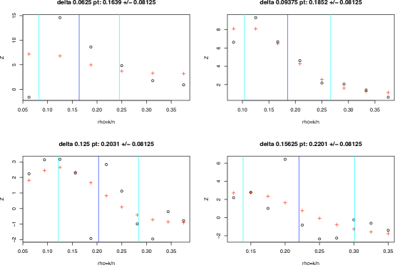
Figure 23. $Z$-scores for suite 14, $N=256$ plotted versus $\rho=k/n$ at each value of $\delta=n/N$. Vertical bars indicate asymptotic phase transition and nominal width of the transition zone. Red Crosses indicate fits using the displaced $LD50$ model developed earlier. This model describes reasonably well the lack-of-fit.

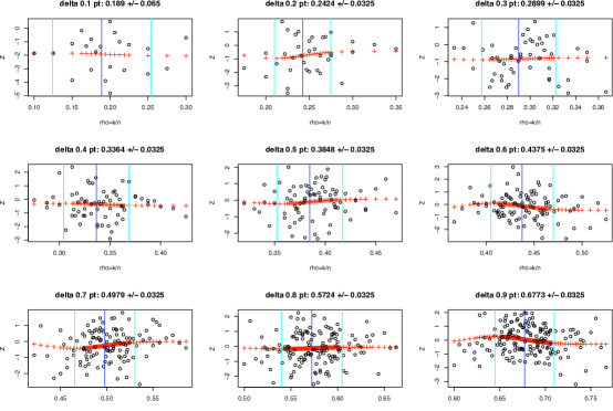
Figure 24. $Z$-scores for suite 20, $N=200$ plotted versus $\rho=k/n$ at each value of $\delta=n/N$. Vertical bars indicate asymptotic phase transition and nominal width of the transition zone. Red Crosses indicate fits using displaced $LD50$ model. This lack of fit is not substantial and the model does not capture any that might be evident.

5.8.4. Implications of the validation ensembles

Our analysis of the validation ensembles follows the script we arrived at in earlier analysis. Since the models being fit – which in earlier analysis depended on the same data as those being explained – now do not depend on the data being explained, we gain additional confidence about the model we developed. In particular, the partitioning into ordinary and exceptional ensembles, the modelling of mean $Z$-scores with power law means having decay $N^{-1/2}$ in ordinary ensembles and the existence of transient effects in exceptional ensembles at small $N$ and $\delta$ – all seem confirmed in our validation ensembles.

5.9. Conclusions

We made extensive computational experiments, solving underdetermined systems of equations $y=Ax$ using linear programming based algorithms in cases where a known solution $x_{0}$ is a $k$-sparse vector, and $A$ is an $n$ by $N$ matrix with $n<N$. We tracked the success of the linear programming algorithms at recovering this known sparse solution.

We considered millions of such systems at a range of problem sizes and covering a range of random matrix ensembles. Our work would have required more than 6 years using a single modern desktop computer.

The Gaussian ensemble is well understood in the large-problem limit based on prior theoretical work. It is known there is a phase transition in the $(\delta,\rho)$ phase diagram at the curve $(\delta,\rho(\delta;Q))$. For $(\delta,\rho)$ below this curve we see success – the probability of success tends to $1$ – and above this curve we see failure – the probability of success tends to $0$. Here $\delta=n/N$ is a measure of matrix shape and $\rho=k/n$ is a measure of sparsity of the solution vector.

Empirical work at the Gaussian ensemble shows that for finite $N$ the location of 50% success closely matches the asymptotic phase transition $\rho(\delta;Q)$. In fact the success probability behaves with $\rho$ as $\bar{\Phi}((\rho-\rho(\delta;Q))/w(\delta,N))$ where $\bar{\Phi}$ denotes the $N(0,1)$ survival function. and $w(\delta,N)$ is a width parameter. In picturesque terms there is a transition zone: for $\rho<\rho(\cdot;Q)-3w$ success is overwhelmingly likely; for $\rho>\rho(\cdot;Q)+3w$ success is overwhelmingly unlikely, and in between there is a transition zone of width $\propto w$. $w$ tends to zero with increasing problem size $N$ as $O(N^{-1/2})$.

Broadly similar behaviour is evident at all but two of the non-Gaussian matrix ensembles considered here. Hence, the evidence points to asymptotic phase transitions at the conforming matrix ensembles which are all located at precisely the same place as in the Gaussian case. This is the hypothesis of weak universality advanced and maintained in the main text.

The above conclusions emerged from using standard two-sample statistical inference tools to compare results from non-Gaussian ensembles with their Gaussian counterparts at the same problem size and sparsity level. We considered the behaviour of over 16,000 $Z$-scores and observed good bulk agreement of the two-sample $Z$-scores with the $N(0,1)$ distribution, supporting the null hypothesis of no difference; however, fitting a linear model to an array of such $Z$-scores we were able to identify statistically significant nonzero mean $Z$-scores varying with problem size, with undersampling fraction $\delta=n/N$, and, at small $\delta$, with $\rho$. The means exhibit trends varying from ensemble to ensemble, but they decay with problem size $N$ as $O(N^{-1/2})$. The nonzero means are consistent with weak, ‘asymptotic’, universality but not with strong, finite-$N$, universality. After accounting for these means, the $Z$-scores exhibit standard deviations close to one, with a small fraction of exceptions.

For the non-Gaussian ensembles studied here the fact that phase diagram behaviour matches the Gaussian case goes far beyond current theory (e.g. Adamczak et al. (2009) )