Stabilizing Hadron Resonance Gas Models against Future Discoveries

Abstract

We examine the stability of hadron resonance gas models by extending them to take care of undiscovered resonances through the Hagedorn formula. We find that the influence of unknown resonances on thermodynamics is large but bounded. Hadron resonance gases may be internally consistent up to a temperature higher than the cross over temperature in QCD; but by examining quark number susceptibilities we find that their region of applicability seems to end substantially below the QCD cross over. We model the decays of resonances and investigate the ratios of particle yields in heavy-ion collisions. We find that observables such as hydrodynamics and hadron yield ratios change little upon extending the model. As a result, heavy-ion collisions at RHIC and LHC are insensitive to a possible exponential rise in the hadronic density of states, thus increasing the stability of the predictions of hadron resonance gas models in this context.

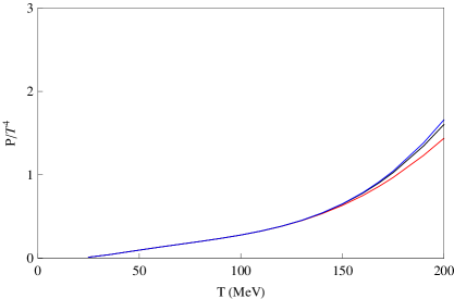
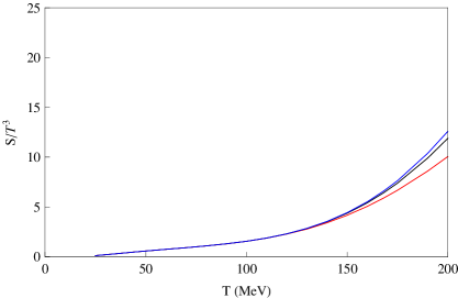
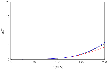
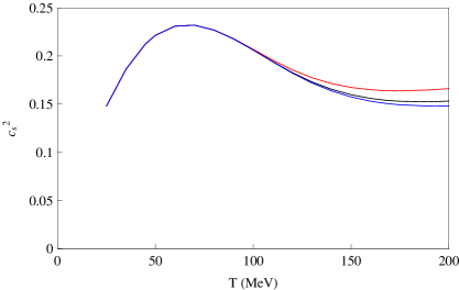
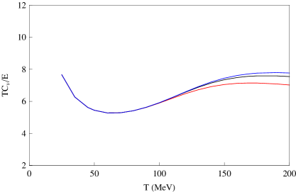
Figure 1: Thermodynamic quantities in the hadron resonance gas variant which we call HRG1. As the mass cutoff, $\Lambda$ on the states included in the model is changed the predictions change monotonically. These are results at zero chemical potential.

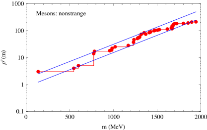
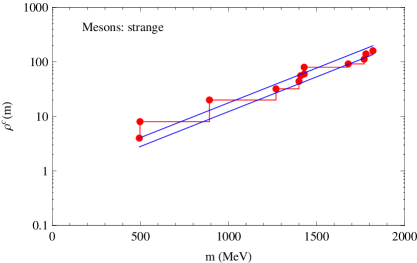
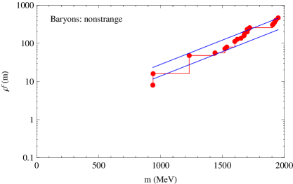
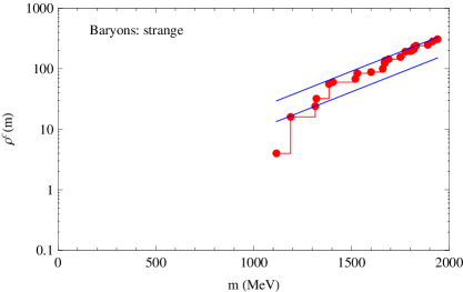
Figure 2: Fit of the parameters of the Hagedorn spectrum to states from the particle data book for masses up to 2000 MeV. The band is wide enough to include all but the two extreme points in the cumulative distribution for each of four classes of hadrons.

Hadron resonance gas models (HRGM) in their modern form were first explored in dixit ; suhonen ; greiner ; heinz , where the emphasis was on exploring the phase diagram. Then, following the CERN SPS experiments with heavy-ions, it was found that integrated particle yields could be explained in HRGMs bms ; yen ; becattini . Typically, one defines the thermodynamics of HRGMs through the summed free energy—

$$\log Z(V,T,\mu)=\int dm\left[\rho_{M}(m)\log Z_{b}(m,V,T,\mu)+\rho_{B}(m)\log Z_{f}(m,V,T,\mu)\right],$$ (1)

where the gas is contained in a volume $V$, has temperature $T$ and chemical potential $\mu$, $Z_{b}$ is the partition function for an ideal gas of bosons with mass $m$, $Z_{f}$ of an ideal gas of fermions, $\rho_{M}(m)$ is the spectral density of mesons, and $\rho_{B}(m)$ of baryons. From this one computes the energy density, $E$, by taking a derivative with respect to $1/T$, and the pressure, $P$, by taking a derivative with respect to $V$. One can also find the conformal symmetry breaking measure $(E-3P)/T^{4}$, the entropy density, $S/T^{3}=(E+P)/T^{4}$, the speed of sound, $c_{s}^{2}=dP/dE$, and the specific heat, $c_{\scriptscriptstyle V}$.

Hadron properties enter these models through $\rho_{B,M}$ and the treatment of the decay width and size of the hadron. We follow becattini in neglecting an excluded volume effect for hadrons, i.e., we treat the hadrons as effectively point-like. In constructing the thermodynamics, the decay width is usually neglected; we accept this assumption through the part of this work which deals with the equation of state, but, as usual, include decays when we explore other aspects of HRGMs. One aspect common to models of the type explored in bms ; yen ; becattini is to take the observed spectrum of hadrons up to some cutoff $\Lambda$, i.e., write

$$\rho_{M,B}(m)=\sum_{i}^{m_{i}\leq\Lambda}g_{i}\delta(m-m_{i}),$$ (2)

where $m_{i}$ are the masses of the known hadrons and $g_{i}$ the degeneracy factor $(2J_{i}+1)(2I_{i}+1)$ where $J_{i}$ is the spin and $I_{i}$ the isospin, and the sum is over meson or baryon states, as appropriate. We call such models HRG1. We include in the sum above all the states which are reasonably well established, and labeled as better than 1 star in the particle data book.

Clearly the predictions of thermodynamic quantities in HRG1 depend on the mass cutoff $\Lambda$. This is shown in Figure 1. Even at temperatures as low as 150 MeV, there is a 5% increase in the energy density when $\Lambda$ is increased from 1600 MeV to 1800 MeV, and a further 2% increase when it is increased to 2000 MeV. Changes at temperatures of 170 MeV or so are significantly larger. Predictions of quantities such as the speed of sound, $c_{s}^{2}$, and the specific heat, $c_{\scriptscriptstyle V}$, are significantly less stable. Recent quark model qmod and lattice computations lat lead us to believe that there is a much higher density of hadronic states in the mass range 2–3 GeV than below 2 GeV. If so, it is not clear by how much the predictions will change as $\Lambda$ is increased to 3 GeV or beyond.

In order to explore the stability of predictions from HRGMs, we develop a variant of these models in which we take the observed spectrum of states up to a certain cutoff $\Lambda$, as before, and above this we put in an exponentially rising cumulative density of hadron states in hagedorn ; frautschi . It is well known that such a density of states overcomes the exponential suppression of higher mass resonances in eq. (1). As a result, there is a limiting temperature in these models, which was, long ago, taken as evidence of a QCD phase transition cabibbo . So, the extended model, HRG2, has

$$\rho_{h}(m)=\sum_{i}^{m_{i}\leq\Lambda}g_{i}\delta(m-m_{i})+\frac{a_{h}}{T_{H}}{\rm e}^{m/T_{H}}\Theta(m-\Lambda),$$ (3)

where the model parameters $T_{H}$ and $a_{h}$ are fitted to data on the cumulative distribution of different sets of hadrons, $h$. Similar models have been used to study observables as diverse as dilepton production ruuskanen to chemical equilibration shovkovy . A comparison of the equation of state with different density of states for the Hagedorn spectrum is presented later.

Class ($h$)	$a_{h}^{\rm min}$	$a_{h}^{\rm max}$
Mesons (non strange)	0.81	1.64
Mesons (strange)	0.64	0.94
Baryons (non strange)	0.73	1.47
Baryons (strange)	0.50	1.10

Table 1: The extreme values of $a_{h}$ such that for $T_{H}=340$ MeV the cumulative density of hadron states up to 2000 MeV lies within the bands except for the two extreme points on each side.

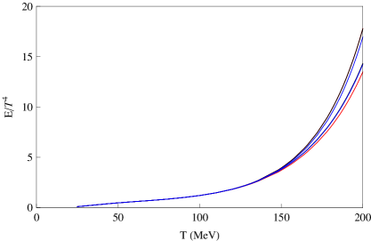
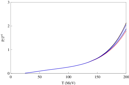
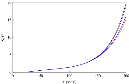
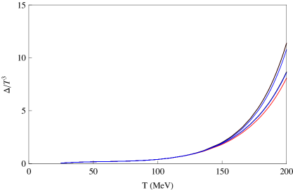
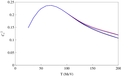
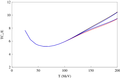
Figure 3: Thermodynamic quantities in the hadron resonance gas variant which we call HRG2. At each value of the parameter $\Lambda$, there are upper and lower limits on every thermodynamic quantity. The predictions of HRG2 are stable, since the allowed band shrinks as $\Lambda$ increases, and the band for higher $\Lambda$ is entirely contained inside that for a lower $\Lambda$. If QCD has a cross over at finite temperature, and the same equation of state is valid on both sides, then $c_{s}^{2}$ falls monotonically across this point, and the softest point is not at $T_{c}$.

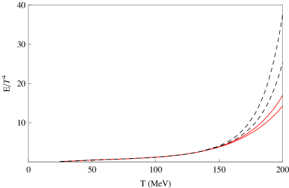
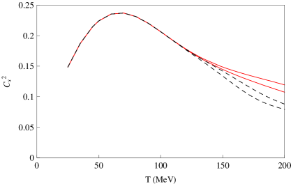
Figure 4: Comparing predictions of thermodynamics using HRG2 with the parametrisation of eq. (3) (full line) and eq. (4) (dashed line). The uncertainty bands of all quantities overlap over the range of temperatures of interest.

We perform fits separately to non-strange mesons, strange mesons, non-strange baryons and strange baryons. All states in the particle data book with rating higher than 1 star and mass up to 2000 MeV are used in these fits. The quantity $T_{H}$ is obtained by a global fit to all four types of hadrons, whereas we fit upper and lower values for $a_{h}$ for each class of hadrons. We have allowed the band of $a_{h}/T_{H}$ to be wide enough that all but two of the extreme high and low points are within the band. The goodness of such fits can be gauged from Figure 2. The fitted parameter sets to be used in eq. (3) are given in Table 1. Note that the best fit value of $T_{H}$ is significantly higher than $T_{c}$, the cross over temperature of QCD jaipur . This is not unexpected, since there is good evidence that $T_{H}$ and $T_{c}$ are not equal, at least at finite $N_{c}$ bringolz . As a result, the model in eq. (3) is internally consistent well beyond $T_{c}$.

Using this extended model, we get the predictions of thermodynamic quantities shown in Figure 3. Note that for each value of $\Lambda$ there is an upper and lower limit to the prediction for any thermodynamic quantity, one from the maximum and the other from the minimum of the $a_{h}$. As one changes $\Lambda$, the band for higher $\Lambda$ lies entirely within that for lower $\Lambda$. This pleasant property implies a stability of the predictions of the HRG2 model for bulk thermodynamic quantities. Even for $c_{s}^{2}$ and $c_{\scriptscriptstyle V}$, predictions of HRG2 are stable in this sense up to a temperature of 160 MeV. The allowed band at 150 MeV is about 2–7% for $\Lambda=2000$ MeV.

A different density of states for the Hagedorn model has also been used in the literature ranft ; polish . The density of states in the HRG2 with this change would be

$$\rho_{h}(m)=\sum_{i}^{m_{i}\leq\Lambda}g_{i}\delta(m-m_{i})+\frac{c_{h}}{(m^{2}+m_{0}^{2})^{5/4}}{\rm e}^{m/T_{H}}\Theta(m-\Lambda).$$ (4)

Typically this model is used with $m_{0}=500$ MeV. We have used this canonical value as well $m_{0}=250$ MeV and 1000 MeV. Note that in the limit as $m_{=}0\to\infty$, this model reduces to the one in eq. (3). The best fit value of $T_{H}$ changes significantly as we vary $m_{0}$, being 210 MeV for the central value of $m_{0}$, and sliding up to 250 MeV as $m_{0}$ changes to 1000 MeV. The quality of fit improves marginally as $m_{0}$ increases, being best for the density of states in eq. (3). The uncertainty in the value of the derived hadronic quantity, $T_{H}$, is closely related to the fact that a string model of hadrons is not a unique and self-consistent theory. As a result, the pre-exponential factor can be tweaked at will, resulting in large possible changes to the string tension, or, equivalently, to $T_{H}$.

Using $m_{0}=500$ MeV and $T_{H}=210$ MeV, we take as the allowed band of $c_{h}$ a definition analogous to that used in Table 1. This gives us the uncertainties in the corresponding predictions of thermodynamic quantities. As one could guess, the pleasantly stable results for thermodynamics shown in Figure 3 are model artifacts. In Figure 4 we show that the uncertainty bands in the two models defined by eqs. (3, 4) exclude each other in the vicinity of $T=170$ MeV. In view of these uncertainties, we do not consider the more detailed models which have been used polish . In future, when observations of the hadron spectrum are extended to significantly larger masses, a more detailed consideration of string models may become a fruitful topic of research.

Lattice computations of the equation of state give $E/T^{4}=1.4\pm 0.2$ at a temperature of 140 MeV jaipur . At such low temperatures the known hadron spectrum dominates the results (see Figure 4). The mismatch between lattice and hadron gas models is due to the fact that current day lattice thermodynamics computations are performed on lattices which are too coarse at such low temperatures. The best lattices have cutoff of around 1100 MeV when doing thermodynamics at $T=140$ MeV. Since the cutoff is comparable to the low-lying baryon masses, the hadron resonance spectrum is strongly disturbed and the low-temperature results are not yet physical. Since the lattice spacing varies inversely with the temperature, lattice results at higher temperatures are expected to be reasonable. The efficacy of the lattice closer to $T_{c}$ is borne out by the fact that renormalization group invariant estimates of $T_{c}$ are possible with the cutoffs in use today scaling . Interestingly, present day lattice computations at a temperature of 210 MeV give $E/T^{4}=12.4\pm 0.3$ jaipur , which is also below the prediction of HRG2. However, as shown in Figure 4, at this temperature the problem very likely lies with the hadron gas models. We demonstrate this next.

A phase transition involves a singularity in the free energy. As a result one usually does not have the same elementary excitations in terms of which the thermodynamics is constructed on both sides of a phase transition. However, there is no singularity of the free energy at a cross over. As a result, there is no theoretical bar to a model which is valid on both sides of the cross over. One way to investigate the applicability of such models on both sides of $T_{c}$ is to look at quantum number susceptibilities (QNS). Introduce chemical potentials for the three quantities conserved in strong interactions, namely the baryon number, the third component of the isospin ($I_{3}$) and the strangeness. Then the baryon number susceptibility is defined to be

$$\chi_{B}(T)=\left.\frac{\partial^{2}P(T,\mu_{B},\mu_{I_{3}},\mu_{S})}{\partial\mu_{B}^{2}}\right|_{\mu_{B}=\mu_{I_{3}}=\mu_{S}=0}.$$ (5)

This defines the susceptibility at zero chemical potential, since there is lattice data on this quantity, although, of course, it may also be taken at finite chemical potential. Following nls the non-linear susceptibilities (NLS) are defined as

$$\chi_{B}^{(n)}(T)=\left.\frac{\partial^{n}P(T,\mu_{B},\mu_{I_{3}},\mu_{S})}{\partial\mu_{B}^{n}}\right|_{\mu_{B}=\mu_{I_{3}}=\mu_{S}=0}.$$ (6)

The QNS is just the NLS for $n=2$. In exact analogy one can also define strangeness susceptibilities and so-called off-diagonal susceptibilities where some of the derivatives are with respect to one chemical potential and others with respect to another strange . The QNS predicted by HRG1 and HRG2 are shown in Figure 5. The enhanced density of baryon states in HRG2 leads to a substantial increase in $\chi_{B}(T)$. As expected, current lattice data gg ; bi does not match these curves.

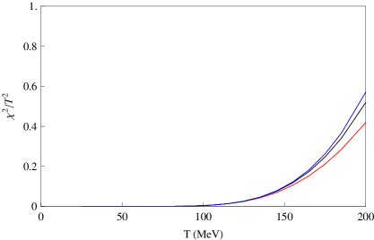
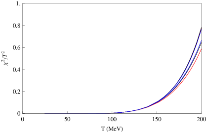
Figure 5: The baryon number susceptibility computed in hadron resonance gases. The first panel gives the results in HRG1 and the second in HRG2. The colour coding is the same as in previous figures. Note the importance of including the Hagedorn spectrum of baryons.

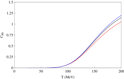
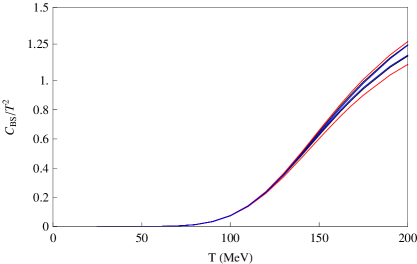
Figure 6: $C_{BS}$ in the hadron resonance gas models HRG1 (left) and HRG2 (right). One expects $C_{BS}$ to be a monotonic function of temperature in a resonance gas model.

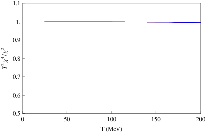
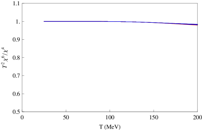
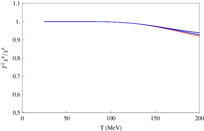
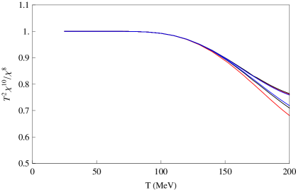
Figure 7: The non-linear baryon number susceptibilities computed in hadron resonance gas model HRG2. We have plotted the ratios $\chi^{(n+2)}T^{2}/\chi^{(n)}$ for $n=2$, 4, 6 and 8. The colour coding is the same as in previous figures. The results are very stable against the mass cutoff.

The reason is very accurately probed by the quantity

$$C_{BS}=-3\frac{\chi_{BS}(T)}{\chi_{S}(T)},$$ (7)

where $\chi_{BS}(T)$ is one of the off-diagonal QNS koch ; linkage . The normalization is such that $C_{BS}=1$ in an ideal gas of quarks. The HRG1 and HRG2 predictions of $C_{BS}$ are shown in Figure 6. Since the lowest mass baryons are non-strange, $C_{BS}$ must start at zero. It is seen to climb monotonically with temperature. $C_{BS}$ can exceed unity if the contribution of the singly and doubly strange baryons to $\chi_{B}$ exceeds half the contribution of strange mesons to $\chi_{S}$. Since the strange meson spectrum starts at a much lower mass than the strange baryon sector, this cannot happen at low temperature. However, as seen in Figure 2, the observed density of strange baryons grows much more rapidly with temperature than that of strange mesons. As a result, at sufficiently high temperature $C_{BS}$ exceeds unity. In HRG2 $C_{BS}$ remains above unity until $T_{H}$. Hence there is no continuity between this model and the physics of the high temperature phase of QCD.

The ratios of successive NLS in the HRG2 is shown in Figure 7. These ratios are not very sensitive to the change from HRG1 to HRG2. Note that they are extremely constant as a function of temperature. In contrast, lattice computations show much structure in the vicinity of $T_{c}$ as a consequence of the nearness of the QCD critical point gg . The hadron resonance gas, being a mixture of ideal gases, sees no critical point, but only the Hagedorn limiting temperature. As a result, it misses all this structure.

We have shown here that there are major points of mismatch between lattice computations of QNS and the resonance gas models for $T>T_{c}$. Since there is no phase transition in QCD at $\mu_{B}=0$ but only a crossover, the failure of a model soon above $T_{c}$ also implies its failure a little before $T_{c}$. This means that the resonance gas models are restricted in their range of applicability to well below $T_{c}$. In this real QCD seems to be very different from either pure gauge theory or large-$N_{c}$ QCD, where the resonance gas model could remain perfectly accurate right up to the first order phase transition in these models. We turn next to the question of whether heavy-ion observables can give information on the Hagedorn spectrum of resonances.

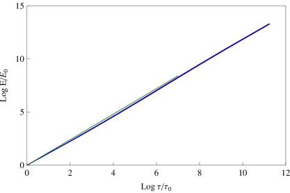
Figure 8: Bjorken flow in the hadron resonance gas phase starting from an initial energy density of 1 GeV/fm³, with the bands of uncertainty corresponding to $\Lambda=1600$ MeV, 1800 MeV and 2000 MeV for $c_{s}^{2}$. Also shown (in green) is the flow for constant $c_{s}^{2}=1/5$. There is very little difference between these flows.

One of the uses to which equations of state can be put is hydrodynamics. We perform the following simple computation with the HRG2 equation of state— use it to evolve a longitudinally expanding fireball which has cooled to a point where its energy density, $E$, is 1 GeV/fm³. For longitudinal flow, the quantity $E/E_{0}$ is a function only of the ratio $\tau/\tau_{0}$ where $\tau$ is the proper time, and $\tau_{0}$ the initial time, when $E(\tau_{0})=E_{0}$. We integrated the longitudinal flow equation with upper and lower band of $c_{s}^{2}$ for $\Lambda=1600$ MeV, 1800 MeV and 2000 MeV. We found that the effect of these changes is minimal, as we show in Figure 8. For comparison we also show the flow obtained with constant $c_{s}^{2}=1/5$. This is almost indistinguishable from the other flows. Similarly, the result of a computation with the density of states in eq. (4) is indistinguishable from these. So, hydrodynamics is almost blind to the level of detail in the equation of state that we have studied.

The main phenomenological application of hadron gas models, however, is in the analysis of particle yields in heavy-ion collisions. Most of the particle species observed in the detector are those which are stable under strong interactions, because the others decay long before reaching the detectors. The computation of the yield of particles in a hadron gas model is matched to data to extract the reaction volume and freezeout temperature and chemical potentials bms ; yen ; becattini .

In HRG1 one creates a table of decays from the particle data book. Each hadron $H_{i}$ has decay modes labeled by $\alpha$. The reaction

$$H_{i}\to\sum_{j}n^{\alpha}_{ij}H_{j}$$ (8)

proceeds with a branching fraction $B_{i}^{\alpha}$, where $n_{ij}^{\alpha}$ is the number of hadrons $H_{j}$ produced in this reaction. For later convenience we add the trivial rule that stable particles decay to themselves with branching ratio unity. The expected number of $H_{j}$ produced per decay of $H_{i}$ are

$$N_{ji}=\sum_{\alpha}B_{i}^{\alpha}n_{ij}^{\alpha}.$$ (9)

For a stable particle $H_{i}$, we have $N_{ii}=1$ and $N_{ji}=0$ for all other $j$. In general, some of the decay products, $H_{j}$, may be unstable under strong interactions; in that case one has to follow the decay chain until only stable particles remain. The expected number of $H_{j}$ resulting from $H_{i}$ after all this, ${\cal N}_{ji}$, is easily found by sufficient number of matrix multiplications—

$${\cal N}_{ji}=\sum_{k_{1},k_{2},\cdots,k_{m}}N_{jk_{1}}N_{k_{1},k_{2}}\cdots N_{k_{m},i},\quad i.e.\quad{\cal N}=N^{m}.$$ (10)

The minimum power $m$ to which the matrix $N$ has to be raised is equal to the maximum number of steps in any decay chain. From the formula above it is clear that the rows of the matrix $\cal N$ which correspond to unstable hadrons are zero. This means that ${\cal N}={\cal N}N$, and hence if $m$ is chosen to be larger than actually required, the cost is in CPU time and not in correctness. Proofs of all these assertions can be written down most simply by noting the structure of the matrix $N$, but insight is also gained by examining a one-to-one correspondence between this problem and problems on directed graphs graph . Finally, the expected yield of a stable particle, $H_{j}$, resulting from a fireball which freezes out at temperature $T$ and chemical potentials $\mu$ is

$$N_{j}(V,T,\mu)=\sum_{i}^{m_{i}<\Lambda}{\cal N}_{ji}N^{\rm th}_{i}(V,T,{\mu}),$$ (11)

where $N_{i}^{\rm th}$ is the number of $H_{i}$ in thermal equilibrium. From this, it is clear that for hadron yield computations, it not necessary to keep track of the detailed decays of every $H_{i}$. It is sufficient to keep ${\cal N}_{ij}$, i.e., the expected number of hadrons $H_{j}$, stable under strong interactions, resulting from the decay of of each $H_{i}$. In any case, the data may be read off the particle data book.

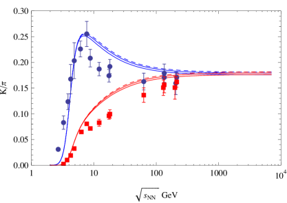
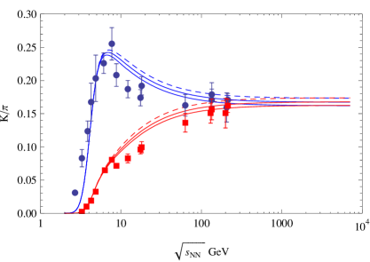
Figure 9: The $K/\pi$ ratio obtained in our models using as input the energy dependence of the freezeout values of $T$ and $\mu$ obtained in andronic by fitting to the data exhibited. The first figure is for decay model 1 and the second for decay model 2. Only the results for $\Lambda=2000$ MeV are shown for clarity.

In HRG2 the yield computation is not so straightforward, since one has to start with a model ${\cal N}_{ji}$ for all $H_{i}$. In this first study we restrict ourselves to models where $H_{j}=\pi$, K or a generic baryon (i.e., we lump the ground-state octet and decuplet baryons into one). As a result, we cannot answer detailed questions about the yield, but only questions of total particle multiplicity and $K/\pi$ or meson/baryon ratios. In general, we expect ${\cal N}_{ji}$ (for fixed $H_{j}$) to depend on the mass of $H_{i}$, so, a generic model for decays is

$${\cal N}_{ji}=a^{j}_{0}+a^{j}_{1}m_{i}+a^{j}_{2}m_{i}^{2}+\cdots.$$ (12)

While ${\cal N}_{ji}$ may well depend on other quantum number of $H_{i}$, we are neither able to confirm or rule this out. Therefore, we decided to work with the simple model above in this paper. The decays of the heaviest hadrons are not yet studied well enough to provide further constraints. Further, incomplete data may contain unknown biases. Hence we neglected the heaviest hadrons and constrained the model with data for hadrons with masses up to 2000 MeV.

Due to the high threshold for the production of a baryon-antibaryon pair, the decays of such particles do not involve such a pair in the final state. Such pairs are rare also in the known decays of hadrons with mass greater than 2000 MeV, being seen mainly in the final state of strange mesons. The branching ratios to such pairs are still mostly ill-measured. As a result, we are unable to make any testable model about the expected occurrence of baryon-antibaryon pairs in decays of the Hagedorn spectrum of resonances. We therefore take the simplest possible model:

$${\cal N}_{Bi}=B_{i},$$ (13)

that the number of baryons in the final state of the decay of any particle is equal to the baryon number of the resonance, $B_{i}$. When better data on resonances between 2000 and 3000 GeV becomes available, the model can be refined by adding higher terms from eq. (12).

The production of $K\overline{K}$ pairs is also strongly suppressed in the decays of hadrons; this is a statement of the OZI rule. Cases which contradict this rule are known, but our attempts to make statistical models of such decays falls on the rock of insufficient data. Thus, we are forced to the rule that

$${\cal N}_{Ki}=S_{i},$$ (14)

the number of kaons produced in the decay of $H_{i}$ is equal to its strangeness, $S_{i}$. We also examined a variant of this rule, which is that the strangeness in the baryon sector percolates down to strange baryons, and does not go into production of kaons. This corresponds to the variant model ${\cal N}_{Ki}=S_{i}(1-\delta_{B_{i},1})$. We refer to this as the decay model 2, to distinguish it from the model in eq. (14), which we call decay model 1.

Finally, we consider the expected number of pions produced in the decays of resonance. We fit the linear model

$${\cal N}_{\pi i}=b+a{\cal M}_{i},$$ (15)

where ${\cal M}_{i}$ is that part of the mass of $H_{i}$ which is available for decay to pions. For unflavoured mesons, the available mass is the mass of the particle, for strange mesons, the available mass is the difference between the mass of a kaon and the mass of $H_{i}$, and for a baryon it is the difference between the mass of $H_{i}$ and a typical baryon mass, which we take to be 1000 MeV. This simple model is fitted to four sets of data— separately for strange and non-strange mesons and baryons. In all these cases we found $b$ consistent with zero and $a\simeq 1.5$ GeV^-1, and consistent with each other. Adding in a term quadratic in masses to the model does not improve the fit significantly, so we keep to the linear model above. It may be useful to note the following implication: out of every GeV of rest mass of the higher resonances, about 500 MeV is available as the kinetic energy of each pion.

This completes the specification of a simple model for the ${\cal N}_{ji}$ in HRG2. Many more refinements and elaborations of the model are possible, however, this model is sufficient for the computations that we exhibit next. We extend the yield formula of eq. (11) to

$$N_{j}(V,T,\mu)=\sum_{i}{\cal N}_{ji}N^{\rm th}_{i}(V,T,{\mu}),$$ (16)

where we use the empirically determined ${\cal N}_{ij}$ for $m_{i}<\Lambda$ and the model for $m_{i}>\lambda$. There are a very small number of baryons whose masses are sufficiently well-known to be included in HRG1, but whose decays are not very well known. For these we used the decay models.

The $K^{\pm}/\pi^{\pm}$ ratios have been determined at AGS ags , SPS sps and RHIC rhic energies. In order to compare with this data we need to take into account the fact that the initial state has no strangeness. Due to strangeness conservation in strong interactions this condition of zero overall strangeness has to be enforced as a canonical constraint, i.e., the $K/\pi$ ratios have to be determined in the canonical ensemble suhonen2 ; pbmrev . We implement this in our computations of hadron yields.

Our results for the $K/\pi$ ratio as a function of the beam energy $\sqrt{S}$ are shown in Figure 9. In this computation we have used the freezeout parameters deduced in andronic . As expected, the ratios of yields are a little higher in decay model 1. Note also that there is a little difference between the predictions of HRG1 and HRG2. For the same freezeout conditions, HRG2 gives a slightly smaller value of the yield ratio. In principle, the freezeout conditions that one deduces from data could be dependent on specifics of the hadron gas model one uses. Our results indicate that this dependence is at best mild. To check this we have implemented the freezeout criterion of freezeout . Using this we find that the freezeout parameters change only marginally from HRG1 to HRG2, consistent both with the conclusions of freezeoutstable and the results in Figure 9. In future we plan a more detailed study of hadron yields, and the effects of the Hagedorn spectrum on the chemical composition at freezeout in baryon rich matter.

We conclude with a summary of our investigation into hadron resonance gas models of the kind which have been used to explain hadron yields in heavy-ion collisions. The thermodynamics of such resonance gases (HRG1) is strongly dependent on the cutoff in the spectrum at temperatures of over 100 MeV. In this paper we have investigated an extension of the hadron resonance gas models in which as yet unobserved resonances are included using the Hagedorn model of the hadron spectrum (HRG2) with two different densities of state (eqs. 3 and 4). We found that the Hagedorn temperature, $T_{H}$, is strongly dependent on details of the model for the hadron spectrum. This implies that the present knowledge of the spectrum of QCD is as yet unable to constrain string models of hadrons.

Each of the HRG2 models stabilizes the uncertainty in thermodynamics below $T_{c}$ due to the cutoff in HRG1. However, the predictions of the two variants of the model are different. While the model is defined up to $T_{H}$, we found that HRG2 gives unrealistic results for thermodynamics, especially for $C_{BS}$, from $T_{c}$ to $T_{H}$. Since there is no phase transition in QCD, a failure of a model near and above $T_{c}$ also implies a failure near and below $T_{c}$. This leads us to believe that the accuracy of resonance gas models cannot be pushed much closer to $T_{c}$ than the freezeout temperature. Of course, this leaves open the interesting possibility that resonance gas models describe the physics of transport that leads to freezeout, for example, the thickness of the freezeout layer.

We also investigated observable quantities in heavy-ion collisions, such as hadron yields. In order to do that, we had to develop a novel model for the decay of Hagedorn resonances. We found that the significant uncertainties that we saw in thermodynamics lead to rather small changes in observables such as the $K/\pi$ yield ratio. This has positive implications on efforts to explain hadron yields from heavy-ion observation.

References

- (1) V. V. Dixit and E. Suhonen, Z. Phys., C 18 (1983) 355.
- (2) J. Cleymans, K. Redlich, H. Satz and E. Suhonen, Z. Phys., C 33 (1986) 151.
- (3) U. Heinz, P. R. Subramanian, H. Stöcker and W. Greiner, J. Phys., G 12 (1986) 1237.
- (4) K. S. Lee, M.-J. Rhoades-Brown, and U. Heinz, Phys. Rev., C 37 (1988) 1452.
- (5) P. Braun-Munzinger, J. Stachel, J. P. Wessels, N. Xu, Phys. Lett., B 365 (1996) 1.
- (6) G. D. Yen and M. I. Gorenstein, Phys. Rev., C 59 (1999) 2788.
- (7) F. Becattini et al., Phys. Rev., C 64 (2001) 024901.
-
(8)
S. Godfrey and N. Isgur, Phys. Rev., D 32 (1985) 189;
S. Capstick and N. Isgur, Phys. Rev., D 34 (1986) 2809. - (9) S. Basak et al., Phys. Rev., D 76 (2007) 074504.
- (10) R. Hagedorn, Nuovo Cimento Suppl., 3 (1965) 147.
- (11) S. Frautschi, Phys. Rev., D 3 (1971) 2821.
- (12) N. Cabibbo and G. Parisi, Phys. Lett., B 59 (1975) 67.
- (13) A. V. Leonidov and P. V. Ruuskanen, Eur. Phys. J., C 4 (1998) 519.
- (14) J. Noronha-Hostler, C. Greiner and I. A. Shovkovy, Phys. Rev. Lett., 100 (2008) 252301.
- (15) S. Gupta, J. Phys., G 35 (2008) 104018, and references therein.
- (16) H. B. Meyer, Phys. Rev., D 80 (2009) 051502.
- (17) S. Gupta, Phys. Rev., D 64 (2001) 034507.
- (18) R. V. Gavai and S. Gupta, Phys. Rev., D 68 (2003) 034506.
- (19) R. V. Gavai and S. Gupta, Phys. Rev., D 73 (2006) 014004.
- (20) B. Bringolz and M. Teper, Phys. Rev., D 73 (2006) 014517.
- (21) R. Hagedorn and J. Ranft, Suppl. Nuovo Cim., 6 (1968) 169.
- (22) W. Broniowski and W. Florkowski, Phys. Lett., B 490 (2000) 223.
-
(23)
F. R. Brown et al., Phys. Rev. Lett., 65 (1990) 2491;
F. Karsch et al., Nucl. Phys. Proc. Suppl., 129 (2004) 614;
Y. Aoki et al., Nature, 443 (2006) 675. -
(24)
R. V. Gavai and S. Gupta, Phys. Rev., D 72 (2005) 054006;
R. V. Gavai and S. Gupta, Phys. Rev., D 78 (2008) 114503. - (25) M. Cheng et al., Phys. Rev., D 79 (2009) 074505.
- (26) V. Koch, A. Majumder and J. Randrup, Phys. Rev. Lett., 95 (2005) 182301.
- (27) R. V. Gavai and S. Gupta, Phys. Rev., D 73 (2006) 014004.
- (28) N. Deo, Graph Theory, 2001, Prentice-Hall Inc., USA.
- (29) J. L. Klay et al., (E895 Collaboration), Phys. Rev., C 68 (2003) 054905; L. Ahle et al., (E866/E917 Collaboration), Phys. Lett., B 476 (2000) 1 and Phys. Lett., B 490 (2000) 53; J. Barrette et al., (E877 Collaboration), Phys. Rev., C 62 (2000) 024901; L. Ahle, et al., (E802 Collaboration), Phys. Rev., C 58 (1998) 3523.
- (30) I. G. Bearden et al., (NA44 Collaboration), Phys. Rev., C 66 (2002) 044907; S. V. Afanasiev et al., (NA49 Collaboration), Phys. Rev., C 66 (2002) 054902;
- (31) K. Adcox et al., (PHENIX Collaboration), Phys. Rev. Lett., 88 (2002) 242301 and Phys. Rev., C 69 (2004) 024904; S. S. Adler et al., (PHENIX Collaboration), Phys. Rev., C 69 (2004) 034909; J. Adams et al., (STAR Collaboration), Phys. Rev. Lett., 92 (2004) 112301; L. Ruan, et al., (STAR Collaboration), J. Phys., G 31 (2005) S1029.
- (32) J. Cleymans, K. Redlich, E. Suhonen, Z. Phys., C 51 (1991) 137.
- (33) P. Braun-Munzinger, K. Redlich and J. Stachel, in Quark Gluon Plasma 3, ed. R. C. Hwa, p 491-599, World Scientific Publishing, 2003, Singapore.
- (34) A. Andronic, P. Braun-Munzinger and J. Stachel, Phys. Lett., B 673 (2009) 142.
- (35) J. Cleymans and K. Redlich, Phys. Rev. Lett., 81 (1998) 5284.
- (36) J. Cleymans, H. Oeschler, K. Redlich and S. Wheaton, Phys. Rev., C 73 (2006) 034905.