Permutational Quantum Computing

Abstract

In topological quantum computation the geometric details of a particle trajectory are irrelevant; only the topology matters. Taking this one step further, we consider a model of computation that disregards even the topology of the particle trajectory, and computes by permuting particles. Whereas topological quantum computation requires anyons, permutational quantum computation can be performed with ordinary spin-1/2 particles, using a variant of the spin-network scheme of Marzuoli and Rasetti. We do not know whether permutational computation is universal. It may represent a new complexity class within BQP. Nevertheless, permutational quantum computers can in polynomial time approximate matrix elements of certain irreducible representations of the symmetric group and simulate certain processes in the Ponzano-Regge spin foam model of quantum gravity. No polynomial time classical algorithms for these problems are known.

1 Introduction

There are now several models of quantum computation. These include quantum circuits, topological quantum computation, adiabatic quantum computation, quantum Turing machines, quantum walks, measurement-based quantum computing, and the one clean qubit model. (See [24] for an overview.) With the exception of the one clean qubit model, the set of problems solvable in polynomial time in each of these models is the same: BQP. This is proven by showing that each model can simulate the others with only polynomial overhead[4, 19, 18, 11, 42, 16]. Given these equivalences, one might ask why one should introduce new models of quantum computation. There are at least three reasons to do so. First, some models might be easier to physically implement than others. For example, the adiabatic model seems particularly promising for implementation in superconducting systems[27], and the measurement based model seems particularly promising for optical implementation[34]. Second, new models provide new conceptual frameworks for devising quantum algorithms. For example, the topological model led directly to the discovery of quantum algorithms for approximating Jones polynomials[3], and the quantum walk model led to quantum algorithms for evaluating NAND trees[17]. Third, in rare instances, new models can lead to new quantum complexity classes. The set of problems solvable in polynomial time using the one clean qubit model is called DQC1. It is believed that DQC1 contains some problems outside of P but does not contain all of BQP [29].

This paper considers the computational power obtained, not by braiding and fusing anyonic particles in two dimensions, as is done in topological quantum computation, but by permuting ordinary spins and recoupling their angular momentum. The idea of formulating a computational model based on spin recoupling was first proposed by Marzuoli and Rasetti in [32]. Marzuoli and Rasetti also suggested that their model could be used to devise quantum algorithms for several problems including the estimation of Ponzano-Regge partition functions. Here we prove that permutational quantum computers can in polynomial time approximate matrix elements of irreducible representations of the symmetric group in Young’s orthogonal form, and we identify a class of spin foams whose associated Ponzano-Regge amplitudes are efficiently approximable on permutational quantum computers. We also analyze fault tolerance of the permutational model, which seems promising, as the computations are fully discrete, unaffected by perturbations to particle trajectory, and impervious to stray magnetic fields provided they are uniform. Lastly, we prove that permutational computers are efficiently simulatable by quantum circuits and present evidence that the class of problems solvable with polynomial resources on a permutational quantum computer, which I call PQP, constitutes a new complexity class smaller than BQP but still containing problems outside of P. Figure 1 illustrates the conjectured relations between PQP, P, and BQP.

Figure 1: This diagram shows the conjectured relationships between classical polynomial time (P), quantum polynomial time (BQP), and permutational quantum polynomial time (PQP). Section 3 proves that PQP is contained in BQP. Sections 7 and 9 give arguments for the conjecture that the containment is strict.

2 The Model

As is standard in quantum computing, we start by considering the Hilbert space of $n$ two-level systems, such as spin-1/2 particles. It is conventional in quantum computing to use a basis for this Hilbert space specified by the $\sigma_{z}$ Pauli operators on each of the spins. These $n$ operators form a complete set of commuting observables. That is, each operator has eigenvalues $+1$ and $-1$, and by specifying the simultaneous eigenvalues of all $n$ operators we uniquely specify a state from an orthonormal basis of the $2^{n}$-dimensional Hilbert space. In the context of quantum computation this is called the computational basis. In the quantum circuit model, one assumes the ability to construct pure basis states, and to make projective measurements in the computational basis.

Identifying the $\sigma_{z}$ basis as the computational basis is not a matter of pure convention. This basis consists of product states. Preparation and measurement of such states can be done in principle using physically realistic operations that do not require many-body interactions. In contrast, there exist globally entangled states of $n$ spins that require exponentially many local operations (e.g. quantum gates) to construct, and entangled measurements that require exponentially many local operations to perform. Nevertheless, there exist other choices for a complete set of commuting observables such that state preparation and measurement remain physically plausible. In particular, there exist exponentially many complete sets of commuting observables constructable from total spin angular momentum operators.

For any $i\in\{1,2,\ldots,n\}$, let

$$\vec{S}_{i}=\frac{1}{2}\left(\begin{array}[]{c}\sigma_{x}^{(i)}\\ \sigma_{y}^{(i)}\\ \sigma_{z}^{(i)}\end{array}\right)$$ (1)

be the spin angular momentum operator for the $i^{\mathrm{th}}$ spin-1/2 particle. Similarly for any $a\subseteq\{1,2,\ldots,n\}$, let

$$S^{2}_{a}=\left(\sum_{i\in a}\vec{S}_{i}\right)\cdot\left(\sum_{i\in a}\vec{S}_{i}\right)$$

be the total spin angular momentum operator for the set $a$ of spins. (Here $\cdot$ indicates the three-dimensional dot product.) If $a$ and $b$ are disjoint sets or if one is a subset of the other then $S^{2}_{a}$ commutes with $S^{2}_{b}$.

The total angular momentum operators corresponding to certain sets of subsets of spins, together with a total azimuthal angular momentum operator form a complete set of commuting observables. For example, consider the case of three spin-1/2 particles. The following is one complete set of commuting observables.

$$S_{\{123\}}^{2} = \left(\vec{S}_{1}+\vec{S}_{2}+\vec{S}_{3}\right)^{2}$$

$$S_{\{12\}}^{2} = \left(\vec{S}_{1}+\vec{S}_{2}\right)^{2}$$ (2)

$$Z_{\{123\}} = \frac{1}{2}\left(\sigma_{z}^{(1)}+\sigma_{z}^{(2)}+\sigma_{z}^{(3)}\right)$$

Here is another complete set of commuting observables.

$$S_{\{123\}}^{2} = \left(\vec{S}_{1}+\vec{S}_{2}+\vec{S}_{3}\right)^{2}$$

$$S_{\{23\}}^{2} = \left(\vec{S}_{2}+\vec{S}_{3}\right)^{2}$$ (3)

$$Z_{\{123\}} = \frac{1}{2}\left(\sigma_{z}^{(1)}+\sigma_{z}^{(2)}+\sigma_{z}^{(3)}\right)$$

Diagramatically, we can represent these two choices by binary trees

At each trivalent node of the tree we have two incoming edges corresponding to operators $S^{2}_{a}$ and $S^{2}_{b}$ for two sets of spins $a$ and $b$, and one outgoing edge corresponding to the operator $S^{2}_{a\cup b}$. The possible eigenvalues of these operators are given by the following standard rules for angular momentum addition in quantum mechanics[44]. For any set of spins $a$, the allowed eigenvalues of $S^{2}_{a}$ are of the form $j_{a}(j_{a}+1)$ where $j_{a}$ is a nonnegative integer or half-integer. The number $j_{a}$ is referred to as the total angular momentum of the set of spins $a$. A single spin with total angular momentum $j$ is referred to as a spin-$j$ particle. The possible eigenvalues of $S^{2}_{a\cup b}$ are subject to the constraints

$$j_{a\cup b}+j_{a}+j_{b}\in\mathbb{Z}$$

and

$$|j_{a}-j_{b}|\leq j_{a\cup b}\leq j_{a}+j_{b}.$$

For a given complete set of commuting angular momentum observables, we can diagrammatically denote the corresponding basis states by labeling each edge of the tree with the total angular momentum $j$ for the corresponding subset of spins. For example, choice (2) yields the following basis for the eight-dimensional Hilbert space of three spin-1/2 particles.

The extra label on the root of the tree indicates the eigenvalue of azimuthal angular momentum operator $Z_{\{123\}}$.

This idea generalizes straightforwardly to any number of spins. For example, the binary trees for four spins are shown below.

These trees correspond to five different orthonormal bases for the 16-dimensional Hilbert space for four spin-1/2 particles. It is not hard to see that the number of binary trees on $n$ spins scales exponentially with $n$.

In the most basic permutational model of quantum computation we have $n$ spins, and can prepare any state corresponding to a labeled binary tree of $n$ leaves. After preparing a state we apply an arbitrary permutation to the $n$ particles. Lastly, we measure any complete commuting set of total angular momentum operators, thereby performing a projective measurement in an orthonormal basis corresponding to one of the unlabeled binary trees of $n$ leaves. By repeating this process, we can sample from the probability distribution defined by this measurement. Thus we can estimate the probability corresponding to a particular final state (labeled binary tree) to within $\pm\epsilon$ using $O(1/\epsilon^{2})$ trials.

It seems mathematically natural to define a stronger version of the permutational model using the amplitudes rather than the probabilities. That is, let $\pi\in S_{n}$, and let $\lambda,\lambda^{\prime}$ be any pair of labeled binary trees of $n$ leaves. We call the corresponding states of $n$ spin-$1/2$ particles $\left|{\lambda}\right\rangle$ and $\left|{\lambda^{\prime}}\right\rangle$. Let $U_{\pi}$ be the transformation induced by permuting these $n$ spins according to $\pi$:

$$U_{\pi}\left|{z_{1}}\right\rangle\otimes\left|{z_{2}}\right\rangle\otimes\ldots\otimes\left|{z_{n}}\right\rangle=\left|{z_{\pi(1)}}\right\rangle\otimes\left|{z_{\pi(2)}}\right\rangle\otimes\ldots\otimes\left|{z_{\pi(n)}}\right\rangle.$$

In the strong permutational model we assume that we can perform an experiment to determine the real and imaginary parts of the amplitude $\left\langle{\lambda}\right|U_{\pi}\left|{\lambda^{\prime}}\right\rangle$ to precision $\pm\epsilon$ in $\mathrm{poly}(1/\epsilon)$ time. Physically, such an experiment may be harder to perform than that of the basic permutational model, although it could be done in principle using coherently controlled state preparations and interferometric measurements such as the Hadamard test. (cf. [3], section 2.2) On the other hand, the strong permutational model seems to be more convenient for defining a new complexity class and formulating new quantum algorithms. In this paper, we analyze the strong permutational model. Performing the analogous analysis in the weak model is a straightforward exercise.

For a set $a$ of $n$ spins, the operator $Z_{a}$ commutes with all permutation operators $\{U_{\pi}|\pi\in S_{n}\}$ and all total angular momentum operators $\{S_{b}|b\subseteq a\}$. Thus, the permutational model amplitudes can be factored as $\left\langle{\lambda}\right|U_{\pi}\left|{\lambda^{\prime}}\right\rangle=\delta_{m,m^{\prime}}f(\pi,S^{2}_{a},S^{2}_{b},\ldots)$, where $m$ and $m^{\prime}$ are the eigenvalues $Z_{a}\left|{\lambda}\right\rangle=m\left|{\lambda}\right\rangle$ and $Z_{a}\left|{\lambda^{\prime}}\right\rangle=m^{\prime}\left|{\lambda^{\prime}}\right\rangle$, and $f$ is a function only of the permutation $\pi$ and the total angular momenta of the various subsets $a,b,\ldots$. Therefore, we henceforth describe all permutational computations in terms of amplitudes $\left\langle{\lambda}\right|U_{\pi}\left|{\lambda^{\prime}}\right\rangle$, where $\lambda$ and $\lambda^{\prime}$ are binary trees labeled only with $j$ values. It is implicit that $m=m^{\prime}$. Beyond that we do not care about the actual values of $m$ and $m^{\prime}$.

In the quantum circuit model, we measure the length of a computation by the number of elementary quantum gates. At first glance it seems natural to seek some analogous measure of length for permutational computations. One choice would be to imagine the $n$ spins arranged along a line, and consider the transposition of a pair of neighbors as an elementary operation. Such transpositions generate the symmetric group, thus any permutational computation could be built up from these steps. However, given any permutation in $S_{n}$ it is easy to find a sequence of at most $O(n^{2})$ transpositions to implement it. In fact, the well-known bubblesort algorithm can be viewed as a method for finding such a sequence. Thus, all of the possible permutational computations on $n$ spins can be achieved in $\mathrm{poly}(n)$ time. Hence we can ignore computation length and simply define PQP to be, roughly speaking, the set of problems solvable by estimating amplitudes of the form $\left\langle{\lambda}\right|U_{\pi}\left|{\lambda^{\prime}}\right\rangle$ on polynomially many spins, to polynomial precision.

To make a completely precise definition of PQP we must specify what sort of computer we use to control the experiment. That is, the computer is given a problem instance, and based on that it decides which amplitudes of the form $\left\langle{\lambda}\right|U_{\pi}\left|{\lambda^{\prime}}\right\rangle$ to estimate. It then transmits instructions to the experimental apparatus, and receives the measurement outcomes, which it postprocesses in order to answer the problem. If we choose a P machine then PQP trivially contains P. To allow a more meaningful comparison between the permutational model and classical polynomial time computation we therefore use a logspace machine. We can abstractly define PQP to be the set of problems solvable by a logspace machine with access to an oracle that provides amplitudes $\left\langle{\lambda}\right|U_{\pi}\left|{\lambda^{\prime}}\right\rangle$ for polynomially many spins, to polynomial precision. Thus PQP trivially contains the complexity class L, but whether PQP contains P remains an interesting open question.

3 PQP is contained in BQP

Permutational quantum computation can be analyzed either using the computational basis or using a basis of $j$-labeled trees arising from total angular momentum operators. Either method of analysis yields fairly directly a proof that $\mathrm{PQP}\subseteq\mathrm{BQP}$. Throughout this paper we exclusively use the basis of $j$-labeled trees. This basis makes the connection to anyonic computation clearer, as the bases used to analyze anyonic quantum computation are $q$-deformations of these (see [28]).

Let $\lambda$ and $\lambda^{\prime}$ be a pair of $j$-labeled binary trees with $n$ leaves, and let $\pi$ be some permutation in $S_{n}$. Any amplitude of the form $\left\langle{\lambda}\right|U_{\pi}\left|{\lambda^{\prime}}\right\rangle$ can be calculated using the following two diagrammatic rules.

(4)

(5)

Rule 4 is a change of basis between the simultaneous eigenbasis of $S_{12}$ and $S_{123}$ and the simultaneous eigenbasis of $S_{23}$ and $S_{123}$. Furthermore, if instead of three spins $1,2,3$ we have three sets of spins $a_{1},a_{2},a_{3}$, then the same formula rule converts between the simultaneous eigenbasis of $S_{a_{1}\cup a_{2}}$ and $S_{a_{1}\cup a_{2}\cup a_{3}}$ and the simultaneous eigenbasis of $S_{a_{2}\cup a_{3}}$ and $S_{a_{1}\cup a_{2}\cup a_{3}}$. In other words, we can apply this diagrammatic rule to any internal node of a $j$-labeled binary tree, as illustrated in figure 2. As discussed in [32], the recoupling tensor is

$$\left[\begin{array}[]{ccc}a&b&f\\ c&e&d\end{array}\right]=(-1)^{a+b+c+e}\sqrt{(2d+1)(2f+1)}\left\{\begin{array}[]{ccc}a&b&f\\ c&e&d\end{array}\right\},$$ (6)

where $\left\{\begin{array}[]{ccc}a&b&f\\ c&e&d\end{array}\right\}$ is the $6j$ symbol for $SU(2)$. The $6j$ symbol can be calculated using the Racah formula[47]

$$\left\{\begin{array}[]{ccc}a&b&f\\ c&e&d\end{array}\right\}=\sqrt{\Delta(a,b,f)\Delta(a,e,d)\Delta(c,b,d)\Delta(c,e,f)}\sum_{t}\frac{(-1)^{t}(t+1)!}{f(t)},$$ (7)

where

$$\Delta(a,b,c)=\frac{(a+b-c)!(a-b+c)!(-a+b+c)!}{(a+b+c+1)!}$$

and

$$f(t)=(t-a-b-f)!(t-a-e-d)!(t-c-b-d)!(t-c-e-f)!(a+b+c+e-t)!(b+f+e+d-t)!(f+a+d+c-t)!.$$

The sum in equation 7 is over all $t$ such that the factorials in $f(t)$ all have nonnegative arguments. The main thing to notice about these formulas is that the recoupling tensor $\left[\begin{array}[]{ccc}a&b&f\\ c&e&d\end{array}\right]$ can be computed in polynomial time provided that $a,b,c,d,e,f$ are all at most polynomially large.

Figure 2: Here we apply the recoupling rule 4 to an internal node of a tree. Rules 4 and 5 apply whether the $j$ labels refer to the angular momenta of individual particles or sets of particles.

To illustrate these rules we first work out an example by hand. Suppose we have three spin-1/2 particles and we wish to compute the amplitude

$$\includegraphics[width=121.41306pt]{amplitude.eps},$$

where $\sigma$ is the permutation that swaps the leftmost pair of spins. We can rewrite this as

$$\includegraphics[width=104.07117pt]{amplitude2.eps}.$$ (8)

Because the crossed sub-branches do not come from the same branch we cannot at this point apply rule 5. Instead, we must first apply rule 4, obtaining

$$\includegraphics[width=173.44534pt]{amplitude3.eps}.$$ (9)

Applying rule 5 then yields

$$\includegraphics[width=208.13574pt]{amplitude4.eps}.$$

Then we can apply rule 4 again to bring the two trees into the same form.

(10)

The total angular momentum operators are Hermitian. Thus, their eigenstates form an orthonormal basis. In other words, distinct labelings of a given binary tree correspond to orthonormal states. Thus,

so the expression 10 evaluates to

$$\sum_{j}\left[\begin{array}[]{ccc}1/2&1/2&j\\ 1/2&1/2&0\end{array}\right](-1)^{1-j}\left[\begin{array}[]{ccc}1/2&1/2&1\\ 1/2&1/2&j\end{array}\right].$$

The sum over $j$ is in principle over all integers and half-integers. However, the recoupling tensors are only nonzero in a finite set of cases. Specifically, in any nonzero term, the $j$-labels on a tree must obey the laws of angular momentum addition:

(11)

Thus, recalling expression 9, we see that the sum is over $j=0$ and $j=1$, and evaluates to

$$\includegraphics[width=411.93767pt]{answer.eps}.$$

This example illustrates all of the principles needed for the general case. Given $\pi\in S_{n}$ and two $j$-labeled binary trees $\lambda$ and $\lambda^{\prime}$ of $n$ leaves, we can compute the amplitude $\left\langle{\lambda^{\prime}}\right|U_{\pi}\left|{\lambda}\right\rangle$ by first applying $\pi$ to the leaves of $\lambda$, obtaining a twisted tree $\tilde{\lambda}$, as in expression 8. Then, we apply a sequence of recoupling (4) and twist (5) moves to untangle the tree, leaving a superposition over labelings of an ordinary tree. Then, we use some sequence of recoupling moves to bring this tree into the same form as $\lambda^{\prime}$. Then we apply the orthonormality of different labelings of the tree.

The quantum circuit algorithm for approximating $\left\langle{\lambda^{\prime}}\right|U_{\pi}\left|{\lambda}\right\rangle$ essentially mirrors this process. Given $\lambda$ and $\lambda^{\prime}$ with $n$ leaves and $\pi\in S_{n}$, it is clear that in $\mathrm{poly}(n)$ time on a classical computer we can compute a sequence of polynomially many twists and recouplings that untangles $\tilde{\lambda}$ and then brings it into the same form as $\lambda^{\prime}$. Thus, the task to perform on the quantum computer is to track the resulting superposition over labelings. Generically, the number of terms in this superposition grows exponentially in the number of recoupling moves performed. On a quantum computer we build such superpositions by constructing quantum circuits to implement the unitary transformations of rules 5 and 4.

In a $j$-labeled tree with $n$ spin-1/2 leaves, every $j$-label must come from the set $\{0,1/2,1,\ldots,n/2\}$. This is a consequence of the condition $c\leq a+b$ from 11. We can therefore use $\lceil\log_{2}(n+1)\rceil$ qubits to store each label. We need not use a quantum register to track the shape of the tree, only its labeling. This is because, by starting with a given tree $\lambda$ and applying a sequence of recoupling and twist moves we only obtain superpositions over different labelings of a given tree, never superpositions over different trees. Furthermore, we need not track the labels on the leaves or the root, as these are left invariant by all twist and recoupling moves.

Let’s return to the example evaluated by hand above. Discarding the root and leaves as fixed, we need only track one $j$-value. By the general argument above, this $j$ value must lie in the set $\{0,1/2,1,3/2\}$. We correspondingly use a register of two qubits to encode the value of $j$. (In fact, in this particular case, $j$ can only take on values 0 and 1, but we shall ignore this extra information.) To represent the initial state $\lambda$ we initialize a register of two qubits to the state $\left|{0}\right\rangle$. Then we apply the recoupling and twist moves in sequence, which in this context are unitary transformations on the two-qubit register.

$$\left|{0}\right\rangle \to \sum_{j}\left[\begin{array}[]{ccc}1/2&1/2&j\\ 1/2&1/2&0\end{array}\right]\left|{j}\right\rangle$$

$$\to \sum_{j}\left[\begin{array}[]{ccc}1/2&1/2&j\\ 1/2&1/2&0\end{array}\right](-1)^{1-j}\left|{j}\right\rangle$$

$$\to \sum_{j}\left[\begin{array}[]{ccc}1/2&1/2&j\\ 1/2&1/2&0\end{array}\right](-1)^{1-j}\sum_{k}\left[\begin{array}[]{ccc}1/2&1/2&k\\ 1/2&1/2&j\end{array}\right]\left|{k}\right\rangle$$

We then use the Hadamard test to approximate the real and imaginary parts of the amplitude associated with $k=1$.

The general case is a straightforward extension of this example. All that remains is to show that quantum circuits can efficiently implement the unitary transformations corresponding to the twist and recoupling moves. The unitary transformation of the twist (eq. 5) is simply a diagonal unitary with $+1$ and $-1$ entries along the diagonal. Furthermore, for a given set of $j$ labels it is easy to classically compute whether the corresponding sign should be $+1$ or $-1$. Therefore, it can be implemented using polynomially many quantum gates via a a standard technique called phase kickback[12]. The recoupling transformation acts on only six registers of $\lceil\log_{2}(n+1)\rceil$ qubits each. Furthermore, by the Racah formula, the matrix elements of the transformation induced on these qubits can all be efficiently computed classically. As discussed in section 4.5 of [35], any unitary transformation on logarithmically many qubits with efficiently computable matrix elements can be implemented using polynomially many quantum gates.

4 Approximating Irreps of the Symmetric Group

In this section, we show that a permutational quantum computer can, in polynomial time, approximate matrix elements of certain irreducible representations of the symmetric group. The problem of computing explicit irreducible representations of the symmetric group has been studied classically[22, 10, 48, 49, 13, 43, 38], and no polynomial time algorithm is known. Thus, this result provides some evidence that PQP is not contained in P. Furthermore, it provides a potentially useful application for permutational quantum computers should one ever be built. Lastly, as shown in the preceding section, PQP is contained in BQP, thus any quantum algorithm for permutational quantum computers is also automatically a quantum algorithm for standard quantum computers. An efficient algorithm for approximating matrix elements of irreducible representations of the symmetric group on standard quantum computers was derived from a somewhat different point of view in [23].

Let $a$ be a set of $n$ spin-1/2 particles, and let $\mathcal{H}_{a}$ be the corresponding $2^{n}$-dimensional Hilbert space. The symmetric group $S_{n}$ acts on $\mathcal{H}_{a}$ in a straightforward way. For any $\pi\in S_{n}$, we have the action

$$U_{\pi}\left|{z_{1}}\right\rangle\otimes\left|{z_{2}}\right\rangle\otimes\ldots\otimes\left|{z_{n}}\right\rangle=\left|{z_{\pi(1)}}\right\rangle\otimes\left|{z_{\pi(2)}}\right\rangle\otimes\ldots\otimes\left|{z_{\pi(n)}}\right\rangle.$$

The map $\pi\to U_{\pi}$ is a homomorphism from $S_{n}$ to the unitary group $U(2^{n})$. In other words, it is a unitary representation of $S_{n}$. This representation is reducible. For all $\pi\in S_{n}$, $U_{\pi}$ commutes with the total angular momentum operator $S^{2}_{a}$ and the total $Z$-angular-momentum operator $Z_{a}$. Thus, the simultaneous eigenspaces of $S^{2}_{a}$ and $Z_{a}$ are each invariant under the action of $S_{n}$. The action of $S_{n}$ on any of these eigenspaces is therefore a representation of $S_{n}$. These representations are all irreducible[37].

The irreducible representations of $S_{n}$ are usually specified by Young diagrams. A Young diagram for $S_{n}$ is a partition of $n$ boxes into rows, such that no row is longer than the row above it, as illustrated in figure 3. Let $\mathcal{V}_{j}$ be the eigenspace of $S^{2}_{a}$ with eigenvalue $j(j+1)$. Within any fixed eigenspace of $Z_{a}$, the action of $S_{n}$ on $\mathcal{V}_{j}$ is the irreducible representation whose Young diagram has two rows, where the overhang of the top row over the bottom is $2j$ [37].

Figure 3: Here we list all the Young diagrams of four boxes. These correspond to all of the irreducible representations of $S_{4}$. Let $a$ be a set of four spin-1/2 particles. The Young diagrams with two rows correspond to irreducible representations arising from the action of $S_{4}$ on the angular momentum eigenspace $\{\left|{\psi}\right\rangle:\ S^{2}_{a}\left|{\psi}\right\rangle=j(j+1)\left|{\psi}\right\rangle\ \mathrm{and}\ Z_{a}\left|{\psi}\right\rangle=m\left|{\psi}\right\rangle\}$ for any allowable $m$.

To obtain an explicit matrix representation of $S_{n}$ we must choose a basis. We can choose a basis for the eigenspaces of $S^{2}_{a}$ and $Z_{a}$ by finding subsets $b,c,\ldots$ of $a$ such that $S^{2}_{a}$ and $Z_{a}$ together with $S^{2}_{b},S^{2}_{c},\ldots$ form a complete a set of commuting observables. As described in section 2, the possible choices for subsets $c,d,\ldots$ correspond bijectively to the rooted binary trees of $n$ leaves. The different trees give us different bases. Within a given basis, the different basis states correspond to different $j$-labelings of the chosen tree.

The binary tree bases have the special property of being subgroup adapted. Let $G$ be a group and let $H$ be a subgroup of $G$. Any representation $\rho_{G}$ of $G$ (homomorphism from $G$ to a group of linear transformations) yields a representation $\rho_{H}$ of $H$ if we simply restrict its domain to $H$. However, an irreducible representation of $G$ does not necessarily remain irreducible when restricted to $H$. In this case $\rho_{H}$ is isomorphic to a direct sum of irreducible representations of $H$. Suppose we choose a basis for the representation. Now $\rho_{G}$ becomes a map from group elements to matrices. The basis is adapted for the subgroup $H$ if $\rho_{G}$ maps the elements of $H$ to matrix direct sums of irreducible representations of $H$. As discussed elsewhere[23, 33], subgroup adapted bases are very useful in mathematics, physics, and both quantum and classical computing.

Recalling that the representation of $S_{n}$ corresponding to any fixed label on the root is irreducible, and examining the diagrammatic rules 5 and 4 we see that the binary tree basis is subgroup adapted for each of the subgroups of $S_{n}$ that fix all of the leaves other than those on a given subtree. In this example,

the left and right subtrees shown indicate that the basis is adapted to two subgroups of $S_{4}$, each isomorphic to $S_{2}$. Whereas, in this example,

the subtrees shown indicate that the basis is adapted to two subgroups of $S_{4}$, one isomorphic to $S_{2}$ and one isomorphic to $S_{3}$.

The most standard and widely used basis for unitary representations of the symmetric group is the Young-Yamanouchi basis. The resulting maps from permutations to matrices is often called Young’s orthogonal form (introduced in 1927 by Alfred Young[15]). Suppose that the elements of $S_{n}$ act by permuting a set of objects arranged along a line. The set of permutations in $S_{n}$ that leaves all but the rightmost $m$ objects untouched is a subgroup of $S_{n}$ isomorphic to $S_{m}$. Young’s orthogonal form is adapted to this chain of subgroups isomorphic to $S_{n}\supset S_{n-1}\supset\ldots\supset S_{3}\supset S_{2}$.

Using angular momentum operators we can construct a basis adapted to this same chain of subgroups. The corresponding binary trees are those of the following form.

(15)

This might lead one to guess that the matrix representation of $S_{n}$ arising from this type of binary tree is identical to Young’s orthogonal form. Indeed, this is correct, as is shown, for example, in [37].

By the above discussion, permutational quantum computers can efficiently approximate matrix elements from Young’s orthogonal form. To state this result more precisely, we must describe how the problem instance is input to the computer. Let $\lambda$ be a Young diagram of $n$ boxes. By labeling these boxes from 1 to $n$ such that the numbers in any column are increasing downward, and the numbers in any row are increasing rightward, we obtain a standard Young tableau of shape $\lambda$. For example, the standard Young tableaux of shape

are

$$\includegraphics[width=86.72267pt]{tableaux.eps}.$$

For a Young diagram $\lambda$, the corresponding irreducible representation $\rho_{\lambda}$ in Young’s orthogonal form can be formulated as a linear transformation on the formal span of all standard Young tableaux of shape $\lambda$. Thus standard Young tableaux of shape $\lambda$ index the rows and columns of the matrices of representation $\rho_{\lambda}$.

If $\lambda$ has two rows, then the standard Young tableaux of shape $\lambda$ correspond bijectively to the $j$-labelings of a binary tree as follows. We can think of the numbering of boxes in a standard Young tableau as an instruction for building the final Young diagram by adding one box at a time. For example, the Young tableau

corresponds to the sequence

$$\includegraphics[width=260.17464pt]{build.eps}.$$ (16)

The condition that numbers increase downward in each column and rightward in each row is equivalent to the condition that the configuration of boxes after each step is a valid Young diagram. To each Young diagram in the sequence we can associate an “overhang”, the number of boxes in the top row minus the number of boxes in the second row. The labeled tree corresponding to a given Young tableau is of the type shown in diagram 15, and the sequence of overhangs, each divided by two, labels the edges from top to bottom down the right hand side. Figure 4 gives an example.

Figure 4: Each Young tableau corresponds to a sequence of Young diagrams. If the Young tableau has only two rows, then these diagrams can be characterized by the overhang of the top row over the bottom row. Dividing by two, this sequence of overhangs then corresponds a $j$-labeling of a binary tree, as shown. We have omitted the labels from the leaves, as they are all spin-$1/2$.

A permutational quantum computer can solve the following problem in time $\mathrm{poly}(n,1/\epsilon)$.

Problem 1: Approximate a matrix element in the Young-Yamanouchi basis of an irreducible representation of the symmetric group $S_{n}$. Input: A Young diagram $\gamma$ of two rows specifying the irreducible representation, a permutation from $S_{n}$, a pair of standard Young tableaux of shape $\gamma$ indicating the desired matrix element, and a polynomially small parameter $\epsilon$. Output: The specified matrix element to within $\pm\epsilon$. To do this we simply translate the pair of Young tableaux into a pair of $j$-labeled binary trees $\lambda$ and $\lambda^{\prime}$, as described in figure 4. Then we build the tree states $\left|{\lambda}\right\rangle$, permute the particles according to $\pi$, and obtain the approximate $\left|{\lambda^{\prime}}\right\rangle$-amplitude of the resulting state using the Hadamard test.

No polynomial time classical algorithm is known for problem 1. There is a small body of literature on optimized classical algorithms for computing matrices from Young’s orthogonal form[22, 10, 48, 49, 13, 43, 38], mainly for applications to computational chemistry. All of these algorithms have worst-case runtime that scales exponentially in $n$. To be fair, it should be noted that these classical algorithms are numerically exact, and compute all of the matrix elements at once. It is not clear how much effort has gone into fast classical algorithms for approximating individual matrix elements from Young’s orthogonal form. Nevertheless, it seems likely that a polynomial time algorithm for problem 1 presents a genuine exponential speedup over classical computation. A thorough discussion of this point is given in [23].

Lastly, we note that problem 1 is a complete problem for the subclass of permutational quantum computations in which the state preparation and measurement are both fixed to be trees of the type shown in (15). In the next two sections we describe a different problem, which is complete for the reverse situation: the permutation is fixed to be the identity, and the initial and final trees are free to be chosen arbitrarily.

5 The Ponzano-Regge Model

The Ponzano-Regge model[41] is a 3-dimensional topological quantum field theory (TQFT) for a class of triangulated manifolds. It is often studied in the context of quantum gravity (see appendix B), but it is a mathematical object of intrinsic interest, and in particular it gives rise to a nontrivial three-manifold invariant. In this section we describe the Ponzano-Regge model, and to do so we first give a brief overview of topological quantum field theories in general.

The term “topological quantum field theory” is used in the literature to refer to two related but distinct concepts. It is first of all used to refer, somewhat loosely, to any quantum field theory in which the action is diffeomorphism invariant. Perhaps the best known example is Chern-Simons theory. A second, more mathematical definition of the term is any structure satisfying the Atiyah axioms, proposed in[6]. We use the second definition throughout this paper. The two concepts are not unrelated. The matrix elements of the linear transformation corresponding to a cobordism (described below) are analogous to the transition amplitudes that one would compute using a path integral in more conventional formulations of quantum field theory. For a complete and mathematically precise description of axiomatic TQFT see [6].

Essentially, an $n$-dimensional axiomatic topological quantum field theory (TQFT) is a map that associates a Hilbert space to any $(n-1)$-manifold, and to any $n$-dimensional manifold “interpolating” between a pair of $(n-1)$-dimensional manifolds, it associates a linear transformation between the corresponding Hilbert spaces. More precisely, a cobordism is defined to be a triple $(M,A,B)$ where $M$ is an $n$-manifold whose boundary is the disjoint union of $(n-1)$-manifolds $A$ and $B$. This provides a well-defined notion of an “interpolation” between $A$ and $B$. For example, the circle $S^{1}$ is a 1-manifold, and a tube $S^{1}\times[0,1]$ is a cobordism between two circles. A 2-dimensional TQFT associates a Hilbert space $\mathcal{H}_{S^{1}}$ to $S^{1}$ and a linear transformation $M_{0}:\mathcal{H}_{S^{1}}\to\mathcal{H}_{S^{1}}$ to the tube.

A different cobordism between the same pair of boundaries may be mapped to a different linear transformation between the same pair of Hilbert spaces.

If we compose together two cobordisms, we compose the corresponding linear transformations.

(17)

Mathematicians express this property by saying that a TQFT is a “functor”. The linear transformation associated to a cobordism by a TQFT depends only on the topology of the cobordism, not the geometric details. Therefore we can see, for example, that $M_{0}\circ M_{0}=M_{0}$. To the empty boundary $\emptyset$ we associate the Hilbert space $\mathbb{C}$. We can think of a closed manifold as a cobordism between $\emptyset$ and $\emptyset$. Therefore an $n$-dimensional TQFT associates to any closed $n$-manifold a map from $\mathbb{C}$ to $\mathbb{C}$, that is, a complex number. This map is a $\mathbb{C}$-valued topological invariant of closed $n$-manifolds.

More precisely, let $f$ be a function from the set of $n$-manifolds $M_{n}$ to some other set $S$. If $f$ has the property that $f(A)=f(B)$ whenever $A,B\in M_{n}$ are equivalent (homeomorphic) then $f$ is a $n$-manifold invariant. Note that the definition does not require $f(A)\neq f(B)$ whenever $A$ is nonhomeomorphic to $B$. An $n$-manifold invariant with this latter property is said to be complete.

The Ponzano-Regge model associates linear transformations to 3-manifolds, which can be thought of as cobordisms between 2-manifolds. There are several ways of describing three manifolds, but perhaps the most intuitive is by triangulation. A triangulated 3-manifold is a list of tetrahedra and a list of which face is “glued” to which. For example, we could take two tetrahedra and glue their faces as follows.

The term triangulation arises from 2-manifolds, which can be specified by a list of triangles and a list of which edge is glued to which edge. It is common to use “triangulation” to describe the analogous concept in any dimension even though, for example, triangulated three-manifolds are made from tetrahedra rather than triangles.

A given 3-manifold can be triangulated in many different ways. Because we only care about the topology of the manifold, finer triangulations are in no way preferable to coarser ones. The question of which triangulations specify the same (homeomorphic) manifolds is completely answered by Pachner’s theorem.

Theorem 1 (Pachner’s theorem[36])

Two triangulations specify the same 3-manifold if and only if they are connected by a finite sequence of the 2-3 and 1-4 moves and their inverses, as illustrated in figure 5.

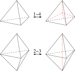
Figure 5: The 1-4 move takes a tetrahedron and subdivides it into four tetrahedra by introducing a new vertex in the center. The 2-3 move take two tetrahedra sharing a face, removes the shared face, and slices the resulting octahedron longitudinally into three tetrahedra.

Although conceptually and mathematically useful, Pachner’s theorem does not directly yield an algorithm for the problem of deciding equivalence of triangulated manifolds. One can search for a sequence of Pachner moves connecting a pair of triangulations, but one does not know when to give up the search, because no upper bound is known on the number of necessary moves. Eventually it was proven that the equivalence problem for 3-manifolds is algorithmically decidable (see [21]), but the problem is not known to be in P. The equivalence problem for $n$-manifolds for any $n\geq 4$ is undecidable[31]. The equivalence problem for orientable 2-manifolds is in P (see appendix A). Lacking an efficient way to decide equivalence of three-manifolds it is natural to look for partial solutions such as those provided by 3-manifold invariants.

In the Ponzano-Regge model, we are given a triangulated 3-manifold. We then associate one $j$-variable to each edge of each tetrahedron. These $j$-variables represent spins and take integer and half-integer values. To a closed manifold the Ponzano-Regge model associates the following amplitude[9].

$$Z_{\mathrm{closed}}=\sum_{j-\mathrm{labelings}}\prod_{\mathrm{edges}}(-1)^{2j}(2j+1)\prod_{\mathrm{faces}}(-1)^{j_{1}+j_{2}+j_{3}}\prod_{\mathrm{tetrahedra}}\left\{\begin{array}[]{ccc}j_{1}&j_{2}&j_{3}\\ j_{4}&j_{5}&j_{6}\end{array}\right\}$$ (18)

The value of the $6j$-symbol is not invariant under the $6!$ permutations of the indices. To get the correct Ponzano-Regge amplitude we must associate the indices in the $6j$ symbol to the edges of a tetrahedron as follows.

(19)

The $6j$ symbol is invariant under the 24 symmetries of a tetrahedron, which shows that this procedure is consistent. The diagram above just indicates that each pair of indices sharing a column in the $6j$ symbol must correspond to a pair of nonadjacent (i.e. opposite) edges in the tetrahedron.

In principle, there are infinitely many $j$-labelings to sum over in equation 18. However, the $6j$-symbol is only nonzero if the triple of $j$-values associated to each face is admissible by the rules of quantum angular momentum addition, described in equation 11. Thus, in some cases, the Ponzano-Regge amplitude contains only finitely many nonzero terms. In the case of infinitely many admissible labelings, the sum often diverges. We return to the question of which triangulations yield finite amplitudes below, but first we describe the Ponzano-Regge amplitude associated to a 3-manifold with boundary.

Let $M$ be a 3-manifold whose boundary is the union of the 2-manifolds $A$ and $B$. That is, $M$ is a generalized cobordism between $A$ and $B$. The triangulation (by tetrahedra) of $M$ induces triangulations (by triangles) of $A$ and $B$. Each edge of a triangulation of $M$ is either internal, on the boundary $A$, on the boundary $B$, or on both $A$ and $B$. The same applies to the faces. To any labeling of the boundaries, the Ponzano-Regge model associates the following amplitude, where the sum is over $j$-labelings of internal edges.

$$Z = \sum_{j-\mathrm{labelings}}\left(\prod_{e\in\mathrm{edges}}\left[(-1)^{2j_{e}}(2j_{e}+1)\right]^{(2-b(e))/2}\times\right.$$

$$\left.\prod_{f\in\mathrm{faces}}\left[(-1)^{j_{f(1)}+j_{f(2)}+j_{f(3)}}\right]^{(2-b(f))/2}\prod_{t\in\mathrm{tetrahedra}}\left\{\begin{array}[]{ccc}j_{t(1)}&j_{t(2)}&j_{t(3)}\\ j_{t(4)}&j_{t(5)}&j_{t(6)}\end{array}\right\}\right)$$

Here $b(e)$ is the number of boundaries on which the edge $e$ lies, 0, 1, or 2. Similarly, $b(f)\in\{0,1,2\}$ is the number of boundaries on which the face $f$ lies. $\{f(1),f(2),f(3)\}$ are the three edges of face $f$, and $\{t(1),t(2),t(3),t(4),t(5),t(6)\}$ are the six edges of tetrahedron $t$. We recover equation 18 as the special case when all edges and faces are internal ($b(e)=0\ \forall e$ and $b(f)=0\ \forall f$).

To each boundary we can associate a (possibly infinite-dimensional) Hilbert space corresponding to all admissible labelings of the triangulation. The Ponzano-Regge amplitudes between a pair of labelings is thus a matrix element of a linear transformation between these Hilbert spaces. This mapping from cobordisms to linear transformations obeys the functoriality property 17. That is, when we compose two cobordisms, we compose the corresponding linear transformations. To see this, note that by the usual rule of matrix multiplication, we sum over the labelings of the edges that we have glued. This is consistent with the prescription for calculating the Ponzano-Regge amplitude for the resulting single cobordism because these edges have now become internal. Furthermore, each edge $e$ has one factor of $\sqrt{(-1)^{2j_{e}}(2j_{e}+1)}$ from each of the two matrices we have multiplied, resulting in a factor of $(-1)^{2j_{e}}(2j_{e}+1)$, as befits an internal edge. Similarly, the faces that are glued pick up one factor of $\sqrt{(-1)^{j_{f(1)}+j_{f(2)}+j_{f(3)}}}$ from each of the linear transformations being composed, giving them the correct weighting for an internal face.

For a three-dimensional quantum field theory on triangulated manifolds to be topological, it should be independent of triangulation, that is, invariant under the Pachner moves. The Ponzano-Regge model fails to be topological in general. It is invariant under the 2-3 Pachner move as a consequence of the Beidenharn-Elliot identity for $6j$ symbols[47]:

$$\sum_{x}(-1)^{\phi}(2x+1)\left\{\begin{array}[]{ccc}a&b&x\\ c&d&g\end{array}\right\}\left\{\begin{array}[]{ccc}c&d&x\\ e&f&h\end{array}\right\}\left\{\begin{array}[]{ccc}e&f&x\\ b&a&j\end{array}\right\}=\left\{\begin{array}[]{ccc}j&h&j\\ e&a&d\end{array}\right\}\left\{\begin{array}[]{ccc}g&h&j\\ f&b&c\end{array}\right\},$$

where $\phi=a+b+c+d+e+f+g+h+x+j$. However, it is not invariant under the 1-4 move. In fact, by applying the 1-4 move one can go from a triangulation whose Ponzano-Regge amplitude has finitely many terms to one whose amplitude has infinitely many terms. A Ponzano-Regge amplitude with infinitely many terms could still be convergent, but generically this seems not to be the case[9].

In a Ponzano-Regge summation for a 3-manifold with boundary, the boundary conditions (i.e. the $j$-labels on the boundary edges) limit the admissible labels on the internal edges. For some triangulations this limitation ensures that there are only finitely many possible labels on every edge. For other triangulations there exist some internal edges whose label is not constrained to a finite set by the boundary conditions. Barrett and Naish-Guzman call the set of edges whose labels are not constrained to a finite set the “tardis” of the triangulation. The tardis depends only on the manifold and its triangulation, not on the particular $j$-values assigned to the boundary. The Ponzano-Regge amplitudes between boundary labellings of a triangulation whose tardis is the empty set (called a non-tardis triangulation in [9]) are finite. Furthermore, as proven in [9],

Theorem 2

[9] Let $M$ be a manifold with a fixed triangulation of its boundary. Then any two non-tardis triangulations compatible with the given boundary triangulation yield the same Ponzano-Regge amplitudes.

For the class of non-tardis triangulations the Ponzano-Regge model thus acts as a topological quantum field theory. It is also worth noting that given a triangulation with $n$ tetrahedra, a classical computer can decide whether it is non-tardis in $\mathrm{poly}(n)$ time[9].

6 Approximating Ponzano-Regge Transition Amplitudes

In this section we show that for a certain subclass of non-tardis triangulations the Ponzano-Regge transition amplitudes can be efficiently approximated to polynomial additive precision on a permutational quantum computer.

A single tetrahedron is a triangulation of the 3-ball. Its boundary is a triangulated 2-sphere. We can divide the 2-sphere boundary into a pair of discs, and think of the 3-ball as a generalized cobordism between these two discs. We can do this such that each disc is triangulated into two triangles, as shown below.

(21)

The six lines in diagram 21 are the edges of a tetrahedron. The vertical line lies in the top disc, the horizontal line lies in the bottom disc, and the thick lines around the perimeter lie on both discs. The Ponzano-Regge model associates an infinite-dimensional Hilbert space to the two-face triangulation of a disc, namely the formal span of all admissible labelings of the five edges of the triangulation. Corresponding to the tetrahedron we have a linear transformation $M_{\mathrm{tet}}:\includegraphics[width=15.00002pt]{hdiamond.eps}\to\includegraphics[width=15.00002pt]{hdiamond.eps}$. $M_{\mathrm{tet}}$ is completely specified by the matrix elements between each pair of admissible labellings of the disc triangulations. By the definitions given in the previous section, these matrix elements are

$$\left<\begin{array}[]{c}\includegraphics[width=28.45274pt]{bottom.eps}\end{array}\right|M_{\mathrm{tet}}\left|\begin{array}[]{c}\includegraphics[width=28.45274pt]{top.eps}\end{array}\right> = \sqrt{(-1)^{2f}(2f+1)}\sqrt{(-1)^{2d}(2d+1)}\times$$ (27)

$$\sqrt{(-1)^{c+b+d}}\sqrt{(-1)^{d+e+a}}\sqrt{(-1)^{c+e+f}}\sqrt{(-1)^{b+a+f}}\left\{\begin{array}[]{ccc}a&b&f\\ c&e&d\end{array}\right\}$$

Simplifying this expression, we recognize it as

$$\left[\begin{array}[]{ccc}a&b&f\\ c&e&d\end{array}\right],$$ (28)

the recoupling tensor from equation 6. This observation generalizes as follows.

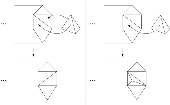
Figure 6: On the left we glue two adjacent faces of a tetrahedron to two adjacent triangles of the boundary of a 3-manifold. The result is a new triangulation of the boundary in which one edge has been flipped. On the right we instead glue only one face of the tetrahedron. In the resulting triangulation one of the triangles gets split into three.

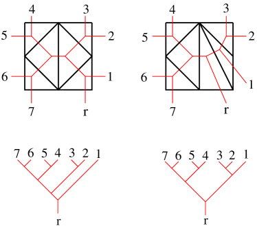
Figure 7: Flipping an edge of a triangulation induces a change on the corresponding dual triangulation. If the dual triangulation is a tree, then this corresponds to a recoupling of spins. Here we have chosen one edge as the root and labeled it “r”. We then draw the dual tree in more conventional shape to illustrate the connection to recoupling moves discussed in section 2. We have added arbitrary labels to the other leaves for clarity.

We can build up a 3-manifold by gluing on additional tetrahedra one by one. As we do so, the triangulation of the surface gets modified. The change in triangulation depends on how many faces of the new tetrahedron we glue to existing faces, as illustrated in figure 6. Thus the gluing of a tetrahedron can be thought of as a cobordism or as a retriangulation of the boundary of a three-manifold. In particular if we glue two faces of a tetrahedron we correspondingly flip one edge of the triangulation.

The dual to a $j$-labeled triangulation is another $j$-labeled graph, as illustrated in figure 7. If this $j$-labeled dual graph is a tree, then the flip move on the original graph translates to a recoupling move on the dual tree. (See figure 7.) The linear transformation that the Ponzano-Regge model associates to this cobordism is identical to the recoupling transformation of the corresponding $j$-labeled dual tree.

In the permutational model we can efficiently find a polynomial additive approximation to the matrix elements between any pair of $j$-labeled binary trees in time polynomial in the number of leaves. Thus, the following problem can be solved on a permutational quantum computer in $\mathrm{poly}(n,m,1/\epsilon)$ time.

Problem 2: Approximate Ponzano-Regge transition amplitude. Input: We are given two triangulated surfaces $A$ and $B$ such that the dual to the triangulations are both binary trees of $n$ leaves. We are also given sequence of $m$ pairs of neighboring triangles on which to glue two faces of successive tetrahedra. This induces a sequence of edge flips taking us from triangulation $A$ to triangulation $B$. We are given $j$-labelings for $A$ and $B$. Lastly, we are given positive parameter $\epsilon$. Output: The real and imaginary parts of Ponzano-Regge transition amplitude corresponding to the above cobordism, to within $\pm\epsilon$.

Note that the class of cobordisms described in problem 2 is quite restricted. In general triangulated surfaces may not have duals that are binary trees. Furthermore, as illustrated in figure 6, there are ways to glue tetrahedra onto a surface other than two faces at a time. It is an open problem whether permutational quantum computers can efficiently approximate Ponzano-Regge transition amplitudes for a more general class of cobordisms. On the other hand, it is clear that problem 2 is a complete problem for the “pure recoupling” class of permutational quantum computations, in which the binary trees are chosen arbitrarily, but the permutation is fixed to be the identity.

7 Mixed States

In this section we consider a modified version of permutational quantum computation in which the initial state is highly mixed. We then show that the resulting complexity class is contained in BPP. In contrast, if we take the standard quantum circuit model and analogously apply it to highly mixed initial states, we obtain a complexity class DQC1 which appears to extend beyond BPP, although it is probably weaker than BQP. We start by describing DQC1.

In the standard quantum circuit model, one begins with a canonical pure state, such as $\left|{0}\right\rangle^{\otimes n}$, applies a quantum circuit, and then performs a simple measurement, such as measuring each qubit independently in the $\{\left|{0}\right\rangle,\left|{1}\right\rangle\}$ basis. Experimentally, it is often difficult to obtain the initial pure state $\left|{0}\right\rangle^{\otimes n}$. In particular, several of the early quantum computing experiments used liquid state NMR, in which the quantum states being manipulated are highly mixed. This led to some debate as to whether the NMR experiments were truly quantum computation.

To address this issue, Knill and Laflamme introduced an idealized model of quantum computation on highly mixed states, called the one clean qubit model[29]. In this model one is given the initial state $\rho$ in which one qubit is in a pure state and the remaining $n$ qubits are maximally mixed.

$$\rho=\left|{0}\right\rangle\left\langle{0}\right|\otimes\frac{I}{2^{n}}$$

Then one is allowed to apply polynomially many quantum gates to this state, and lastly measure the first qubit in the $\{\left|{0}\right\rangle,\left|{1}\right\rangle\}$ basis. The complexity class of problems solvable in polynomial time in this model is called DQC1.

Let $C$ be a quantum circuit on $n$ qubits and let $U_{C}$ be the corresponding $2^{n}\times 2^{n}$ unitary matrix. The problem of estimating $\mathrm{Tr}(U_{C})$ is DQC1-complete[29, 45]. A certain problem of estimating Jones polynomials is also DQC1-complete[46], and the generalization to HOMFLY polynomials is also efficiently solvable on one clean qubit computers[26]. No polynomial time algorithms for these problems are known. On the other hand, most evidence suggests that one clean qubit computers are less powerful than standard quantum computers[5, 14]. Just as with PQP, one must be careful in choosing what sort of computer controls the experiments performed on the qubits. If this computer is a P machine then DQC1 automatically contains P. To make a more meaningful comparison to classical computation it is better to choose a weaker computational model such as L or NC1 to control the experiments (see [1] for the definitions of these complexity classes). The conjectured relationships between P, BQP, and DQC1 are illustrated in figure 8.

Figure 8: This diagram shows the conjectured relationships between classical polynomial time (P), quantum polynomial time (BQP), and one clean qubit (DQC1). P and DQC1 are known rigorously to be contained in BQP but the containments are not known rigorously to be strict.

The one clean qubit model is not necessarily physically realistic in its details. Nevertheless, it provides a proof of principle that quantum computation on highly mixed states is still probably capable of achieving exponential speedups over classical computers for certain problems. Furthermore, it provides perhaps the only model of quantum computation other than PQP which yields a complexity class apparently distinct from BQP but not contained in P.

We can similarly formulate a one clean qubit version of the permutational model. By analogy to DQC1 we define the one clean qubit version of PQP to be the set of problems efficiently solvable given the ability to approximate the trace of irreducible representations of $S_{n}$ (i.e. characters) to $\pm\epsilon$ precision in $\mathrm{poly}(n,1/\epsilon)$ time. Such a definition seems mathematically natural. Furthermore, it is equivalent to a somewhat natural physical model, as follows. We start with the initial state

$$\rho_{J}=\left|{\psi}\right\rangle\left\langle{\psi}\right|\otimes\frac{1}{d_{J}}\sum_{x=1}^{d_{J}}\left|{J,x}\right\rangle\left\langle{J,x}\right|$$

on $n+1$ spin-1/2 particles. Here $\left|{\psi}\right\rangle=\alpha\left|{0}\right\rangle+\beta\left|{1}\right\rangle$ is an arbitrary pure state on one spin, and $\left|{J,1}\right\rangle,\left|{J,2}\right\rangle,\ldots,\left|{J,d_{J}}\right\rangle$ is a complete basis for the space of states of $n$ spins with total angular momentum $J$. Thus these $n$ spins are in the maximally mixed state within the subspace of total angular momentum $J$. We then perform a coherently controlled permutation on the $n$ maximally mixed spins, and measure the back-action on the first spin, as illustrated below.

This type of interferometric measurement is standard in quantum computing and is known as the Hadamard test. The final measurement is in the $\{\left|{0}\right\rangle,\left|{1}\right\rangle\}$ basis. The probability of outcome $\left|{0}\right\rangle$ is

$$p_{0}=\frac{1}{2}\left[1+2\mathrm{Re}\left(\frac{\alpha^{*}\beta\sum_{x=1}^{d_{J}}\left\langle{J,x}\right|U_{\pi}\left|{J,x}\right\rangle}{d_{J}}\right)\right].$$

As discussed in section 2, $U_{\pi}$ acts on the span of $\left|{J,1}\right\rangle,\left|{J,2}\right\rangle,\ldots,\left|{J,d_{J}}\right\rangle$ as an irreducible representation of $S_{n}$. Specifically, $U_{\pi}$ acts as the irreducible representation corresponding to a Young diagram of two rows where the overhang of the top row over the bottom row is $2J$. Thus,

$$p_{0}=\frac{1}{2}\left[1+2\mathrm{Re}\left(\alpha^{*}\beta\frac{\chi_{J}}{d_{J}}\right)\right],$$

where $\chi_{J}$ is the character of this irreducible representation.

By performing the Hadamard test $O(1/\epsilon^{2})$ times with $\alpha=\beta=\frac{1}{\sqrt{2}}$ one can estimate $\mathrm{Re}\left(\frac{\chi_{J}}{d_{J}}\right)$ to within $\pm\epsilon$. Similarly, choosing $\alpha=\frac{1}{\sqrt{2}}$, $\beta=-\frac{i}{\sqrt{2}}$ yields $\mathrm{Im}\left(\frac{\chi_{J}}{d_{J}}\right)$. Thus this model efficiently solves the problem of estimating $\frac{\chi_{J}}{d_{J}}$ to polynomial additive precision. Furthermore, simulating this model reduces to the problem of estimating $\frac{\chi_{J}}{d_{J}}$ to polynomial additive precision. Thus this problem is complete for the one clean qubit version of permutational quantum computation. Note that the hardness result holds for any choice of projective measurement, not just $\begin{array}[]{c}\mbox{\lx@xy@svg{\hbox{\raise 0.0pt\hbox{\kern 0.0pt\hbox{\ignorespaces\ignorespaces\ignorespaces\hbox{\vtop{\kern 0.0pt\offinterlineskip\halign{\entry@#!@&&\entry@@#!@\cr&&\crcr}}}\ignorespaces{\hbox{\kern 0.0pt\raise 0.0pt\hbox{\hbox{\kern-3.0pt\raise 0.0pt\hbox{\hbox{\kern 3.0pt\raise 0.0pt\hbox{$\textstyle{}$}}}}}}}{\hbox{\kern 8.00003pt\raise 0.0pt\hbox{\hbox{\kern 0.0pt\raise 0.0pt\hbox{$\textstyle{\lx@xy@svgnested{\hbox{\raise 0.0pt\hbox{\kern 7.56252pt\hbox{{\hbox{\kern-7.56252pt\raise 0.0pt\hbox{\hbox{\kern 3.00003pt\raise-3.41666pt\hbox{$\textstyle{H}$}}}}}\ignorespaces\ignorespaces\ignorespaces\ignorespaces\ignorespaces{\hbox{\lx@xy@droprule}}\ignorespaces\ignorespaces\ignorespaces\ignorespaces\ignorespaces\ignorespaces{\hbox{\lx@xy@droprule}}\ignorespaces\ignorespaces\ignorespaces\ignorespaces\ignorespaces\ignorespaces{\hbox{\lx@xy@droprule}}\ignorespaces\ignorespaces\ignorespaces\ignorespaces\ignorespaces{\hbox{\lx@xy@droprule}}}}}}}$}}}}}\ignorespaces\ignorespaces\ignorespaces\ignorespaces{}{\hbox{\lx@xy@droprule}}\ignorespaces{}{\hbox{\lx@xy@droprule}}{\hbox{\lx@xy@droprule}}{\hbox{\kern 31.12509pt\raise 0.0pt\hbox{\hbox{\kern 0.0pt\raise 0.0pt\hbox{$\textstyle{\lx@xy@svgnested{\hbox{\raise 0.0pt\hbox{\kern 9.00009pt\hbox{{\hbox{\kern-9.00009pt\raise 0.0pt\hbox{\hbox{\kern 3.00003pt\raise 0.0pt\hbox{$\textstyle{\lx@xy@svgnested{\hbox{\raise 0.0pt\hbox{\kern 6.00006pt\hbox{{\hbox{\kern-11.00008pt\raise 0.0pt\hbox{\hbox{\kern 0.0pt\raise-11.00008pt\hbox{\cirbuild@}}}}}\ignorespaces\ignorespaces\ignorespaces\ignorespaces{\hbox{\lx@xy@drawline@}}{}{}}}}}}$}}}}}\ignorespaces\ignorespaces\ignorespaces\ignorespaces\ignorespaces{\hbox{\lx@xy@droprule}}\ignorespaces\ignorespaces\ignorespaces\ignorespaces\ignorespaces\ignorespaces{\hbox{\lx@xy@droprule}}\ignorespaces\ignorespaces\ignorespaces\ignorespaces\ignorespaces\ignorespaces{\hbox{\lx@xy@droprule}}\ignorespaces\ignorespaces\ignorespaces\ignorespaces\ignorespaces{\hbox{\lx@xy@droprule}}}}}}}$}}}}}\ignorespaces\ignorespaces\ignorespaces\ignorespaces{}{\hbox{\lx@xy@droprule}}\ignorespaces{}{\hbox{\lx@xy@droprule}}{\hbox{\lx@xy@droprule}}\ignorespaces}}}}\ignorespaces}\end{array}$.

As shown in [23], the normalized character of any irreducible representation of the symmetric group can be approximated to $\pm\epsilon$ with probability $1-\delta$ in $\mathrm{poly}(n,1/\epsilon,\log(1/\delta))$ time on a classical computer using an algorithm based on random sampling. This shows that the one clean qubit version of PQP is contained in the complexity class BPP. This contrasts with DQC1, which is unlikely to be contained in BPP. One could interpret this as a form of indirect evidence that PQP is weaker than BQP.

An arguably more compelling comparison can be made to topological computation. The problem of estimating a particular matrix element of the Fibonacci representation of the braid group $B_{n}$ is BQP-complete[19, 3, 2]. Estimating the characters of the Fibonacci representation is DQC1-complete[46]. The Fibonacci representation of the braid group is closely related to Young’s orthogonal representation of the symmetric group. More precisely, as discussed in [28], the former is a $q$-deformation of the latter. The fact that estimating characters of $S_{n}$ is easier than estimating the characters of the corresponding Fibonacci representation of $B_{n}$ suggests that estimating matrix elements of Young’s orthogonal form may be easier than estimating matrix elements of the Fibonacci representation. That is, it suggests that estimating matrix elements of Young’s orthogonal form may not be BQP-complete.

8 Fault Tolerance

To implement a permutational quantum computation, one prepares spins into states of known total angular momentum, moves the spins around, and measures total angular momentum. For a fixed number of spins, the set of allowed operations is discrete and finite. Errors in the trajectories of the spins do not cause computational errors unless the trajectory is so deformed as to implement a different permutation than that intended. In this respect, the permutational model is similar to the topological model. In the topological model, trajectory errors do not cause computational errors unless they are large enough to induce a braid other than the one intended.

There is a second, more subtle way in which permutational quantum computers are resistant to error; they are impervious to the effects of uniform magnetic fields. A uniform magnetic field $\vec{B}$ acts on $n$ spin-1/2 particles through the Hamiltonian

$$H_{\vec{B}}=\vec{B}\cdot\sum_{i=1}^{n}\vec{S}_{i},$$

where $\vec{S}_{i}$ is the angular momentum operator on spin $i$, as described in equation 1. Applying this Hamiltonian for time $t$ induces the unitary transformation

$$U_{\vec{B}}(t)=e^{-iH_{\vec{B}}t}=u^{\otimes n}$$

for some $u\in SU(2)$.

The unitary transformation $u^{\otimes n}$ commutes with the total angular momentum operator $S_{b}$ for any subset $b$ of the $n$ spin-1/2 particles. Thus, it does not affect the computation. Recall from section 2 that in addition to total angular momenta of various subsets of spins, we need the operator

$$Z_{\mathrm{total}}=\frac{1}{2}\sum_{i=1}^{n}\sigma_{z}^{(i)}$$

to obtain a complete set of commuting observables. $u^{\otimes n}$ affects only the degree of freedom described by the eigenvalue of this operator. (This is an example of Schur-Weyl duality[7].) In the language of quantum error correction, the space of $j$-labeled tree states is a noiseless subsystem[30] with respect to errors of the form $u^{\otimes n}$.

9 Concluding Remarks

In this paper we analyze a model of quantum computation based on the permutation of spin-1/2 particles. We call the set of problems solvable in this model in polynomial time PQP. Permutational computers can be simulated efficiently by standard quantum computers. Thus PQP is contained in BQP. On the other hand, we have presented two quantum algorithms for permutational quantum computers that seem to exhibit exponential speedup over classical computation. Thus it seems unlikely that PQP is contained in P.

The question of whether PQP is equal to BQP remains open. In other words, we do not know whether permutational quantum computers are universal. To begin to address this question, we first review the techniques that were used to prove the universality of the quantum circuits and topological quantum computers.

In principle, the set of unitary transformations that one might wish to perform on $n$ qubits is a compact but continuous group $SU(2^{n})$. In contrast, the set of quantum circuits achievable with a finite gate set is discrete. Nevertheless, certain finite sets of gates achieve universality in the sense that the discrete infinite set of unitaries achievable by composing these gates into quantum circuits is dense in $SU(2^{n})$ [35]. Thus any desired unitary in $SU(2^{n})$ can be approximated to any desired level of precision by a sufficiently large quantum circuit. To approximate an arbitrary unitary on $n$ qubits to $1/\mathrm{poly}(n)$ precision requires exponentially many gates in general. Most research on quantum computation focuses on the small subset of $SU(2^{n})$ implementable by circuits of $\mathrm{poly}(n)$ gates. Using the Solovay-Kitaev theorem[35], one can show that this subset does not depend on the choice of gate set. That is, any universal gate set can simulate any other with only logarithmic overhead.

Similarly, the braid group $B_{m}$ on $m$ strands is a discrete infinite group for any fixed $m$. As shown in [19, 18, 3, 2], the unitary representations of $B_{m}$ induced by certain anyons are dense in the corresponding unitary groups. Furthermore, these authors show that the set of unitaries approximable by braids of polynomially many crossings coincides with the set of unitaries approximable by quantum circuits of polynomially many gates.

The permutational model of quantum computation is very different from the quantum circuit model and anyonic models in that the set of unitaries achievable with $n$ spins is finite. As discussed in [32], the number coupling schemes for $n$ spins, which we represent as binary trees of $n$ leaves, is $C_{n-1}$, where $C_{n}$ is the $n^{\mathrm{th}}$ Catalan number

$$C_{n}=\frac{(2n)!}{(n+1)!n!}.$$

When specifying a permutational computation we choose two such couplings and one of the $n!$ possible permutations. Thus, the number of implementable unitary transformations is upper bounded by $n!C_{n-1}^{2}$. By Stirling’s approximation this is $2^{O(n\log n)}$. In contrast, suppose we want to choose a finite subset $S$ of $SU(d)$ such that for any $u\in SU(d)$ there exists $v\in S$ such that $\|v-u\|<\epsilon$. As discussed in [24], for fixed $\epsilon$ the smallest set $S$ satisfying this density condition has exponentially many elements as a function of $d$. The unitary transformations of an $n$-spin permutational computer act on a Hilbert space whose dimension is exponential in $n$. Any dense subset of the unitaries on this Hilbert space would therefore have a doubly exponential number of elements. Thus the set of $2^{O(n\log n)}$ unitaries actually implementable on a permutational quantum computer is very far from dense.

The limited number of unitaries implementable by a permutational quantum computer with a fixed number of spins means that the standard universality arguments based on density cannot work. If permutational computers are universal their method of simulating quantum circuits will have to use a number of spins that scales not only with the number of qubits on which the quantum circuit acts, but also on the number of gates in the circuit. Arguably the failure of standard techniques of proving universality and the fact that the one clean qubit version of permutational quantum computation is weaker than the one clean qubit version of standard quantum computation suggest that PQP is in fact weaker than BQP.

The problem of whether PQP even contains all of P is also an open question. It could be that PQP and P are incomparable, that is, classical computers and permutational quantum computers can each solve some problems in polynomial time that the other cannot. Note that, as discussed in section 2, analysis of this question requires a careful formulation of PQP.

The physical implementation of permutational quantum computers raises many additional questions. For one, the problem of finding a physically realistic method to implement the interferometric measurements discussed in section 2 remains unsolved. Without these we obtain a slightly weaker version of permutational quantum computation in which the phase information is unrecoverable.

In addition, one could investigate potential implementations of the permutational model other than the actual manipulation of spin-1/2 particles. One possibility is to find a material whose quasiparticles obey the “braiding” and recoupling rules described in 4 and 5. In other words, one could attempt to implement permutational quantum computation as a special case of anyonic computation. As a more exotic possibility, it has been proposed that in addition to Fermions and Bosons, which exchange according to the two one-dimensional representations of the symmetric group, there could also exist fundamental particles that exchange according to higher dimensional representations of the symmetric group. Such particles are said to obey parastatistics[40]. Fundamental particles obeying parastatistics have never been observed, but if they were, they would provide a computational resource akin to permutational quantum computing.

Finding more algorithms for permutational quantum computers provides another direction for further research. In particular, it does not seem obvious that the class of Ponzano-Regge transition amplitudes approximated by the algorithm of section 6 exhausts the capabilities of permutational quantum computers. It would be interesting to attempt to fully characterize the set of Ponzano-Regge spin foams efficiently approximable in PQP.

10 Acknowledgements

In doing the work reported in this paper, I have benefitted from conversations with numerous people. I especially thank Laurent Freidel, Gorjan Alagic, and Liang Kong. I gratefully acknowledge support from the Sherman Fairchild foundation and the National Science Foundation under grant PHY-0803371, as well as the hospitality of the Perimeter Institute.

Appendix A Algorithm for two-manifold Equivalence

Closed orientable two-manifolds are completely specified up to homeomorphism by a single integer, the genus, which counts how many “handles” a surface has, as illustrated below.

Genus is thus a complete two-manifold invariant; computing it solves the 2-manifold equivalence problem. Euler showed that any closed triangulated orientable 2-manifold satisfies the formula

$$V-E+F=2-2g,$$

where $V$ is the number of vertices, $E$ the number of edges, and $F$ the number of faces in the triangulation, and $g$ is the genus. Thus, $g$ can be computed in time polynomial in the size of the triangulation.

Appendix B Ponzano-Regge model as Quantum Gravity

According to general relativity, spacetime is a manifold that locally looks Minkowskian. That is, within a sufficiently small region of spacetime there exists a choice of basis such that the distance metric is

$$\left[\begin{array}[]{cccc}-1&0&0&0\\ 0&1&0&0\\ 0&0&1&0\\ 0&0&0&1\end{array}\right].$$

The vector component corresponding to the $-1$ matrix element is time, and the three remaining components are space. Such a spacetime is often referred to as $(3+1)$-dimensional to indicate the three spatial dimensions and single time dimension.

One can formulate $(n+m)$-dimensional analogues of general relativity for any integers $n$ and $m$. In particular, the $(3+0)$-dimensional analogue of general relativity, which uses the ordinary Riemannian metric

$$\left[\begin{array}[]{ccc}1&0&0\\ 0&1&0\\ 0&0&1\end{array}\right]$$

turns out to be topological[8]. Due to the difficulty of formulating physically realistic quantum gravity, some physicists have chosen to investigate quantum versions of $(3+0)$-dimensional gravity. Due to its topological nature and other mathematical conveniences, this seems to be easier than the full $(3+1)$-dimensional case. Thus $(3+0)$-dimensional quantum gravity may serve as a useful toy model on which to develop intuitions and techniques needed to approach the full $(3+1)$-dimensional case.

The Ponzano-Regge model[41] is one proposed model of $(3+0)$-dimensional quantum gravity. It is an example of a spin foam model. The spin foam models are closely inspired by, but distinct from, loop quantum gravity theories, which are obtained by applying canonical quantization methods to general relativity. Interestingly, a completely different motivation for the use of spin-networks in describing gravity, not related to canonical quantization, was earlier given by Penrose[39].

References

- [1] Scott Aaronson and Greg Kuperburg. The complexity zoo. qwiki.stanford.edu/wiki/Complexity_Zoo.
- [2] Dorit Aharonov and Itai Arad. The BQP-hardness of approximating the Jones polynomial. arXiv:quant-ph/0605181, 2006.
- [3] Dorit Aharonov, Vaughan Jones, and Zeph Landau. A polynomial quantum algorithm for approximating the Jones polynomial. In Proceedings of the 38th ACM Symposium on Theory of Computing, 2006. arXiv:quant-ph/0511096.
- [4] Dorit Aharonov, Wim van Dam, Julia Kempe, Zeph Landau, Seth Lloyd, and Oded Regev. Adiabatic quantum computation is equivalent to standard quantum computation. SIAM Journal of Computing, 37(1):166–194, 2007. arXiv:quant-ph/0405098.
- [5] Andris Ambainis, Leonard Schulman, and Umesh Vazirani. Computing with highly mixed states. Journal of the ACM, 53(3):507–531, May 2006. arXiv:quant-ph/0003136.
- [6] Michael Atiyah. Topological quantum field theories. Publications Mathématiques de l’I.H.É.S., 68:175–186, 1988.
- [7] Dave Bacon, Isaac L. Chuang, and Aram W. Harrow. The quantum Schur transform: I. efficient qudit circuits. In Proceedings of the eighteenth annual ACM-SIAM symposium on Discrete algorithms (SODA), pages 1235–1244, 2007. arXiv:quant-ph/0601001.
- [8] John C. Baez. An introduction to spin foam models of BF theory and quantum gravity. In Helmut Gausterer and Harald Grosse, editors, Geometry and Quantum Physics, pages 25–93. Springer, 2001. arXiv:gr-qc/9905087.
- [9] John W. Barrett and Ileana Naish-Guzman. The Ponzano-Regge model. arXiv:0803.3319, 2008.
- [10] H. Boerner. Representations of Groups. North-Holland, 1963.
- [11] Andrew M. Childs. Universal computation by quantum walk. arXiv:0806.1972, 2008.
- [12] R. Cleve, A. Ekert, C. Macchiavello, and M. Mosca. Quantum algorithms revisited. Proceedings of the Royal Society of London, Series A, 454(1969):339–354, 1998. arXiv:quant-ph/9708016.
- [13] Joseph M. Clifton. A simplification of the computation of the natural representation of the symmetric group . Proceedings of the American Mathematical Society, 83(2):248–250, 1981.
- [14] Animesh Datta, Steven T. Flammia, and Carlton M. Caves. Entanglement and the power of one qubit. Physical Review A, 72(042316), 2005. arXiv:quant-ph/0505213.
- [15] G. de B. Robinson, editor. The collected papers of Alfred Young 1873-1940. Number 21 in Mathematical Expositions. University of Toronto Press, 1977.
- [16] David Deutsch. Quantum computational networks. Proceedings of the Royal Society of London A, 425:73–90, 1989.
- [17] Edward Farhi, Jeffrey Goldstone, and Sam Gutmann. A quantum algorithm for the Hamiltonian NAND tree. Theory of Computing, 4:169–190, 2008. arXiv:quant-ph/0702144.
- [18] Michael Freedman, Alexei Kitaev, and Zhenghan Wang. Simulation of topological field theories by quantum computers. Communications in Mathematical Physics, 227:587–603, 2002.
- [19] Michael Freedman, Michael Larsen, and Zhenghan Wang. A modular functor which is universal for quantum computation. Communications in Mathematical Physics, 227(3):605–622, 2002. arXiv:quant-ph/0001108.
- [20] S. Gelfand and D. Kazhdan. Invariants of three-dimensional manifolds. Geometric and Functional Analysis, 6(2):268–300, 1996.
- [21] Timothy Gowers, June Barrow-Green, and Imre Leader, editors. The Princeton Companion to Mathematics, chapter IV.10, page 440. Princeton University Press, 2008.
- [22] Morton Hamermesh. Group Theory and its Application to Physical Problems. Addison-Wesley, 1962.
- [23] Stephen P. Jordan. Fast quantum algorithms for approximating some irreducible representations of groups. arXiv:0811.0562, 2008.
- [24] Stephen P. Jordan. Quantum Computation Beyond the Circuit Model. PhD thesis, Massachusetts Institute of Technology, 2008. arXiv:0809.2307.
- [25] Stephen P. Jordan and Pawel Wocjan. Efficient quantum circuits for arbitrary sparse unitaries. arXiv:0904.2211, 2009.
- [26] Stephen P. Jordan and Pawel Wocjan. Estimating Jones and HOMFLY polynomials with one clean qubit. Quantum Information and Computation, 9(3/4):264–289, 2009. arXiv:0807.4688.
- [27] William M. Kaminsky, Seth Lloyd, and Terry P. Orlando. Scalable superconducting architecture for adiabatic quantum computation. arXiv:quant-ph/0403090, 2004.
- [28] Louis H. Kauffman and Samuel J. Lomonaco Jr. q-deformed spin networks, knot polynomials, and anyonic topological quantum computation. Journal of Knot Theory, 16(3):267–332, 2007. arXiv:quant-ph/0606114.
- [29] E. Knill and R. Laflamme. Power of one bit of quantum information. Physical Review Letters, 81(25):5672–5675, 1998. arXiv:quant-ph/9802037.
- [30] Daniel A. Lidar and K. Birgitta Whaley. Irreversible Quantum Dynamics, volume 622 of Lecture Notes in Physics, chapter Decoherence-Free Subspaces and Subsystems, pages 83–120. Springer, Berlin, 2003. arXiv:quant-ph/0301032.
- [31] Andrei Andreevich Markov. The unsolvability of the problem of homeomorphism. Dokladi Akademii Nauk SSSR, 121:218–220, 1958. See also [21].
- [32] Annalisa Marzuoli and Mario Rasetti. Computing spin networks. Annals of Physics, 318:345–407, 2005.
- [33] Cristopher Moore, Daniel Rockmore, and Alexander Russell. Generic quantum Fourier transforms. In SODA ’04: Proceedings of the fifteenth annual ACM-SIAM Symposium On Discrete Algorithms, pages 778–787. Society for Industrial and Applied Mathematics, 2004. arXiv:quant-ph/0304064.
- [34] Michael A. Nielsen. Optical quantum computation using cluster states. Physical Review Letters, 93:040503, 2004.
- [35] Michael A. Nielsen and Isaac L. Chuang. Quantum Computation and Quantum Information. Cambridge University Press, Cambridge, UK, 2000.
- [36] Udo Pachner. Über die bistellare äquivalenz simplizialer sphären und polytope. Mathematizche Zeitschrift, 176:565–576, 1981. For reference in English see [20].
- [37] Ruben Pauncz. Alternant molecular orbital method. Studies in Physics and Chemistry. W. B. Saunders Company, 1967. especially see appendix 2.
- [38] Ruben Pauncz. The Symmetric Group in Quantum Chemistry. CRC Press, 1995.
- [39] Roger Penrose. Angular momentum: an approach to combinatorial space-time. In T. Bastin, editor, Quantum Theory and Beyond, pages 151–180. Cambridge University Press, 1971.
- [40] Asher Peres. Quantum Theory: Concepts and Methods. Kluwer, 1993.
- [41] G. Ponzano and T. Regge. Semiclassical limit of Racah coefficients. In F. Bloch, S. G. Cohen, A. de Shalit, S. Sambursky, and I. Talmi, editors, Spectroscopic and group theoretical methods in physics, pages 1–58. North-Holland, 1968.
- [42] Robert Raussendorf and Hans J. Briegel. A one way quantum computer. Physical Review Letters, 86:5188, 2001. arXiv:quant-ph/0010033.
- [43] Sten Rettrup. A recursive formula for Young’s orthogonal representation. Chemical Physics Letters, 47(1):59–60, 1977.
- [44] J. J. Sakurai. Modern Quantum Mechanics. Addison Wesley Longman, Reading, MA, revised edition, 1994.
- [45] Dan Shepherd. Computation with unitaries and one pure qubit. arXiv:quant-ph/0608132, 2006.
- [46] Peter W. Shor and Stephen P. Jordan. Estimating Jones polynomials is a complete problem for one clean qubit. Quantum Information and Computation, 8(8/9):681–714, 2008. arXiv:0807.2831.
- [47] Eric Weisstein. Wigner 6j-symbol. From Mathworld. mathworld.wolfram.com/Wigner6j-Symbol.html.
- [48] Wei Wu and Qianer Zhang. An efficient algorithm for evaluating the standard Young-Yamanouchi orthogonal representation with two-column Young tableaux for symmetric groups. Journal of Physics A: Mathematical and General, 25:3737–3747, 1992.
- [49] Wei Wu and Qianer Zhang. The orthogonal and the natural representation for symmetric groups. International Journal of Quantum Chemistry, 50:55–67, 1994.