Universal non stationary dynamics at the depinning transition

Abstract

We study the non-stationary dynamics of an elastic interface in a disordered medium at the depinning transition. We compute the two-time response and correlation functions, found to be universal and characterized by two independent critical exponents. We find a good agreement between two-loop Functional Renormalization Group calculations and molecular dynamics simulations for the scaling forms, and for the response aging exponent $\theta_{R}$. We also describe a dynamical dimensional crossover, observed at long times in the relaxation of a finite system. Our results are relevant for the non-steady driven dynamics of domain walls in ferromagnetic films and contact lines in wetting.

The universal glassy properties that emerge from the frustrating competition between elasticity and disorder are relevant for many experimental systems, such as interfaces describing magnetic Lemerle et al. (1998); Repain et al. (2004); Metaxas et al. (2007); Kim et al. (2009) and ferroelectric Paruch et al. (2005); Tybell et al. (2002) domain walls, contact lines of fluids Moulinet et al. (2004); contactfrg and fracture Ponson et al. (2006); Alava et al. (2006). Disorder leads to pinning, affecting in a dramatic way their dynamical properties. In particular, when driven by an external force $f$ at zero temperature, disorder leads to a depinning transition at a threshold value $f=f_{c}$, below which the interface is immobile, and above which steady-state motion sets in. For $f\gtrsim f_{c}$ it has been fruitful to regard the depinning transition as a critical phenomenon, with the mean velocity $v$ as an order parameter, $v\sim(f-f_{c})^{\beta}$, and with a characteristic length $\xi$ playing the role of the divergent correlation length $\xi\sim(f-f_{c})^{-\nu}$, $\beta$ and $\nu$ being universal exponents Fisher (1985). Near the critical point, however, the time needed to reach such a non-equilibrium steady-state can be very long, since the memory of the initial condition persists for length scales larger than a growing correlation length $\ell(t)\sim t^{1/z}$, with $z$ the dynamical exponent gregpld_epl ; kolton_line_short_time . Being only limited by the divergent steady correlation length $\xi$ or the system size $L$, the resulting non-steady critical regime is macroscopically large, $t\lesssim\xi^{z},L^{z}$. It is thus relevant for experimental protocols. Analogously to non-driven systems relaxing to their critical equilibrium states leto_leshouches ; calabrese_review , we show here that the transient dynamics of a driven disordered system displays interesting, though different, universal features.

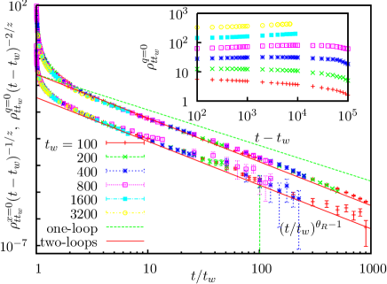
Figure 1: Scaling of the local $\rho^{x=0}_{tt_{w}}$ and the center of mass $\rho^{q=0}_{tt_{w}}$ integrated linear response functions of an elastic string relaxing at its depinning threshold (they have been shifted for clarity). The new critical exponent $\theta_{R}=-0.6\pm 0.05$ numerically obtained is in good agreement with our two-loop FRG prediction $\theta_{R}\approx-0.64$ (12). Here $z=1.5$ is the dynamical exponent, estimated numerically. Inset: non-scaled response data for the center of mass.

Dynamical properties are characterized by two-time $t,t_{w}$ response and correlation functions, describing the time evolution of the system as a function of its “age” or waiting-time $t_{w}$ from a given initial condition at $t=0$. Progress was achieved in the understanding of the steady-state, where these functions depend only on $t-t_{w}$. Functional Renormalization Group (FRG) calculations natterman ; Narayan and Fisher (1993); Chauve et al. (2000); ledoussal_frg_twoloops allowed to compute the critical exponents describing different universality classes, and powerful algorithms were developed to elucidate the low temperature dynamical phase diagram  Kolton et al. (2006a). In contrast, little is known about the more difficult transient regime, where the time-translation invariance is broken. Yet the first steps in that direction have unveiled rich and universal behaviors, including slow dynamics kolton_line_short_time and aging properties characterized by new exponents gregpld_epl .

Here we focus on elastic interfaces of dimension $d$ ($d=1$ for an elastic line) parameterized by a scalar field $u_{x,t}$ describing their position in a $d+1$-dimensional disordered medium. The driven overdamped dynamics of this model system obeys the equation of motion

$$\eta\partial_{t}u_{x,t}=c\nabla^{2}u_{x,t}+F(x,u_{x,t})+f\;,$$ (1)

where $\eta$ is the friction coefficient, $c$ the elastic constant, and $F(x,u)$ a quenched random pinning force with disordered averaged correlations $\overline{F(x,u)F(x^{\prime},u^{\prime})}=\Delta(u-u^{\prime})\delta^{d}(x-x^{\prime})$. Under an applied force $f$, the velocity is $v=L^{-d}\int d^{d}x\overline{\partial_{t}u_{x,t}}$. In this paper we consider a flat initial configuration $u_{x,t=0}=0$ but our results hold for any short ranged correlated initial conditions. Denoting $\hat{u}_{q,t}$ the spatial Fourier transform of $u_{x,t}$, we focus on the linear response ${\cal R}^{q}_{tt_{w}}$ to a small external field ${\hat{h}}_{-qt_{w}}$ and the correlation function ${\cal C}^{q}_{tt_{w}}$:

$${\cal R}^{q}_{tt_{w}}=\overline{\delta{\hat{u}}_{qt}/\delta{\hat{h}}_{-qt_{w}}}\quad,\quad{\cal{C}}^{q}_{tt_{w}}=\overline{{\hat{u}}_{qt}{\hat{u}}_{-qt_{w}}}\;.$$ (2)

The main result of this Letter is to establish, both via numerical calculations and additional analytical work, that these central observables take the scaling form:

$${\cal R}^{q}_{tt_{w}} = \left(t/t_{w}\right)^{\theta_{R}}q^{z-2}F_{R}[q^{z}(t-t_{w}),t/t_{w}]\;,$$ (3)

$${\cal C}^{q}_{tt_{w}} = q^{-(1+2\zeta)}(t/t_{w})^{\theta_{C}-1}F_{C}[q^{z}(t-t_{w}),t/t_{w}]\;,$$ (4)

with $\theta_{R}$ and $\theta_{C}$ two new universal critical exponents, i.e. independent of the usual depinning exponents. These are defined such that $F_{R,C}(y_{1},y_{2}\to\infty)\sim f_{R,C}(y_{1})$ for fixed $y_{1}$. In Eq. (3), (4), $F_{R,C}$ are universal scaling functions (up to a non universal amplitude) and $\zeta$ the roughness exponent. In the limit $y_{1}\to 0$, $y_{2}$ fixed, one finds $F_{R}(y_{1},y_{2})\sim y_{1}^{(2-z)/z}g_{R}(y_{2})$, $F_{C}(y_{1},y_{2})\sim y_{1}^{(d+2\zeta)/z}g_{C}(y_{2})$, i.e. a well defined $q\to 0$ limit. These scaling forms were predicted in Ref. gregpld_epl based on a one-loop FRG calculation. One may question however whether this lowest order in the $d=4-\epsilon$ dimensional expansion is accurate enough to describe interfaces of experimental interest $d=1,2$. In addition, no prediction for $\theta_{C}$ was obtained. Here we firmly establish that the above scaling forms hold and we provide a reliable determination of $\theta_{R}$ and $\theta_{C}$ in $d=1$. We also perform a two-loop FRG calculation, as is known to be required for a consistent theory of depinning ledoussal_frg_twoloops .

Most of the numerical studies of the transient dynamics have focused so far on one-time quantities which can be obtained from ${\cal{C}}^{q}_{tt^{\prime}}$ and ${\cal{R}}^{q}_{tt^{\prime}}$ in Eq. (3) and (4). The structure factor $S_{q}(t)\equiv{\cal{C}}^{q}_{tt}$ was found  kolton_line_short_time to behave as:

$$S_{q}(t)\equiv{\cal{C}}^{q}_{tt}\sim q^{-(d+2\zeta)}F[q{\ell}(t)]\;,\;\ell(t)\sim t^{1/z}\;,$$ (5)

where $F(y)\sim c^{\rm st}$, a constant, for $y\gg 1$ and $F(y)\sim y^{d+2\zeta}$ for $y\ll 1$. The relaxational dynamics is thus dictated by a single growing length, separating the small, steady-state equilibrated scales, from the large ones retaining a long-time memory of the initial condition. Eq. (5) is obtained from (4) in the limit $t\to t_{w}$ (i.e. $y_{2}\to 1$, $y_{1}\to 0$) with $q^{z}t$ (i.e. $y_{1}y_{2}/(y_{2}-1)$) fixed. The analogy with standard critical phenomena suggests for the velocity, the scaling form, $v(t,f)=b^{-\beta/\nu}G[b^{-z}t,b^{1/\nu}(f-f_{c}),b^{-1}L]$ where $b$ is an arbitrary rescaling factor, numerically verified in Ref. kolton_line_short_time . For $f=f_{c}$ and $t\ll L^{z}$ it implies that $v(t)\propto t^{-\beta/\nu z}$ and also that:

$$dv(t)/df\propto A\;t^{(2-z)/z}\;,$$ (6)

where we used the exact relations $\beta=\nu(z-\zeta)$ and $\nu=1/(2-\zeta)$, from statistical tilt symmetry (STS)  Narayan and Fisher (1993). We now check that this scaling of one time observables for $f=f_{c}$ is consistent with the two time scaling Eq. (4). Indeed Eq. (6) results by combining the exact relation Chauve et al. (2000) $\frac{d}{df}v(t)=\int_{0}^{t}ds\;\partial_{t}{\cal R}^{q=0}_{ts}$ and the limit $q\to 0$ of Eq. (3)

$${\cal R}^{q=0}_{tt_{w}}\sim(t-t_{w})^{(2-z)/z}\left(t/t_{w}\right)^{\theta_{R}}g_{R}(t/t_{w})\;,$$ (7)

with $g_{R}(x)\propto c^{\rm st}$ a constant for $x\gg 1$.

Let us now focus on two time quantities. To check Eqs. (3) and (4) we have performed numerical simulations of Eq. (1) in the case of elastic lines, $d=1$, experimentally relevant for many two dimensional systems, e.g. films. To study the non-stationary dynamics at $f=f_{c}$ we discretize Eq. (1) in the $x$ direction, $u_{x,t}\equiv u_{i}(t)$, with $i=0,...,L-1$, and use the method described in Ref. kolton_line_short_time . We start at $t=0$ with a flat configuration, $u_{i}(t=0)=0$, and monitor correlation and response functions at the exact sample critical force $f_{c}$  rosso . Numerically, it is more convenient to work with the local integrated response $\rho^{x=0}_{tt_{w}}\equiv\int_{0}^{t_{w}}ds\;\int_{q}{\cal R}_{ts}^{q}$ (where $\int_{q}$ denotes the integral over the first Brillouin zone) and zero-mode integrated response $\rho^{q=0}_{tt_{w}}\equiv\int_{0}^{t_{w}}ds{\cal R}_{ts}^{q=0}$. From Eq. (3) we predict,

$$\frac{\rho^{x=0}_{tt_{w}}}{(t-t_{w})^{1/z}}=h\left(\frac{t}{t_{w}}\right),\;\frac{\rho^{q=0}_{tt_{w}}}{(t-t_{w})^{2/z}}=\tilde{h}\left(\frac{t}{t_{w}}\right)\;,$$ (8)

where both $h(y)$ and $\tilde{h}(y)$ behave as $y^{-1+\theta_{R}}$ for $y\to\infty$. To implement the local (zero mode) response we define the observable $w_{i}(t)=u_{i}(t)-u_{cm}(t)$ ($w_{i}(t)=u_{i}(t)$) where $u_{cm}(t)\equiv\frac{1}{L}\sum_{i}u_{i}(t)$ and then compute,

$$\rho^{x=0(q=0)}_{tt_{w}}=\lim_{\alpha\rightarrow 0}\frac{1}{L}\sum_{i}\overline{[w_{i}(t)-w_{i}^{\alpha}(t)]\sigma_{i}}\alpha^{-1},$$ (9)

where $w_{i}^{\alpha}(t)$ is the solution of Eq. (1) with $u_{i}^{\alpha}(0)=u_{i}(0)=0$ and an additional perturbative force $\alpha\sigma_{i}\theta(t_{w}-t)$. We take random numbers $\sigma_{i}=\pm 1$ uncorrelated from site to site for computing $\rho^{x=0}_{tt_{w}}$, and $\sigma_{i}=\sigma_{0}$ for computing $\rho^{q=0}_{tt_{w}}$. The value of $\alpha$ is chosen small enough to guarantee linear response greg_superrough . In Fig. 1 we show the numerical results for $\rho^{x=0}_{tt_{w}}$ and $\rho^{q=0}_{tt_{w}}$, for $L=2048$ averaged over 10000 disorder realizations. We see that the predicted scaling forms, Eq. (8), describe well the data. For $t/t_{w}\gg 1$ we observe a well developed power law behavior with an aging exponent $\theta_{R}=-0.6\pm 0.05$ which is indistinguishable for both responses, $\rho^{x=0}_{tt_{w}}(t-t_{w})^{-1/z}\sim\rho^{q=0}_{tt_{w}}(t-t_{w})^{-2/z}\sim(t/t_{w})^{-1+\theta_{R}}$, as predicted. How does this numerical estimate for $\theta_{R}$ compare with the previous FRG approach of Ref. gregpld_epl ? The one loop result for $\theta_{R}=-\frac{\epsilon}{9}+{\cal O}(\epsilon^{2})$, setting $\epsilon=3$ gives $\theta_{R}\approx-1/3$. Incidentally, up to one loop order, one finds the relation $\theta_{R}=(z-2)/z$, which, using the numerical estimate $z=1.5$ kolton_line_short_time , yields again $\theta_{R}\approx-1/3$. Although it goes in the right direction, it is still far from our numerical result. To see whether the FRG predictions can be improved we have computed ${\cal R}^{q=0}_{tt_{w}}$ up to two loop order tbp . The starting point is Eq. (1). Response and correlations are then obtained from the standard dynamical (disorder averaged) Martin-Siggia-Rose action ${\cal S}$ which reads here

$${\cal S}=\int_{t>t^{\prime}>0}\int_{q}i\hat{u}_{qt}[(q^{2}+\partial_{t})\delta_{tt^{\prime}}+\hat{\Sigma}_{tt^{\prime}}]u_{-qt^{\prime}}$$

$$-\frac{1}{2}\int_{x,t>t^{\prime}>0}i\hat{u}_{xt}i\hat{u}_{xt^{\prime}}\Delta(u_{xt}-u_{xt^{\prime}})\;,$$ (10)

where $\Delta(u)$ is the force-force correlator and $\hat{\Sigma}_{tt^{\prime}}$ is the self-energy. As a result of the covariance of the action under STS Narayan and Fisher (1993) the self-energy has the structure $\hat{\Sigma}_{tt^{\prime}}=\Sigma_{tt^{\prime}}-\delta_{tt^{\prime}}\int_{0}^{t}dt_{1}\Sigma_{tt_{1}}$. It was computed to one loop in Ref. gregpld_epl and at two loop order the perturbation theory leads to diagrams similar to the one contributing the dynamical exponent $z$, as depicted in Fig. 10 of Ref. ledoussal_frg_twoloops , with the constraint that here, the time variables are positive. The (bare) response function ${\cal R}^{q}_{tt^{\prime}}=\langle i\hat{u}_{qt}u_{-qt^{\prime}}\rangle_{\cal S}$ is then computed from the exact identity

$${\cal R}^{q}_{tt^{\prime}}=R^{q}_{tt^{\prime}}-\int_{t^{\prime}<t_{1}<t_{2}<t}R^{q}_{tt_{2}}\Sigma^{q}_{t_{2}t_{1}}{\cal R}^{q}_{t_{1}t^{\prime}}$$

$$+\int_{t^{\prime}<t_{1}<t}R^{q}_{tt_{1}}{\cal R}^{q}_{t_{1}t^{\prime}}[\int_{0<t_{2}<t_{1}}\Sigma^{q}_{t_{1}t_{2}}]\;,$$ (11)

where $R^{q}_{tt^{\prime}}=\theta(t-t^{\prime})e^{-q^{2}(t-t^{\prime})}$ is the response in the absence of disorder.

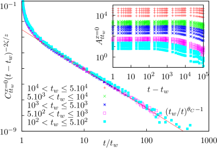
Figure 2: Scaling of the local autocorrelation function. The aging exponent is $\theta_{C}=-1.5\pm 0.05$, different from $\theta_{R}$. Inset: non-rescaled data.

Reexpressing in terms of $\Delta(u)$, corrected to the same order, and using the FRG fixed point equation, one explicitly shows that it has the scaling form as in Eq. (7). We then find that no new independent divergence occurs in $t/t^{\prime}$ at this order, hence that to two loop accuracy the relation $\theta_{R}=(z-2)/z+{\cal O}(\epsilon^{3})$ continues to hold. Our numerical result however indicates that this relation cannot hold to all orders in $\epsilon$, i.e one must have $\theta_{R}\neq(z-2)/z$, implying that $\theta_{R}$ is indeed a new independent exponent. One way to understand the FRG result is then to rewrite more explicitly,

$$\theta_{R} = -\frac{\epsilon}{9}+\left(\frac{1}{162\gamma\sqrt{2}}-\frac{\log{2}}{108}-\frac{23}{648}\right)\epsilon^{2}+O(\epsilon^{3})$$ (12)

$$= -0.1111...\epsilon-0.03395...\epsilon^{2}+O(\epsilon^{3})\;,$$

with $\gamma=0.54822..$. We note that if we set $\epsilon=3$ in that expression (12) assuming the $O(\epsilon^{3})$ to be small, we obtain $\theta_{R}=-0.64...$, very close to the the numerical value. Hence we conclude that although corrections to 3 loop and higher to $\theta_{R}-(z-2)/z$ must be large, in $\theta_{R}$ they must be small. This provides one way of interpreting our results, and motivation for future analytical work.

We have also checked numerically the scaling form for the correlation function in Eq. (4). It is more convenient to compute the autocorrelation function ${\cal C}^{x=0}_{tt_{w}}=\overline{u_{x,t}u_{x,t_{w}}}$ obtained from ${\cal C}^{q}_{tt_{w}}$ by integration over Fourier modes ${\cal C}^{x=0}_{tt_{w}}=\int_{q}{\cal C}^{q}_{tt_{w}}$. From Eq. (4), one expects ${\cal C}^{x=0}_{tt_{w}}\sim(t-t_{w})^{2\zeta/z}\hat{h}\left(t/t_{w}\right)$ where $\hat{h}(y)\propto y^{-1+\theta_{C}}$ for large $y$. To check this, we compute numerically ${\cal C}^{x=0}_{tt_{w}}=L^{-1}\sum_{i}\overline{w_{i}(t)w_{i}(t^{\prime})}$. In Fig. 2 we show a plot of $(t-t_{w})^{-2\zeta/z}{\cal C}^{x=0}_{tt_{w}}$ for $L=2048$ obtained by averaging over 10000 samples, which is in good agreement with the predicted scaling. For $t/t_{w}\gg 1$, we see a power-law behavior with a non-equilibrium exponent $\theta_{C}=-1.5\pm 0.05$. At variance with pure critical dynamics calabrese_review , one obtains that $\theta_{C}$ and $\theta_{R}$ are different exponents. Such behavior was observed in other disordered elastic systems (though relaxing at equilibrium) co_pre . The determination of $\theta_{C}$ via the FRG requires a computation to order ${\cal O}(\epsilon^{2})$ of ${\cal C}^{q}_{tt_{w}}$ and remains a challenge.

So far we have analyzed the situation where $\ell(t)<L$. Finite-size effects can be observed in experiments however, as shown recently for domain walls in magnetic nanowires Kim et al. (2009), and vortex lattices in micron-sized superconductors moira . The finite-size crossover manifests in the velocity as $v(t)L^{\beta/\nu}=f(t/L^{z})$ and for $t>L^{z}$ the interface losts memory of the initial condition kolton_line_short_time .

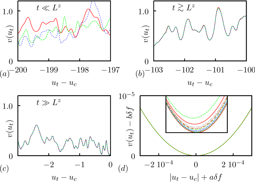
Figure 3: (a-c) Three different initial conditions evolving at $f_{c}$ in the same sample coalesce into a unique reparametrized velocity function $v(u_{cm}(t))$ after a typical time $t\sim L^{z}$, before stoping at the critical configuration, $u_{c}\equiv u_{cm}(\infty)$. (d) The steady-state structure of $v(u_{cm})$ around $u_{c}$ for different forces $\delta f\equiv f-f_{c}\to 0^{+}$ is a well defined parabola with a positive (negative) shift proportional to $\delta f$ in the position (velocity) axis. Inset: unshifted data. One finds for $L=32$ and $\delta f/f_{c}=6-13,20,30\;10^{-6}$ $a\approx 0.16$, $b\approx 1.45$.

What happens next? Remarkably, a detailed analysis of the dynamics for $t>L^{z}$ reveals that different initial conditions in the same sample evolve collapsing into a unique, sample-dependent, reparametrized velocity $v(u_{cm})$ (as a function of the center of mass position), before stopping at the critical configuration, as shown in Fig. 3(a-c). This behaviour can be seen as a direct consequence of the Middleton theorems, which assures the convergence to a unique periodic attractor for $f\geq f_{c}$ Middleton (1992). For $t\gg L^{z}$ we can thus describe the velocity by an effective equation of motion for a particle, $\dot{u}_{t}=v(u_{t},f)$ with $u_{t}\equiv u_{cm}(t)$.

Before exploring further the consequences, let us note that the $d=0$ problem of a particle is a solvable limit, interesting per se, as the (sample dependent) response function is given exactly by  chauve_thesis $R_{tt_{w}}=\theta(t-t_{w})v(u_{t},f)/v(u_{t_{w}},f)$. In the usual model $\eta v(u_{t},f)=F(u_{t})+f$, near the threshold, $\delta f=f-f_{c}\ll f_{c}$, the particle spends most time near the zero force point (set to be at $u=0$). For a smooth force field we can write $\eta\dot{u}_{t}=\gamma u^{2}_{t}+\delta f$ which yields $v(t)\sim t^{-2}$ and

$$R_{tt_{w}}=\theta(t-t_{w})\begin{cases}\frac{\sin^{2}{(t_{w}\sqrt{\gamma\delta f}/\eta)}}{\sin^{2}{(t\sqrt{\gamma\delta f}/\eta)}}\;,\;\delta f>0\\ \frac{\sinh^{2}{(t_{w}\sqrt{\gamma|\delta f|}/\eta)}}{\sinh^{2}{(t\sqrt{\gamma|\delta f|}/\eta)}}\;,\;\delta f<0\\ \left(t/t_{w}\right)^{-2}\end{cases}$$ (13)

for $\delta f\to 0$. Hence $\theta_{R}(d=0)=-2$, consistent with a monotonic dependence of $\theta_{R}$ with $d$, and $\beta(d=0)=1/2$.

Next, we confirm that the results of the $d=0$ model are relevant for the interface for $\ell(t)>L$. As shown in Fig. 3d, we checked that for interfaces of sizes $L=32$ and small $\delta f\ll f_{c}$ the reparametrized velocity has a nice parabolic shape near the zero force point, $v(u,f)=\gamma(u+a\delta f)^{2}+b\delta f$ where the constants $b,\gamma>0$ (their size dependence will be studied elsewhere tbp ). $a$ being found irrelevant, this result is consistent with the steady-state value $\beta=1/2$ found for the interface in the regime $\delta f^{-\nu}\gg L$ duemmer_crossover , and predicts a crossover to an effective $\theta_{R}^{eff}=-2$ in the fixed $L$, large $t$ limit for the interface.

For modeling contact lines  Moulinet et al. (2004) the term $\nabla^{2}u_{x,t}$ in Eq.(1) is replaced by a long range elastic force $\int_{x^{\prime}}[u(x^{\prime},t)-u(x,t)]/|x-x^{\prime}|^{2}$. In this case, using the same numerical method, we confirm the scaling forms (3) (replacing $q^{z-2}\to q^{z-1}$) and measure $\theta_{C}=-1.2\pm 0.1$ and $\theta_{R}=-0.5\pm 0.1$. The same analysis leading to (12) gives $\theta_{R}=-0.22$ to one loop and $\theta_{R}=-0.38$ to two loop.

To conclude we have confirmed numerically the scaling forms for non stationary dynamics at depinning, for model systems of experimental relevance. The exponent $\theta_{R}$ is found in reasonable agreement with FRG predictions. An interesting dimensional crossover was found at large time. We hope this motivates new experiments, e.g in magnets and wetting.

This work was supported by the France-Argentina MINCYT-ECOS A08E03. A.B.K aknowledges the hospitality at LPT-Orsay and ENS-Paris.

References

(1)
(2)
(3)
(4)
(5)
(6)
(7)
(8)
(9)
(10)
(11)
Lemerle et al. (1998)S. Lemerle et al.,
Phys. Rev. Lett.
80, 849 (1998).
Repain et al. (2004)
V. Repain et al.,
Europhys. Lett. 68,
460 (2004).
Metaxas et al. (2007)
P. J. Metaxas et al.,
Phys. Rev. Lett. 99,
217208 (2007).
Kim et al. (2009)
K.-J. Kim,
et al., Nature
458, 740 (2009).
Paruch et al. (2005)
P. Paruch,
T. Giamarchi,
and J. M.
Triscone, Phys. Rev. Lett.
94, 197601
(2005).
Tybell et al. (2002)
T. Tybell et al., Phys. Rev. Lett.
89, 097601
(2002).
Moulinet et al. (2004)
S. Moulinet et al.,
Phys. Rev. E 69,
035103(R) (2004).
(19)
P. Le Doussal et al., Preprint arXiv:0904.4156.
Ponson et al. (2006)
L. Ponson,
D. Bonamy, and
E. Bouchaud,
Phys. Rev. Lett. 96,
035506 (2006).
Alava et al. (2006)
M. Alava,
P. K. V. V. Nukalaz,
and S. Zapperi,
Adv. Phys. 55,
349 (2006).
Fisher (1985)
D. S. Fisher,
Phys. Rev. B 31,
1396 (1985).
(23)
G. Schehr, P. Le Doussal, Europhys. Lett. 71(2), 290 (2005).
(24)
A. B. Kolton et al., Phys. Rev. B 74,
140201(R) (2006) .
(25)
L. F. Cugliandolo, Dynamics of glassy systems in Slow relaxation and nonequilibrium
dynamics in condensed matter, J. L. Barrat et al., Springer-Verlag, 2002.
(26)
P. Calabrese, A. Gambassi, J.Phys. A 38, R133 (2005).
Narayan and Fisher (1993)
O. Narayan and
D.S. Fisher,
Phys. Rev. B 48,
7030 (1993).
(28)
T. Nattermann et al., J. Phys. II (France) 2 (1992) 1483
Chauve et al. (2000)
P. Chauve,
T. Giamarchi,
and P. Le
Doussal, Phys. Rev. B 62,
6241 (2000).
(30)
P. Chauve, P. Le Doussal and K.J. Wiese, Phys. Rev. Lett. 86, 1785 (2001);
P. Le Doussal, K.J. Wiese and P. Chauve, Phys. Rev. B 66, 174201 (2002)
Kolton et al. (2006a)
A. B. Kolton et al.,
Phys. Rev. Lett. 97,
057001 (2006a);
Phys. Rev. B 79,
184207 (2009a).
(32)
A. Rosso and W. Krauth Phys. Rev. Lett. 87,187002 (2001);
Phys. Rev. B 65, 012202 (2001);
A. Rosso, A. Hartmann and W. Krauth;
Phys. Rev. E 67, 021602 (2003).
(33)
G. Schehr and H. Rieger, Phys. Rev. B 71, 184202 (2005).
(34)
O. Duemmer and W. Krauth, Phys. Rev. E 71, 061601 (2005); cond-mat/0501467.
(35)
Details will be published elsewhere.
(36)
M. I. Dolz, A. B. Kolton, H. Pastoriza, unpublished.
Middleton (1992)
A. A. Middleton,
Phys. Rev. Lett. 68,
670 (1992).
(38)
G. Schehr and P. Le Doussal, Phys. Rev. E 68, 046101 (2003).