NMR multiple quantum coherences in quasi-one-dimensional spin systems:
Comparison with ideal spin-chain dynamics

Abstract

The ¹⁹F spins in a crystal of fluorapatite have often been used to experimentally approximate a one-dimensional spin system. Under suitable multi-pulse control, the nuclear spin dynamics may be modeled to first approximation by a double-quantum one-dimensional Hamiltonian, which is analytically solvable for nearest-neighbor couplings. Here, we use solid-state nuclear magnetic resonance techniques to investigate the multiple quantum coherence dynamics of fluorapatite, with an emphasis on understanding the region of validity for such a simplified picture. Using experimental, numerical, and analytical methods, we explore the effects of long-range intra-chain couplings, cross-chain couplings, as well as couplings to a spin environment, all of which tend to damp the oscillations of the multiple quantum coherence signal at sufficiently long times. Our analysis characterizes the extent to which fluorapatite can faithfully simulate a one-dimensional quantum wire.

I Introduction

Low-dimensional quantum spin systems are the subject of intense theoretical and experimental investigation. From a condensed matter perspective, not only do these systems provide a natural setting for deepening the exploration of many-body quantum coherence properties as demanded by emerging developments in spintronics and nanodevices Awschalom07 ; Childress et al. (2006); Dutt07 , but the ground states of one-dimensional (1D) conductors provide insight into the solution of the one-band Hubbard Hamiltonian Essler05 . From a quantum information perspective Nielsen and Chuang (2000), quantum spin chains have been proposed as quantum wires for short-distance quantum communication, their internal dynamics providing the mechanism to coherently transfer quantum information from one region of a quantum computer to another Bose03 (see also Bose08 for a recent overview). Perfect state transfer, in particular, has been shown to be theoretically possible by carefully engineering the couplings of the underlying spin Hamiltonian. A number of efforts are underway to devise protocols able to achieve reliable quantum information transfer under more realistic conditions – bypassing, for instance, the need for initialization in a known pure state DiFranco08 , explicitly incorporating the effect of long-range couplings Kay06 ; Avellino06 ; Gualdi08 , or exploiting access to external end gates Burg06 ; Zhang09 . Still, few (if any) physical systems can meet the required constraints, and it is likely that quantum simulators will be needed to experimentally implement these schemes. Of course, quantum simulators will in turn allow us to probe a much broader range of questions encompassing both quantum information and condensed matter physics Lloyd96 . Optical lattices have shown much promise in simulating quantum spin systems Bloch08 . Among solid-state devices, coupled spins in apatites have recently enabled experimental studies of 1D transport and decoherence dynamics Cho06 ; Cappellaro et al. (2007a, b); Oliva08 .

Fluorapatite (FAp) has long been used as a quasi-1D system of nuclear spins. Lowe and co-workers characterized the nuclear magnetic resonance (NMR) line shape of FAp Engelsberg73 ; Sur75a , and described the dipolar dynamics of the free induction decay in terms of the 1D XY model Sur75b . Cho and Yesinowski investigated the many-body dynamics of FAp under an effective double-quantum (DQ) Hamiltonian, and showed that the growth of high-order quantum coherences was distinctly different from that obtained in dense 3D crystals Cho93 ; Cho and Yesinowski (1996). From a theoretical standpoint, FAp provides a rich testbed to explore the controlled time evolution of a many-body quantum spin system. The DQ Hamiltonian is analytically solvable in the tight-binding limit, where only nearest neighbor (NN) couplings are present Feldman and Lacelle (1997); Doronin00 ; Cappellaro et al. (2007a). Previous work showed that the implementation of a DQ Hamiltonian in the FAp system using coherent averaging techniques is a promising tool for the study of transport in quantum spin chains. We demonstrated, in particular, that the DQ Hamiltonian is related to the XY-Heisenberg Hamiltonian by a similarity transformation, and that it is possible to transfer polarization from one end of the chain to the other under the DQ Hamiltonian Cappellaro et al. (2007b). In fact, the signature of this transport shows up in the collective multiple quantum coherence (MQC) intensity of the spin chain. Experimentally, it has also been shown that it is possible to prepare the spin system in an initial state in which the polarization is localized at the ends of the spin chain Cappellaro et al. (2007a), paving the way towards achieving universal quantum control Fitzsimons06 .

Since the mapping between the experimental system and the idealized model Cappellaro et al. (2007a, b) is not perfect, an essential step forward is to address where and how this model breaks down, which constitutes the main aim of this paper. In particular, we systematically examine the viability of using NMR investigations of FAp as a test-bed for 1D transport, by relying on a combination of experimental and numerical methods. We first examine the effects on the relevant observables of experimental errors introduced during the implementation of the DQ Hamiltonian, which arise due to higher-order terms in the average Hamiltonian describing the effective spin evolution. We also examine errors introduced in some state initialization sequences due to the restriction of the control fields to collective rotations. Since the FAp crystal is in reality a three-dimensional (3D) lattice, we next investigate in detail how the spin dynamics is affected by the presence of longer-range couplings, both within a single chain and between adjacent spin chains.

The content of the paper is organized as follows. We describe the quasi-1D spin system of FAp in Sec. II, including the evolution in the absence of control as well as the dynamics under suitable pulse sequences. In the same section, we also discuss the system initialization and the readout of the experimental MQC signal. Sections III and IV present both experimental and numerical results of MQC dynamics, and are the core of the paper. By comparing the numerical results with the analytical predictions available in the limiting case of a DQ Hamiltonian with NN couplings, we evaluate the effect of high-order average Hamiltonian terms, next-nearest-neighbor (NNN) couplings, and cross-chain couplings between multiple chains. Our findings are summarized in Sec. V. Appendix A presents technical background on the relevant numerical methodology, whereas we also include in Appendix B a description of finite size effects as found in simulations, and in Appendix C a discussion of an alternative chaotic model for the spin bath.

II Physical system and experimental settings

II.1 Spin Hamiltonian of fluorapatite

We consider a single crystal of FAp [Ca₅(PO₄)₃F] at room temperature, placed in a strong external magnetic field along the $z$-direction that provides the quantization axis for the nuclear spins. It is possible to truncate the magnetic dipolar interaction among the spins in this strong field, keeping only the secular terms. The resulting secular dipolar interaction Slichter (1992) among $N$ ¹⁹F nuclear spin-1/2 is anisotropic due to the presence of the quantization field, leading to a Hamiltonian of the form:

$${\cal H}_{dip} = \sum_{j<\ell}^{N}b_{j\ell}\left[\sigma^{z}_{j}\sigma^{z}_{\ell}-\frac{1}{2}(\sigma^{x}_{j}\sigma^{x}_{\ell}+\sigma^{y}_{j}\sigma^{y}_{\ell})\right].$$ (1)

Here, $\sigma_{j}^{\alpha}$ ($\alpha=x,y,z$) denotes the Pauli matrices of the $j$th spin and $b_{j\ell}=(\mu_{0}/16\pi)(\gamma^{2}\hbar/r_{j\ell}^{3})(1-3\cos^{2}\theta_{j\ell})$, with $\mu_{0}$ the standard magnetic constant, $\gamma$ the gyromagnetic ratio of fluorine, $r_{j\ell}$ the distance between nucleus $j$ and $\ell$, and $\theta_{j\ell}$ the angle between $\vec{r}_{j\ell}$ and the $z$-axis. The geometry of the spin system is reflected in the distribution of the $b_{j\ell}$ couplings.

The FAp crystal has a hexagonal geometry with space group P$6_{3}$/m Van Der Lugt and Caspers (1964) (see Fig. 1.a). The dimensions of the unit cell are $D=9.367$ Å and $c=6.884$ Å. The ¹⁹F nuclei form linear chains along the $c$-axis, each one surrounded by six other chains. The distance between two intra-chain ¹⁹F nuclei is $d=c/2=3.442$ Å  and the distance between two cross-chain ¹⁹F nuclei is $D$. The largest ratio between the strongest intra- and cross- chain couplings ($\approx 40$) is obtained when the crystalline $c$-axis is oriented parallel to the external field. Thus, to a first approximation, in this crystal orientation the 3D ¹⁹F system may be treated as a collection of many identical 1D chains. For a single chain oriented along $z$, we have $b_{j\ell}=-(\mu_{0}/\pi)(\gamma^{2}\hbar/c^{3}|j-\ell|^{3})$.

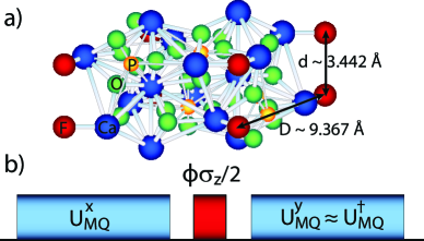
Figure 1: a) Unit cell of the fluorapatite crystal [Ca₅(PO₄)₃F], highlighting the geometry of the fluorine chains (in red). b) NMR pulse sequence for the creation and detection of MQC.

In reality, naturally occurring defects in the sample (such as vacancies or substitutions FapDefects ) cause the chains to be broken into many shorter chains. Here we model the system as an ensemble of (approximately) independent and equivalent chains with finite length. Such a simplified description is necessary to obtain a computationally tractable model.

II.2 Control capabilities and effective dynamics

II.2.1 Unitary control

Unitary control is obtained by applying (near)resonant radio-frequency (rf) pulses to the spin system. FAp contains ¹⁹F and ³¹P spins-$1/2$, both of which are 100% abundant. Moreover, in an ideal crystal, all the ¹⁹F spins are chemically equivalent, as are all the ³¹P spins. As a consequence, all rf control pulses are applied collectively to all the spins.

In NMR, the term MQC refers to coherences between two or more spins. When the system is quantized along the $z$-axis, a quantum coherence of order $n$ is associated to the transition between two states $|m_{1}\rangle$ and $|m_{2}\rangle$, such that the difference of the magnetic moment along $z$ of these states $(m_{1}-m_{2})\propto n$. That is, multiple quantum coherences of order $n$ describe states like $|m_{2}\rangle\langle m_{1}|$, or elements in the density matrix that correspond to a transition between these two states MQCbook . Quantum coherences can also be classified based on their response to a rotation around the $z$ (quantization) axis. A state of coherence order $n$ acquires a phase proportional to $n$ under a $z$-rotation. Multiple quantum NMR techniques Hatanaka75 ; Pines76 ; Aue76 ; Vega76 ; Warren80 have enabled researchers to probe multi-spin processes, and gain insight into the many-body spin dynamics of dipolar-coupled solids Baum85 ; Munowitz87b ; Levy92 ; Lacelle93 ; Ramanathan et al. (2003); Cho05 ; Cho06 .

To study the MQC dynamics of the spin system, we typically let it evolve under the DQ Hamiltonian

$${\cal H}_{DQ} = \sum_{j<\ell}\frac{b_{j\ell}}{2}(\sigma^{x}_{j}\sigma^{x}_{\ell}-\sigma^{y}_{j}\sigma^{y}_{\ell})$$ (2)

$$= \sum_{j<\ell}b_{j\ell}(\sigma^{+}_{j}\sigma^{+}_{\ell}+\sigma^{-}_{j}\sigma^{-}_{\ell}),$$

with $\sigma_{j}^{\pm}=(\sigma_{j}^{x}\pm i\sigma_{j}^{y})/2$. Following Baum85 ; Ramanathan et al. (2003), we utilize a $16$-pulse cycle applied on-resonance with the ¹⁹F Larmor frequency to implement the DQ Hamiltonian to lowest order in AHT description Slichter (1992); Haeberlen (1976); AHTnote . A key feature of this sequence is that the fluorine-phosphorus dipolar interaction is decoupled, which makes it possible to ignore the presence of the ³¹P spins in the rest of this paper. The dynamics during the pulse sequence can be written in terms of an effective Hamiltonian $\overline{\mathcal{H}}_{DQ}$,

$$U^{x(y)}_{MQ}(t) = \mathcal{T}\exp\left(-i\int_{0}^{t}[\mathcal{H}_{dip}+{\cal H}^{x(y)}_{rf}(s)]ds\right)$$ (3)

$$= e^{\pm i\overline{\mathcal{H}}_{DQ}t},$$

where $\mathcal{T}$ denotes time-ordering operator, $\hbar=1$, and ${\cal H}_{rf}^{x(y)}(t)$ is the time-dependent Hamiltonian describing the rf-pulses along the $x$- (or $y$-) axis (whereby the corresponding $\pm$ sign in front of the effective Hamiltonian).

II.2.2 Initialization capabilities

The spin dynamics under the DQ Hamiltonian depends critically on the initial state in which the system is prepared. Here, we focus our attention on two choices of direct experimental relevance Cappellaro et al. (2007a). One is the equilibrium Zeeman thermal state, which is obtained at the thermal equilibrium in a strong external magnetic field ($B_{0}=7$ T in our experiments) at room temperature. The thermal state can be expressed as

$$\rho^{\prime}_{th}(0) \propto \exp(-\varepsilon\sigma_{z})\approx\openone-\varepsilon\sigma_{z},$$ (4)

where $\sigma_{z}=\sum_{j}\sigma_{j}^{z}$ and $\varepsilon=\gamma B_{0}/k_{B}T$, with $k_{B}$ the Boltzmann constant and $T$ the temperature ($\varepsilon\approx 10^{-5}$ at room temperature for FAp). In line with standard NMR practice, we consider only the evolution due to the component proportional to $\varepsilon$, $\rho_{th}(0)=\sigma_{z}$, since the identity matrix does not evolve or contribute to the MQC signal under the assumption of unital dynamics. The second initial state that is experimentally available is a mixture of states where only a spin at the extremities of the chain is polarized, which can be formally represented as

$$\rho_{end}(0) = \sigma^{z}_{1}+\sigma^{z}_{N},$$ (5)

where spin 1 and spin $N$ are located at the two ends of the spin chain Cappellaro et al. (2007a). We refer to this as the end-polarized state. A description of the method used to create this state is given in Sec. IV.1.2.

II.2.3 Readout capabilities

In an inductively detected NMR experiment (in which a coil is used to measure the average magnetization), the observed signal is $S(t)=\zeta\langle\sigma^{-}(t)\rangle=\zeta\mathrm{Tr}\left\{\sigma^{-}\rho(t)\right\}$, where $\sigma^{-}=\sum_{j}\sigma_{j}^{-}$ and $\zeta$ is a proportionality constant. The only terms in $\rho(t)$ that yield a non-zero trace, and therefore contribute to $S(t)$, are angular momentum operators such as $\sigma_{j}^{+}$, which are single-spin, single-quantum coherences. Thus, in order to characterize multi-spin dynamics, it is necessary to indirectly encode the signature of the dynamics into the above signal. This is precisely what is done in standard NMR MQ spectroscopy, using an evolution-reversal experiment MQCbook . The density operator at the end of an MQ experiment is given by

$$\rho_{f}=U_{MQ}^{\dagger}U_{\textrm{evol}}U_{MQ}\rho_{i}U_{MQ}^{{\dagger}}U_{\textrm{evol}}^{\dagger}U_{MQ},$$ (6)

where $U_{MQ}=\exp(-i{\cal H}_{DQ}t)$, and $U_{\textrm{evol}}$ determines the nature of the information encoded (see Fig. 1.b).

In our experiment, we are interested in the evolution of MQC under the DQ Hamiltonian, thus we measure the signal as we systematically increase $t$. In order to encode information about the distribution of the MQC, we apply a collective rotation about the $z$ quantization axis, $U_{\textrm{evol}}=\exp(-i\phi\sigma_{z}/2)$. Then, to extract the coherence order distribution, the measurement is repeated while incrementing $\phi$ from 0 to $2\pi$, in steps of $\delta\phi=2\pi/2K$, where $K$ is the highest order of MQC encoded. The signal acquired in the $k$-th measurement is then $S_{z}^{k}(t)={\rm Tr}[\rho^{k}(t)\sigma_{z}]$, where $\rho^{k}(t)$ is the density matrix evolved under the propagator $U_{k}(t)=e^{i\overline{\mathcal{H}}_{DQ}t}e^{-ik\delta\phi\sigma_{z}/2}e^{-i\overline{\mathcal{H}}_{DQ}t}$, and we have assumed that $\sigma_{z}$ is the experimental observable. In practice, we use either a $\pi/2$ pulse or a solid echo SolidEcho to read out the signal at the end of the experiment. Fourier-transforming the output with respect to $\phi$ yields the coherence order intensity:

$$J_{n}(t) = \sum_{k=1}^{K}S_{z}^{k}(t)e^{-ikn\delta\phi}.$$ (7)

Note that since the initial states we consider are population terms in the $z$-basis, the final states at the end of the evolution-reversal experiment are also population terms (hence our use of the observable $\sigma_{z}$).

III Multiple quantum dynamics: Simple model and experiment

III.1 Ideal spin-chain dynamics

The fact that the evolution of the 1D spin chain under a DQ Hamiltonian is exactly solvable in the tight binding limit Feldman and Lacelle (1997); Doronin00 ; Cappellaro et al. (2007a) provides a useful starting point for theoretical analysis. Hereafter, we shall refer to this model as the analytical model. Moreover, the DQ Hamiltonian is related to the XY Hamiltonian by a similarity transformation that inverts every alternate spin in the chain Doronin00 ; Cappellaro et al. (2007b). Besides using the analytical results to calibrate our numerical methods (see Appendix A), we will also investigate the effect of long-range interactions beyond the NN limit, by comparing numerical and analytical results. For convenience, we set the NN coupling strength in the DQ Hamiltonian of Eq. (2) $b\equiv b_{12}=1$, so that time shall be measured in units of $1/b$ henceforth (unless explicitly stated otherwise).

For both the thermal and the end-polarized initial state, only zero and DQ coherences are predicted by the analytical model. Specifically, for the thermal initial state, the normalized intensities are

$$J_{0}^{th}(t) = \frac{1}{N}\sum_{k}\cos^{2}(4bt\cos\psi_{k}),$$

$$J_{2}^{th}(t) = \frac{1}{2N}\sum_{k}\sin^{2}(4bt\cos\psi_{k}),$$ (8)

where as before $N$ is the number of spins in the chain and $\psi_{k}=k\pi/(N+1)$. For the end-polarized initial state,

$$J_{0}^{end}(t) = \frac{2}{N+1}\sum_{k}\sin^{2}(\psi_{k})\cos^{2}(4bt\cos\psi_{k}),$$

$$J_{2}^{end}(t) = \frac{1}{N+1}\sum_{k}\sin^{2}(\psi_{k})\sin^{2}(4bt\cos\psi_{k}).$$ (9)

In both Eqs. (8)-(9), the normalization is chosen such that $J_{0}+2J_{2}=1$.

III.2 Experimental results

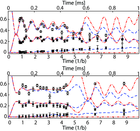
Figure 2: (Color online) Experimental data (0Q circles, 2Q-stars, 4Q squares), analytical results (red dash-dotted lines), and least square fit (blue dashed lines) of experimental data to numerical calculations under the DQ Hamiltonian with NN and NNN couplings of strength $b$ and $b/8$, respectively. Error bars for the experimental data were estimated from the standard deviation of the odd quantum coherences from zero. Numerically, two free parameters, the time origin $t_{0}$ and the time scale $1/b$, are adjusted to obtain the best fit to the experimental data for $J_{0}$. Top: Thermal initial state with chain length $N=18$. Fitting parameters $t_{0}=9.6\mu$s and $1/b=101.8\mu$s. Bottom: End-polarized initial state wth chain length $N=19$. Fitting parameters $t_{0}=0.2\mu$s and $1/b=100.8\mu$s.

The experiments were performed in a 7 T magnetic field using a Bruker Avance Spectrometer equipped with a home-built probe. The ¹⁹F frequency is 282.37 MHz. Experimentally measured MQC data are shown in Fig. 2, along with analytical predictions and simulation results under the DQ Hamiltonian with NN and NNN couplings. Both the time origin $t_{0}$ and the coupling strength $b$ were used as fitting parameters in order to minimize the square of the difference between the experimental and numerical data, that is, $\sum_{i}\left|J_{0}^{\text{exp}}(t_{i})-J_{0}^{\text{num}}[b(t_{i}-t_{0})]\right|^{2}$. For the thermal initial state data (upper row in Fig. 2), the $\pi/2$ pulse length was 1.05 $\mu$s, the inter-pulse delay $\Delta$ was varied from 2.9 to 5 $\mu$s, and the number of loops was increased from 1 to 7. We set $K=12$, and incremented the phase in steps of $2\pi/24$ to encode the MQCs. For the end-chain initial state data (lower row in Fig. 2), the $\pi/2$ pulse length was 0.93 $\mu$s, the end-state preparation time $t_{1}=30.3\>\mu$s, the inter-pulse delay $\Delta$ was varied from 2.9 to 7.3 $\mu$s, and the number of loops increased from 1 to 8. We set $K=16$, and incremented the phase in steps of $2\pi/32$ to encode the MQCs. In both cases, the recycle delay was 300s and a solid echo sequence with an 8-step phase cycle was used to read out the signal intensities at the end of the experiment.

The experimental data are normalized at every time step, such that $J_{0}+2(J_{2}+J_{4})=1$ (using the fact that $J_{-n}=J_{n}$). The intensities of the odd MQCs (not shown in Fig. 2) turn out to be negligibly small. At short times (less than $\approx 0.2$ ms), Fig. 2 indicates that fourth- and higher-order even-MQCs are also negligible. However, the four-quantum coherence signal contributes significantly at longer times. In 3D systems, including both plastic crystals such as adamantane Suter04 and rigid crystals such as the cubic lattice of ¹⁹F spin in CaF₂ Levy92 ; Cho05 , very high coherence orders are seen to develop over a time scale less than a millisecond, with no apparent restriction on the highest order reached. In contrast, the fact that the MQ intensities are restricted to the zero- and DQ-coherences, and that the higher-order terms only grow relatively slowly during the whole time domain we explored, are strong indications of the 1D character of the spin system. At the same time, the appreciable intensity of the four-quantum coherence at long evolution times clearly indicates that the analytical model (which predicts only zero- and DQ- coherences for both the thermal and end-polarized initial states) becomes inadequate to accurately describe the real system.

Note that in the simulations, the maximum computationally accessible chain length was $N=21$ spins. Though the fits included in Fig. 2 use $18$-$19$ spins, it is important to realize that sensitivity of the dynamics to the precise value of $N$ develops only at sufficiently long times (as the effect of the finite chain boundaries manifest – see Appendix B), where the accuracy of the simple model used to make the estimate becomes itself limited.

IV Multiple quantum dynamics: Beyond spin-chain approximation

In order to understand the discrepancies observed between the analytical model and the experimental results, it is necessary to identify the dominant sources of non-ideality in the experiment, and assess their respective effects on the observables under examination. With this in mind, we first analyze effects due to limited control, such as the higher-order terms in AHT as well as imperfect system initialization. We then investigate the intrinsic limitations of the 1D NN model to describe the real physical system, which contains an ensemble of weakly-coupled spin chains with long-range intra-chain couplings. In particular, we compare the effects of long-range interactions first within a single chain and then across different spin chains. Note that while long-range couplings have been previously accounted for in a perturbative limit Feldman and Lacelle (1997), we resort here to exact numerical simulations (Appendix A), while also considering other experiment-related sources of errors.

IV.1 Errors due to limited control

IV.1.1 High-order terms in Average Hamiltonian Theory

As mentioned, experimentally the DQ Hamiltonian (2) is obtained as the zeroth order average Hamiltonian of a multiple-pulse sequence. Since the 16-pulse cycle used in the experiment is time-symmetric Ramanathan et al. (2003), all odd-order corrections are zero, and the leading error term is of second-order in $\left\|\bar{\cal H}^{(2)}T_{c}\right\|$, both when considering ideal and finite-width pulses. The contributions to the effective Hamiltonian from higher-order terms may be estimated by comparing the single-cycle MQC signal computed using the exact DQ Hamiltonian, and using the dipolar Hamiltonian (1) interspersed with rf pulses, respectively. Assuming ideal instantaneous pulses, we verified numerically that for the system of interest such contributions are small provided that the cycle time $T_{c}\lesssim 4$ (see Fig. 3, Inset). In the experiment, we thus employed multi-cycle sequences, in order to extend the region of validity of the DQ model.

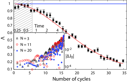
Figure 3: (Color online) Overlap $\Lambda$ for end-polarized initial state, Eq. (10). Normalized experimental data (stars) and numerical results for finite-width pulses (solid line). The chain length in the numerical calculation is $N=9$, whereas the pulse length and inter-pulse delay are $w=0.0075\,b\approx 1\mu$s and $\Delta=0.0225\,b$, respectively, which are close to the experimental values. The shaded area is the time region explored in the MQC experiments. Inset: Absolute value of the difference between $J_{0}$ as calculated from the analytical model or the rf-pulsed dipolar Hamiltonian with the initial thermal state under different chain lengths, as a function of cycle time. Only NN couplings are considered in this case.

In order to determine how well we implemented the evolution reversal experiment described in Sec. II, we performed a series of experiments that measured the overlap between the initial and the final state, following evolution reversal. This overlap is given by

$$\Lambda={\rm Tr}[\rho_{th}U_{MQ}^{y}U_{MQ}^{x}\rho_{end}(0)U_{MQ}^{x{\dagger}}U_{MQ}^{y{\dagger}}],$$ (10)

where $\rho_{end}(0)$ is the end-polarized state, and the observable is the collective magnetization $\rho_{th}=\sigma_{z}$. To lowest order, $U_{MQ}^{y}$ (see Eq. (3)) is approximately the inverse of $U_{MQ}^{x}$. Thus, the overlap $\Lambda$ is close to maximal for short cycle times. The experimental data is shown in Fig. 3. The experimental data were normalized by fitting the decay to a normalized Gaussian curve. The $\pi/2$ pulse length used was $w=0.93\;\mu$s, whereas the delay $\Delta=2.9\;\mu$s. In normalized units (the NN coupling $b\approx 8.3$ kHz in practice), this corresponds to $T_{c}\approx 0.72$, indicating that we are well within the regime where the contributions of the higher order terms can be neglected. Even as $\Delta$ is increased to 7.3 $\mu$s in some of the experiments, $T_{c}$ only increases to $\approx 1.64$ (in normalized units), thus still within the range where higher-order corrections are unimportant.

This is confirmed by numerical simulations, also shown in the main panel of Fig. 3. We prepared the end-polarized initial state in a matrix form for a system of 9 spins and evolved the system first forward under the DQ sequence with pulses along the $x$-axis, then backward by using $y$-pulses. Considering that in practice the DQ coupling strength $b_{ij}\lesssim 8.3$ kHz, and that finite-width corrections originate primarily from the second-order average Hamiltonian, we expect these corrections to be on the order of $(b_{ij}w)^{2}\lesssim 6.9\times 10^{-5}$. As seen in Fig. 3, the overlap from numerical calculations is flat and close to unity, confirming that errors due to finite widths and high-orders AHT contributions are small. Comparison with the experimental data suggests that other sources of error are likely to be responsible for the long-term decay of the overlap Haeberlen (1976). In particular, both rf and static-field inhomogeneities can result in imperfect $\pi/2$-pulses, leading to off-axis and pulse-length systematic errors. The latter errors are actually minimized by the 16-pulse sequence thanks to the use of phase alternation Slichter (1992). Furthermore, transient effects of square pulse always exists in pulse-driven experiments. Notice that the MQC data of Fig. 2 were measured at relatively short times, $t\lesssim 0.5$ ms for most of the data. This corresponds to 6 cycles, thereby to high values of the overlap.

IV.1.2 Initialization

The basic idea for preparing the end-polarized initial state from the thermal state was introduced in Cappellaro et al. (2007a). Starting from equilibrium, we first rotate the nuclear spins into the $x$-$y$ plane by a $\pi/2$ pulse along a direction $\alpha$. We then allow the system to evolve under the dipolar Hamiltonian of Eq. (1) for a time $t_{1}$ ($=30.3$ $\mu$s in the experiment, corresponding to 0.25 in normalized units), and finally rotate the spins back to the $z$-axis by a second $\pi/2$ pulse along the $-\alpha$ direction. During time $t_{1}$, the spins at both ends evolve roughly $1/\sqrt{2}$ times slower than the internal spins, due to the fact that each of them has only one nearest neighbor, while any internal spin has two. Let $U_{\alpha}$ describe evolution under the pulse sequence ${\pi}/{2}\left|{}_{\alpha}-t_{1}-{\pi}/{2}\right|_{\bar{\alpha}}$, where in the experiment the pulse axis $\alpha$ is phase-cycled through the $y$- and $x$-axes. Given that the state at time $t_{1}$ is $\rho(t_{1})=(1/N_{\alpha})\sum_{\alpha}U_{\alpha}\rho_{th}U_{\alpha}^{\dagger}$, with $N_{\alpha}$ being the number of phase-cycling steps, the fidelity of the prepared $\rho(t_{1})$ relative to the desired end-polarized state is

$$f(t_{1})=\frac{{\rm Tr}[\rho_{end}\rho(t_{1})]}{\sqrt{{\rm Tr}[\rho_{end}^{2}]{\rm Tr}[\rho^{2}(t_{1})]}}\;.$$ (11)

The difference between $\rho(t_{1})$ and $\rho_{end}$ is due to the presence of zero quantum coherences which are generated by the dipolar Hamiltonian but are not be removed by phase-cycling, with leading contributions from residual polarization on spins $2$ and $N-1$, as well as correlated states of the form $\sigma_{i}^{z}(\sigma^{+}_{i-1}\sigma^{-}_{i+1}+\sigma^{-}_{i-1}\sigma^{+}_{i+1})$ Cappellaro et al. (2007a). The left panel of Fig. 4 depicts the time dependence of the fidelity and the polarization of the end and the central spins. Interestingly, the time that maximizes fidelity ($t_{1}=0.25$) does not coincide with the time at which the central-spin polarization is zero ($t_{1}^{\prime}=0.42$). It is also worth mentioning that both time points are almost independent of the chain length unless $N\leq 4$.

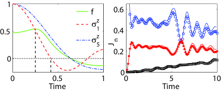
Figure 4: (Color online) Left panel: Evolution of the end- and central- spin polarizations and fidelity during the preparation of the end-polarized state. Chain length $N=9$, $\alpha=x,\bar{y}$, and $N_{\alpha}=2$. The two time points $t_{1}=0.25$ and $t_{1}^{\prime}=0.42$ are marked with vertical dashed lines. Right panel: MQC signal of $N=19$ spin chain with preparation time $t_{1}=0.25$. Intensities are normalized at every time as $J_{0}+2(J_{2}+J_{4})=1$. DQ Hamiltonian with NN+NNN couplings and the ideal end-polarized initial state – solid lines; DQ Hamiltonian with NN+NNN couplings and initial state synthesized at $t_{1}=0.25$ – circles for $J_{0}$, stars for $J_{2}$, and squares for $J_{4}$.

Starting from the two prepared states, $t_{1}=0.25$ and $t_{1}^{\prime}=0.42$, respectively, we calculate the MQC of the spin chain under the DQ Hamiltonian with NN+NNN couplings, and compare the results against those obtained for the ideal end-polarized initial state $\rho_{end}(0)$. The evolution of MQC for the initial state prepared with $t_{1}^{\prime}=0.42$ is quite different from that obtained with the intended state (data not shown), while the MQC of the initial state corresponding to preparation time $t_{1}=0.25$ is very close, as demonstrated in the right panel of Fig. 4. Note, however, that compared to the ideal end-polarized state, the experimentally prepared initial state shows slightly larger oscillations, especially in $J_{0}$.

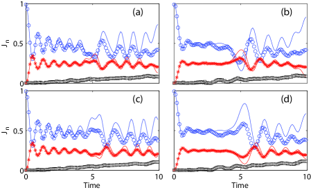
Figure 5: (Color online) Effect of NNN interactions in the DQ Hamiltonian for the thermal (left column – a and c) and the end-polarized initial state (right column – b and d). The length of the spin chain is $N=18$ (top row – a and b) and $19$ (bottom row – c and d). Solid (blue and red lines) are $J_{0}$ and $J_{2}$ computed from the analytical model, respectively. Circles, stars, and squares are $J_{0}$, $J_{2}$, and $J_{4}$ obtained from exact numerical results.

IV.2 Non-idealities in isolated single-chain dynamics

IV.2.1 Long-range couplings

As already remarked, appreciable growth of the four-quantum coherence signal at long times (Fig. 2) indicates the inadequacy of the analytical model, as the dynamics is no longer confined to a 1D system with pure NN couplings. Having shown in the previous section that the effect of higher-order AHT terms is negligible in the temporal region we consider, we next turn our attention to the influence of long-range couplings. We limit our calculations to the NNN couplings as they provide the most important correction to the analytical NN model.

Figure 5 shows the MQC signal obtained for spin chains of length $N=18$ (top) and $19$ (bottom) for the thermal state (left) and the end-polarized state (right), respectively. Both NN and NNN couplings in the DQ Hamiltonian are now exactly accounted for. By way of comparison, we also include the predictions from the analytical model. The following main observations may be made:

(i) NNN couplings produce even-order coherences greater than two, the largest contributions in the relevant time window arising from $J_{4}$. In general, even order coherences up to the number $N$ of spins in the chain may be expected. This is in contrast with the results based on a perturbative approach Feldman and Lacelle (1997), which yield MQC only up to the sixth order.

(ii) NNN couplings reduce the amplitude of the oscillations in $J_{0}$ and $J_{2}$.

(iii) The effect of NNN couplings is amplified at an instant in time that we call the mirror time, $t_{m}$ ($\approx 5$ in the figure), which is defined in terms of the analytical model as the time where $J_{0}$ shows a second largest oscillation for odd $N$ or the lowest point for even $N$. (Note that one could also equivalently define $t_{m}$ as the time where the second lowest/largest peak of $J_{2}$ occurs.) This effect is prominent in the numerical simulations, where one is necessarily constrained to relatively short chains. Qualitatively (see also Appendix B), the spin dynamics has a mirror symmetry about the middle spin, which causes the signal of specularly located spins to “interfere constructively” at the mirror time. This picture can also explain why the influence of NNN couplings on the dynamics of the chosen collective observable is most pronounced at this time: even small deviations from the ideal NN dynamics are able to destroy the interferences and can produce significant changes in the observed signal.

IV.2.2 Chain length distribution

Since the defects in the FAp sample are non-uniform, the spin chain length has a statistical distribution. According to the so-called random cluster model Cho and Yesinowski (1996), if defects are distributed randomly in the infinite 1D chain with a probability $(1-p)$, the average chain length is $\bar{N}=(1+p)/(1-p)$, and the relative fluctuation $\Delta N/\bar{N}=\sqrt{2p}\;/(1+p)$. For a low percentage of defects, ($p\approx 1$, $\bar{N}\gg 1$), the chain length distribution can be reasonably approximated by a uniform distribution of chain lengths. Fig. 6 shows the averaged MQC signal for an ensemble of chain lengths. Compared to an individual spin chain, the ensemble average washes out the long-time oscillations but leaves the short-time oscillations virtually unchanged. Since the concentration of defects is low in the actual sample, we expect that this effect will not be important on the time scales explored by the current experiments.

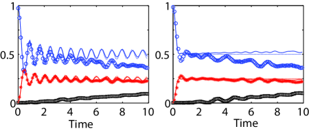
Figure 6: (Color online) Ensemble average of MQC signal for the thermal (left) and the end-polarized initial state (right), as resulting from a DQ Hamiltonian with NN and NNN couplings. Circles, stars, and squares show $J_{0}$, $J_{2}$ and $J_{4}$, respectively, with chain length averaged over $N=[17,21]$. For comparison, the solid lines are for a distribution of chains with average $\bar{N}=50$ in the random cluster model, evolved under the analytical model, whereas the dotted lines are for the zero and double quantum intensities for an infinite chain Feldman and Lacelle (1997).

IV.3 Non-idealities due to coupled-chain dynamics

Due to the 3D nature of the FAp sample, a given spin chain of interest (“central” spin chain henceforth) is coupled to all other chains in the crystal via the long-range dipolar coupling. Since the distance between two spin chains in FAp is about three times the distance of two NN ¹⁹F spins, the cross-chain couplings have about the same strength as the third-neighbor intra-chain coupling within a chain. The combined effect is, however, amplified by the presence of several (six) chains surrounding the central spin chain (recall Fig. 1). Furthermore, additional weaker contributions arise from more distant chains. Overall, the influence of the cross-chain coupling can thus be an important source of deviation from the analytical model, as we explore next.

Exactly modeling the influence of all chains on the central one would require us to simulate the quantum dynamics of a macroscopically large number of spins, which is clearly beyond reach. To make the problem numerically tractable, we thus need to reduce the many-body problem to a simpler model that represents as faithfully as possible those features of the real dynamics we are directly probing. In order to make sensible approximations, it is useful to reconsider the origin of the NMR signal in more detail. Let $M_{c}$ be the number of chains present in the crystal sample. In the high-temperature approximation, the initial density matrix of the whole system can be expressed as

$$\rho_{\text{3D}}(0)=\sum_{m=1}^{M_{c}}\rho_{m}(0),$$

where $m$ indexes the chains and $\rho_{m}(0)$ is either the thermal equilibrium state or the end-polarized state, as in Eqs. (4)-(5). Notice that due to its collective nature, the experimentally accessible observable can also be written as a sum of contributions from distinct chains. For the purpose of making contact with a reduced description where a single chain is singled out as a reference in the presence of other coupled chains, it is useful to view the total signal in the $k$-th measurement $S_{z}^{k}$ as originating from two terms, $S_{z}^{k}(t)=S_{z,intra}^{k}+S_{z,leak}^{k}$, with

$$S_{z,intra}^{k}(t)=\sum_{m=1}^{M_{c}}{\rm Tr}\Big{[}\sum_{j}\sigma_{mj}^{z}\rho_{m}^{k}(t)\Big{]},$$ (12a)

$$S_{z,leak}^{k}(t)=\sum_{m^{\prime}\neq m}{\rm Tr}\Big{[}\sum_{j}\sigma_{m^{\prime}j}^{z}\rho_{m}^{k}(t)\Big{]},$$ (12b)

where $\rho^{k}_{m}(t)=U_{k}(t)\rho_{m}(0)U_{k}^{\dagger}(t)$ (cf. Eq. (7)). These two terms reflect two different mechanisms by which the presence of cross-chain interactions can induce deviations of the experimental signal from that of an isolated chain.

The term in Eq. (12a), which we refer to as the intra-chain signal $S_{z,intra}^{k}(t)$, describes the signal obtained when the initial state and observable belong to the same chain: all other chains, which may initially be taken to be in the maximally mixed state, influence the reference chain in a “mean-field sense,” to the extent they modify $\rho^{k}_{m}(t)$. Were all the chains identical, the resulting signal would simply be $S_{z,intra}^{k}(t)\approx M_{c}{\rm Tr}[S_{z}\rho^{k}(t)]$, that is, an $M_{c}$-fold signal from a single chain coupled to the “environment chains”. Thus, $S_{z,intra}^{k}(t)$ may be well described within a “chain-plus-environment” model, where a single spin chain is coupled to a larger spin environment, and the measured NMR signal is determined completely by the reduced density matrix of the central chain – upon tracing over all environment spins, as in a standard formulation of the central-system-plus-bath problem CentrPlusBath ; FeynmanVernon ; SixManPaper .

While the intra-chain term describes a deviation from the ideal single-chain behavior that is not fundamentally different from, say, deviations induced by long-range couplings as analyzed in Sec. IV.2.1, the leakage signal $S_{z,leak}^{k}(t)$ in Eq. (12b) introduces a qualitatively different effect: that is, the possibility that some of the polarization initially located on the $m$th chain is transferred to the $m^{\prime}$th chains, and read out there. Since, from the point of view of the central spin chain, signal components would be ‘lost’ to the environment, a significant contribution $S_{z,leak}^{k}(t)$ would clearly indicate the inadequacy of a system-plus-environment picture at capturing the complexity of the underlying 3D strongly-correlated dynamics.

Even assuming that the consistency of a central chain-plus-environment treatment may be justified a posteriori by the smallness of the leakage signal for the evolution times of interest, modeling a realistic environment remains non-trivial because the actual crystal consists of a large number of quantum spin chains, evolving according to a highly complex, non-Markovian dynamics. In line with standard statistical approaches (including NMR relaxation theories) Kubo ; Slichter (1992), we can however reasonably argue that the main observed features should be robust with respect to the details of the environment description, as long as the relevant energy scales are correctly reproduced. In what follows, we will exemplify these considerations by separately investigating two models for describing how the coupling between different chains in FAp modifies the MQC dynamics of the central spin chain. In Sec. IV.3.1, a system of two coupled chains is investigated as a numerically accessible testbed where the ‘environment chain’ qualitatively retains the spatial structure of the FAp crystal. Physically, the latter feature is expected to be important (possibly essential) to properly represent the deviation induced in the idealized central-chain dynamics by the NN chains. In Sec. IV.3.2, a structureless spin environment model is considered instead, whereby the central chain couples to randomly placed spins. Physically, such a picture may be especially adequate to account for the net influence of distant chains. Computational constraints limit the size of the accessible model environment in both cases.

In spite of the above differences, it is important to realize that essentially the same type of simulations will be employed and the same main physics will be explored in both cases. In particular, the processes leading to deviations from the analytical model are primarily associated with the increased dimensionality of the Hilbert space and correlations between different chains in the sample. While no explicitly non-unitary evolution is present either in experiment or simulation, and the total system remains coherent at all times, a damping of the low-order MQC oscillations still emerges: as time progresses, a larger part of the Hilbert space is populated, and coherences of higher-order, which involve spins of different chains, build up at the expenses of low-order coherences. Relative to the observables that can be directly probed, the latter simply appear to unrecoverably decay.

IV.3.1 Effect of a structured spin environment

The correlated dynamics in nearby chains may be investigated by lumping together the contributions of the six nearest surrounding chains and treating them as a single chain, which couples coherently to the central spin chain, according to the DQ Hamiltonian. We take both chains to have length $N$ and start in the initial state of interest (either thermal or end-polarized). Since we are restricted to numerically calculate MQC for a system of up to $25$ spins, $N\lesssim 12$ in practice. Upon summation [$M_{c}=2$ in Eq. (12a)-(12b)], an upper bound to the NN cross-chain coupling strength is given by

$$\frac{\bar{b}_{\times}}{b}=\frac{\sum b_{\times}}{b} = -3\left(\frac{d}{D}\right)^{3}\approx-0.1488.$$ (13)

This approximation corresponds to neglecting correlations between spins from three or more different chains, which arise from higher-order cross-chain couplings in $S_{z,leak}^{k}(t)$ – for instance, the three-chain coupling is proportional to $(\bar{b}_{\times}/b)^{2}$. If such couplings are treated perturbatively, one may expect their effect to be negligible over the time scale of the experiment, as opposed to two-chain interactions which directly compete in strength with intra-chain NNN couplings. As discussed above, however, these two contributions may have very different physical implications, as the cross-chain coupling effect can genuinely increase the underlying Hilbert space, whereas NNN couplings can only increase the portion of the single spin-chain Hilbert space that is explored during the dynamics.

Exact calculation of the total signal $S_{z}^{k}(t)$ reveals that the contribution of cross-chain transfer due to $S_{z,leak}^{k}(t)$ remains small (below a few percents) over relatively short time scales (up to 5 in normalized units). As shown in Fig. 7, cross-chain couplings modeled in this way also damp the MQC oscillations at long times, similar to the effect of intra-chain NNN interations. Notice that at the mirror time, as observed in simulations with finite $N$, the effects of the cross-chain couplings are also amplified, further reducing the peak amplitude comment .

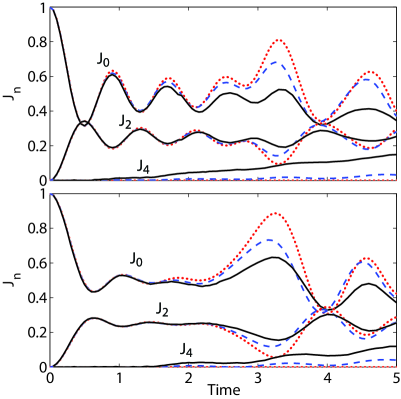
Figure 7: (Color online) Effect of cross-chain couplings for the thermal (top) and the end-polarized state (bottom). The length of each spin chain is $N=11$. Dotted lines represent the analytical isolated-chain NN prediction. Both NN and NNN couplings are considered in the exact simulation results for a single chain (dashed lines) as well as for two chains (solid lines) coupled according to Eq. (13).

IV.3.2 Effect of a structureless spin environment

According to our earlier discussion, another way to analyze the influence of cross-chain coupling that emphasizes the influence of far away chains is to consider an effectively structureless quantum spin environment BathRemark . In particular, the simplest choice is provided by a system consisting of spins arbitrarily (randomly) scattered in space. While of course nothing is arbitrary in the dynamics of the real FAp system, such a randomized model may just be viewed as a computationally accessible approximation of the complex dynamics under investigation.

Specifically, we reproduce the main features and the characteristic energy scales of the FAp sample driven by the $16$-pulse sequence by assuming that the $x$, $y$, $z$ coordinates of each of the 9 environment spins are drawn uniformly from $[-1,1]$. The $N=11$ spins of the central chain are placed equidistantly on the $z$-axis, with their $z$-coordinates also confined between $-1$ and $1$. The minimum distance between any pair of spins (whether environment or chain spins) is restricted to exceed 0.1 to prevent spins from being too close to each other. The central chain Hamiltonian of the form (1) is truncated at either the NN or NNN level (Fig. 8 and 9 respectively). All the dipolar coupling between the environment spins, and from the environment spins to the central spin chain are taken into account, as in Eq. (1), with the coupling constants $b_{j\ell}$ calculated from the spins coordinates. However, in order to have correct energy scales, all chain-environment coupling constants are rescaled to produce the correct value of the dispersion ${\rm Tr}\,[H^{2}_{CB}]$, where $H_{CB}$ is the chain-environment interaction Hamiltonian (see also Appendix D). This ensures that the couplings between the spins of different chains in FAp are $\approx 40$ times smaller than the couplings between the spins in the same chain. In a similar way, all couplings inside the environment are rescaled to produce a correct value for the Hamiltonian norms per spin, ${\rm Tr}\,[H^{2}_{C}]={\rm Tr}\,[H^{2}_{B}]$, where $H_{C}$, $H_{B}$ are the chain and environment Hamiltonians, respectively.

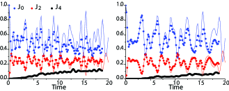
Figure 8: (Color online) $J_{0}(t)$, $J_{2}(t)$, and $J_{4}(t)$ for a chain of $N=11$ spins with thermal (left) and end-polarized (right) initial state. The chain is coupled to an environment of nine spins with random dipolar couplings. The lines are the analytical results for $J_{0}(t)$, $J_{2}(t)$. Note that only NN intra-chain couplings are included, however the times scales explored here are significantly longer than in any of the previous figures.

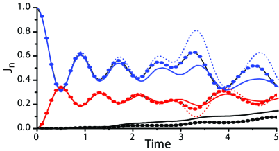
Figure 9: (Color online) Comparison between the effect of cross-chain couplings starting from the thermal state, as resulting from a structured two-chain system (solid lines) or from a coupling to a randomized spin (circles). In all cases, the length of the spin chain(s) is $N=11$ and NNN intra-chain couplings are included. Dotted lines represent the analytical prediction. Numerical results for $J_{0}(t)$ (blue), $J_{2}(t)$ (red), and $J_{4}(t)$ (black) MQCs are included.

We perform simulations of the total system treating it as a closed quantum system with unitary dynamics (see Appendix A for details). We simulate the evolution under the experimental DQ Hamiltonian, generated by the 16-pulse sequence. Each sequence with 16 pulses along the $x$-axis (preparation) and, afterward, the 16-pulse sequence with pulses along the $y$-axis is repeated five times (mixing). The pulses are ideal $\delta$-like, with varying inter-pulse separation, and the total time is varied from zero to 18.75 (in normalized units). Note that since the environment is homonuclear, it is affected by the pulses in the same way as the central chain. At the end of each protocol, the total NMR signal $S_{z}^{k}(t)$ is calculated by either (i) summing only the $z$-projections of the spins in the central chain, tracing out the environment spins (thus obtaining only the intra-chain contribution of Eq. (12a); or (ii) summing the $z$-projections of both the environment and the chain spins (thus also taking into account the leakage terms in Eq. (12b)). Comparison between the results (i) and (ii) shows that the leakage terms are small, on the order of about 1%. As in the two-chain model, we thus confirm a posteriori the validity of the underlying weak-coupling assumption between the central system and the rest.

Numerical results starting from the thermal and the end-polarized state are given in Fig. 8 for a single realization of such a random dipolarly-coupled environment, corresponding to a fixed (arbitrary) geometry of the spin lattice. While different realizations give very close results (data not shown), averaging over several realizations is impractical note . Fig. 8 also includes a comparison of the simulation results for $J_{0,2}(t)$ with the analytical model. The interaction with the environment leads to a significant damping of the oscillations of $J_{0}(t)$ and $J_{2}(t)$, and to an overall decay of these coherences. Interestingly, the decay of both $J_{0}(t)$ and $J_{2}(t)$ for the end-polarized initial state is slower than for the thermal initial state. Likewise, it is also worth noticing that the decay of the oscillations in $J_{2}$ is roughly a factor of two slower than the decay of $J_{0}$. This difference may be attributed to the fact that the random dipolarly-coupled environment is not fully structureless, as it possesses non-trivial integrals of motion (for instance the total magnetization of the central chain and the environment). The internal structure of the environment appears to strongly affect the dynamics of $J_{2}(t)$. This different behavior of the two MQC intensities is also present in the two coupled-chain simulations of Sec. IV.3.1, which are directly contrasted to the random spin-environment simulation results in Fig. 9. We further expand on these considerations by examining a chaotic spin bath model in Appendix C.

V Discussion and conclusion

We have investigated in detail the MQC dynamics of a quasi-1D spin chain in a fluorapatite crystal, both experimentally and numerically. By comparing exact simulation results with analytical solutions for the ideal DQ Hamiltonian with NN couplings, we have characterized the region of validity of this simple, single-chain NN model. For the initial states and observables of interest, we have found that for evolution times up to 0.5 ms (corresponding to about 5 times the inverse NN coupling strength) the system is experimentally indistinguishable from the single-chain, NN model. Simulations including long-range couplings within a single chain and across different chains reproduce well the experimental findings.

Beyond this time, the evolution deviates from the analytical model, although the deviations of the selected observables (the MQC) remain small. In principle, the experimental implementation of the DQ Hamiltonian using a simulation approach based on AHT is not a problem, at the evolution times considered. In addition, the dynamics of the experimentally created end-polarized initial state are seen to remain quite close to the dynamics of an ideal end-polarized state, as desired.

From simulations we observed that all the different types of long-range couplings analyzed lead to a qualitatively similar damping of the oscillations in the MQC signal and a relatively slow growth of the higher order coherences (in particular the 4-quantum coherence). In fact, a similar effect is also observed for a single chain coupled to a dipolar spin environment.

The similar behavior observed when introducing longer range couplings in a 1D chain and cross-chain couplings seems to indicate that although in the second case there are more pathways available for the propagation of multi-spin correlations, this effect cannot be observed in the MQC evolution. While it could be tempting to infer that the microscopic mechanisms leading to the observed behavior are to some extent similar in each case, it is also essential to acknowledge that the experimentally accessible, collective magnetization observable provides a highly coarse-grained visualization of the overall dynamics.

From a many-body physics standpoint, a deeper understanding of the influence of the structure of the longer-range dipolar couplings (“internal environment”) on MQC dynamics, in particular of the potentially higher level of sensitivity found for higher-coherence orders, is certainly very desirable.

Lastly, from a quantum communication perspective, our work calls attention to the added challenges that transport protocols need to face in the presence of limitations in available control, initialization, and readout capabilities, as well as long-range interactions and/or unwanted interactions with uncontrolled degrees of freedom. Our study points out that for the realization of precise transport, simply isolating a 1D system is not enough, as the deviation from an ideal NN model in a 1D chain caused by long-range couplings is as important as cross-chain couplings. Since a number of these issues are shared by all practical device technologies to a greater or lesser extent, it is our hope that our analysis will prompt further theoretical investigations of communication protocols under realistic operational and physical constraints.

Appendix A Numerical methods

We calibrate our numerical procedure by reproducing the results from the analytical model Cappellaro et al. (2007a, b). For sufficiently short spin chains, $N\leq 11$, we propagate exactly the density matrix of the system. That is, given an initial mixed state (either the thermal or the end-polarized state), we prepare the initial density matrix, evolve the system, obtain the density matrix at time $t$, and calculate the MQC signal according to Eq. (7). For longer spin chains, this approach becomes very inefficient due to the extremely high usage of computer memory (on the order of $4^{N}$ for a chain with $N$ spins). Instead, we employ a wave-function-based simulation method, whose memory usage scales as $2^{N}$.

To implement the wave-function simulation, we decompose the initial mixed density matrix of the system into a sum of $N$ (for the thermal state) or $2$ (for the end-polarized state) individual density matrices, and then approximate the $j$th density matrix with a product state of a known state of spin $j$ and a pure random state of the remaining spins Zhang et al. (2007, 2008). That is, we let

$$\sigma_{j}^{z}=\frac{1}{2}\Big{(}{\openone}_{j}-|\downarrow_{j}\rangle\langle\downarrow_{j}|\Big{)}\otimes|r_{j}\rangle\langle r_{j}|,$$

where $|r_{j}\rangle=\sum_{i=1}^{2^{N-1}}c_{i}|i\rangle$ is a linear combination of basis states of all spins except the $j$th spin, and $c_{i}$ is a random complex number obeying $\sum_{i=1}^{2^{N-1}}|c_{i}|^{2}=1$. Such a superposition is an exponentially accurate representation of the maximally mixed state, and in our simulations creates errors of about 0.5%. After preparing the initial wave-function, we propagate the system according to the Schrödinger equation, adopting an efficient algorithm based on Chebyshev polynomial expansion of the evolution operator Dobrovitski and De Raedt (2003).

In the calculation of the MQC signal for the system-plus-environment, an alternative way to prepare the initial state is used, by realizing that the initial density matrix may be expressed in terms of spin operators as follows. Let $|R\rangle=\sum_{i=1}^{2^{N}}c_{i}|i\rangle$ be a random wave-function of $N$ spins, and $|R^{\prime}\rangle=\sum_{j=1}^{N}\sigma_{j}^{z}|R\rangle$. Then we may simply write $\rho(0)=|R^{\prime}\rangle\langle R|$. The propagation of these two wave-functions is then implemented based on the methods mentioned above.

Appendix B Mirror Time

Besides the peak (dip) of the MQC signal and the amplification of the NNN coupling effects at the mirror time $t_{m}$, the following features may be interesting for spin transport in short spin chains:

(i) The mirror time increases linearly with the length of the spin chain $N$, as shown in Fig. 10(a).

(ii) For the same length spin chain, different locally polarized initial states have the same mirror time (of course, the thermal state, which may be seen as a mixture of different locally polarized initial states, also exhibits the same mirror time); See Fig. 10(b)-(c).

(iii) The NNN couplings shift the mirror time slightly.

These peculiar properties demand a better understanding of the physical meaning of the mirror time. In a picture of spin polarization transport along a chain Cappellaro et al. (2007b), starting from the end-polarized state where the polarization is pinned to spins $1$ and $N$, the polarization is transported to the central spin $(N-1)/2$ at the mirror time $t_{m}$ (we assume $N$ is odd for simplicity). As mentioned in the main text, the spin dynamics exhibits a mirror symmetry about the central spin, and thus interferes constructively at $t_{m}$. For other pairs of locally polarized initial states, for instance $\sigma_{j}^{z}$ and $\sigma_{N+1-j}^{z}$, the spin polarization also interferes constructively at the mirror time. The independence of $t_{m}$ on $j$ guarantees that the thermal state shows the same properties at $t_{m}$ as the end-polarized state.

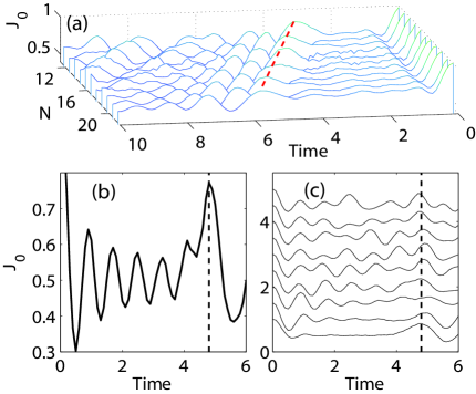
Figure 10: (Color online) (a) $J_{0}$ for the end-polarized initial state of different length spin chains (DQ Hamiltonian with NN+NNN couplings). The dashed line is a visual guide to the mirror time. (b) $J_{0}$ for the thermal initial state and (c) its partition for different locally polarized initial state $\sigma_{i}^{z}$ ($i=1,2,\cdots,9$). Due to the mirror symmetry of the chain, only half of the initial states are presented in panel (c). Each curve is shifted upward $0.5$ for a better view. The vertical dashed line specifies the position of mirror time $t_{m}$. For (b) and (c), the length of the spin chain is $N=17$.

Appendix C Chaotic Bath Model

Since in simulations we cannot exactly reproduce the many-body dynamics occurring in the FAp crystal, approximations are necessary at a number of levels. In representing the dynamics in terms of a single chain coupled to a bath the random dipolarly-coupled environment model used in the main text (Sec. IV.3.2) imposes a structure on the environment that is motivated by the physical system itself. From an open-system perspective, however, it may be interesting to explore alternative models for the bath, in order to have a sense of which details are important for the system’s dynamics and which are not. Although these alternative bath models need not have an immediate relevance to the experimental system, they may provide additional physical insight on the action of a spin bath in the FAp crystal. In this venue, it is useful to observe that quantum systems possessing a very complex behavior often exhibit similar features, and relevant aspects of their dynamics may be captured by quantum chaotic models, see e.g. Guhr98 . Following this approach, we emulate the bath’s internal dynamics using a chaotic spin-glass shard Hamiltonian gs ; jose . As a main feature, the chaotic bath model assumes that no integrals of motion exist for the bath other than the energy. This differs from the dipolarly-coupled environment model (and the real FAp sample), where the environment chains are similar to the central chain and, in the absence of pulses, the total magnetization of the central chain and the bath is conserved.

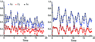
Figure 11: (Color online) $J_{0}(t)$, $J_{2}(t)$, and $J_{4}(t)$ for a chain with thermal initial state (left), and for the chain with end-polarized initial state (right). The chain is coupled to the bath of nine spins with chaotic glass-shard internal dynamics described by Eq. (14). Dash-dotted lines: Simulations with the dipolarly-coupled spin environment described in Sec. IV.3.2.

Specifically, in our case we choose the chain-bath coupling to mimic the arrangement of FAp samples: each chain spin is coupled to six bath spins, the coupling has a homonuclear secular dipolar form, similar to Eq. (1), and the coupling constants $b_{j\ell}$ for each pair of a chain and a bath spin are drawn uniformly from the interval $[-\sqrt{3}\cdot 0.025,\sqrt{3}\cdot 0.025]$. This ensures that the rms coupling between one bath spin and one chain spin is equal to the experimental value $b_{\times}/b\approx 0.025$, see Eq. (13). Nine bath spins are located on a $3\times 3$ square lattice, with a Hamiltonian

$$H_{B}=\sum_{\langle k,l\rangle}\Gamma_{kl}S^{x}_{k}S^{x}_{l}+\sum_{k}h^{z}_{k}S^{z}_{k}+\sum_{k}h^{x}_{k}S^{x}_{k},$$ (14)

where the summation in the first term is over NN pairs. The random couplings $\Gamma_{kl}$ and the local magnetic fields $h^{x,z}_{k}$ are drawn uniformly from the intervals $[-\Gamma_{0},\Gamma_{0}]$ and $[-h_{0},h_{0}]$, respectively, with the values of $\Gamma_{0}$ and $h_{0}$ adjusted to ensure: (i) chaotic regime, and (ii) correct characteristic energies for the spin dynamics inside the bath To achieve the latter, note that for a FAp chain with NN couplings only, and $N\gg 1$ spins, ${\rm Tr}{H^{2}}=(6/16)\ N\ {\rm Tr}{\openone}$, so that the rms energy per spin is 6/16. Correspondingly, the values of $\Gamma_{0}$ and $h_{0}$ were adjusted to give approximately the same rms energy per spin.

The results of the simulations for the thermal initial state and for the end-polarized initial state are given in Fig. 11. It is clearly seen that the interaction with the bath leads to significant damping of the oscillations of $J_{0}(t)$ and $J_{2}(t)$, and to an overall decay of these coherences, although the mirror time remains clearly visible. Interestingly, as also noted in the text, the decay of the zero- and second-order coherences $J_{0}(t)$ and $J_{2}(t)$ for the end-polarized state is slower than for thermal state. To further appreciate this, we compare the dynamics of $J_{0}(t)$ and $J_{2}(t)$ for the two bath models we examined in Fig. 11. The $J_{0}(t)$ signals for both bath models stay close to each other, while exhibiting significant damping of oscillations and overall decay in comparison with the analytical results for the isolated chain. In contrast, $J_{2}(t)$ for the random dipolarly-coupled environment stays rather close to the analytical prediction for the isolated chain, whereas $J_{2}(t)$ for the chaotic bath decays in the same way as $J_{0}(t)$ does. This suggests that the presence of extra integrals of motion does not significantly affect the dynamics of $J_{0}(t)$, whereas higher-order MQCs might more sensitively depend upon details of the open-system dynamics.

References

- (1)
- (2) D. D. Awschalom and M. E. Flatté, Nature Phys. 3, 153 (2007).
- Childress et al. (2006) L. Childress, M. V. G. Dutt, J. M. Taylor, A. S. Zibrov, F. Jelezko, J. Wrachtrup, P. R. Hemmer, and M. D. Lukin, Science 314, 281 (2006).
- (4) M. V. G. Dutt, L. Childress, J. Liang, E. Togan, J. Maze, F. Jelezko, A. S. Zibrov, P. Hemmer, and M. Lukin, Science 316, 1312 (2007).
- (5) F. H. L. Essler, H. Frahm, F. Gohmann, A. Klumper, V. E. Korepin, The one-dimensional Hubbard model (Cambridge University Press, 2005).
- Nielsen and Chuang (2000) M. A. Nielsen and I. L. Chuang, Quantum Computations and Quantum Information (Cambridge University Press, Cambridge, 2000).
- (7) S. Bose, Phys. Rev. Lett., 91, 207901 (2003).
- (8) S. Bose, eprint arXiv:quant-ph/0802.1224.
- (9) C. Di Franco, M. Paternostro, and M. S. Kim, eprint arXiv:quant-ph/0805.4365.
- (10) A. Kay, Phys. Rev. A 73, 032306 (2006).
- (11) M. Avellino, A. J. Fisher, and S. Bose, Phys. Rev. A 74, 012321 (2006).
- (12) G. Gualdi, V. Kostak, I. Marzoli, and P. Tombesi, Phys. Rev. A 78, 022325 (2008).
- (13) D. Burgarth, V. Giovannetti, and S. Bose, Phys. Rev. A 75, 062327 (2007).
- (14) J. Zhang, M. Ditty, D. Burgarth, C. A. Ryan, C. M. Chandrashekar, M. Laforest, O. Moussa, J. Baugh, and R. Laflamme, arXiv:quant-ph/0902.3719.
- (15) S. Lloyd, Science, 273, 1073 (1996).
- (16) I. Bloch, J. Dalibard, W. Zwerger, Rev. Mod. Phys., 80, 885 (2008).
- Cappellaro et al. (2007a) P. Cappellaro, C. Ramanathan, and D. G. Cory, Phys. Rev. A 76, 032317 (2007a).
- Cappellaro et al. (2007b) P. Cappellaro, C. Ramanathan, and D. G. Cory, Phys. Rev. Lett. 99, 250506 (2007b).
- (19) E. Rufeil-Fiori, C. M. Sanchez, F. Y. Oliva, H. M. Pastawski, P. R. Levstein, Phys. Rev. A 79, 032324 (2009).
- (20) M. Engelsberg, I. J. Lowe and J. L. Carolan, Phys. Rev. B 7, 924 (1973).
- (21) A. Sur and I. J. Lowe, Phys. Rev. B 12, 4597 (1975).
- (22) A. Sur, D. Jasnow and I. J. Lowe, Phys. Rev. B 12, 3845 (1975).
- (23) G. Cho and J. P. Yesinowski, Chem. Phys. Lett. 205, 1 (1993).
- Cho and Yesinowski (1996) G. Cho and J. P. Yesinowski, J. Phys. Chem. 100, 15716 (1996).
- (25) D. Stauffer and A. Aharony Introduction To Percolation Theory, CRC Press, 1994 pg 19-23
- Feldman and Lacelle (1997) E. Feldman and S. Lacelle, J. Chem. Phys. 107, 7067 (1997).
- (27) S. I. Doronin, I. I. Maksimov and E. B. Fel’dman, JETP 92, 597 (2000).
- (28) J. Fitzsimons and J. Twamley, Phys. Rev. Lett. 97, 090502 (pages 4) (2006).
- Slichter (1992) C. P. Slichter, Principles of Magnetic Resonance (Springer-Verlag, New York, 1992).
- Van Der Lugt and Caspers (1964) W. Van Der Lugt and W. J. Caspers, Physica 30, 1658 (1964).
- (31) N. Leroy, E. Bres, Eur. Cell. Mater. 2, 36 (2001).
- Xu et al. (2007) G. Xu, C. Broholm, Y.-A. Soh, G. Aeppli, J. F. DiTusa, Y. Chen, M. Kenzelmann, C. D. Frost, T. Ito, K. Oka, and H. Takagi, Science 317, 1049 (2007).
- (33) M. Munowitz and A. Pines, Adv. Chem. Phys., 66, 1-152 (1987).
- (34) H. Hatanaka, T. Terao, and T. Hashi, J. Phys. Soc. Japan 39, 835 (1975).
- (35) A. Pines, D. J. Ruben, S. Vega, and M. Mehring, Phys. Rev. Lett. 36, 110 (1976).
- (36) W. P. Aue, E. Batholdi, and R. R. Ernst, J. Chem. Phys. 64, 2229 (1976).
- (37) S. Vega, T. W. Shattuck, and A. Pines, Phys. Rev. Lett. 37, 43 (1976).
- (38) W. S. Warren, D. P. Weitekamp, and A. Pines, J. Chem. Phys. 73, 2084 (1980).
- (39) J. Baum, M. Munowitz, A. N. Garroway, and A. Pines, J. Chem. Phys. 83, 2015 (1985).
- (40) M. Munowitz, A. Pines, and M. Mehring, J. Chem. Phys. 86, 3172 (1987).
- (41) D. H. Levy and K. K. Gleason, J. Phys. Chem. 92, 8125 (1992).
- (42) S. Lacelle, S.-J. Hwang, and B. C. Gerstein, J. Chem. Phys. 99, 8407 (1993).
- Ramanathan et al. (2003) C. Ramanathan, H. Cho, P. Cappellaro, G. S. Boutis, and D. G. Cory, Chem. Phys. Lett. 369, 311 (2003).
- (44) H. J. Cho, T. D. Ladd, J. Baugh, D. G. Cory and C. Ramanathan, Phys. Rev. B 72, 054427 (2005).
- (45) H. J. Cho, P. Cappellaro, D. G. Cory and C. Ramanathan, Phys. Rev. B 74, 224434 (2006).
- (46) The relevant -pulse sequence S may be understood starting from a simpler -pulse cycle C which also simulates the DQ Hamiltonian, along with its time-reversed version . The primitive pulse cycle , where , being the pulse delay and the pulse width, respectively. Then Ramanathan et al. (2003).
- Haeberlen (1976) U. Haeberlen, High resolution NMR in solids: Selective averaging (Academic Press, New York, 1976).
- (48) W.-K. Rhim, A. Pines and J. S. Waugh, Phys. Rev. Lett. 25, 218 (1970).
- (49) H. G. Krojanski and D. Suter, Phys. Rev. Lett. 93, 090501 (2004).
- (50) Ph. Blanchard, D. Giulini, E. Joos, C. Kiefer, I.-O. Stamatescu (eds), Decoherence: Theoretical, Experimental and Conceptual Problems (Springer, Berlin, Heidelberg, New York, 2000).
- (51) R. P. Feynman and F. L. Vernon Jr., Ann. Phys. (NY) 24 118 (1963).
- (52) A. J. Leggett, S. Chakravarty, A. T. Dorsey, M. P. A. Fisher, A. Garg, and W. Zwerger, Rev. Mod. Phys. 59 1 (1995).
- (53) R. Kubo, M. Toda, and N. Hashitsume Statistical Physics II (Springer, New York, 1998).
- (54) As it turns out, the peak at the mirror time is no longer the second largest for the thermal state in the presence of cross-chain coupling, whereas it is still such for the end-polarized state.
- (55) It is worth noting that in some situations, the freedom of choice for the bath model can be formalized precisely: for instance, in the case of bosonic degrees of freedom, all baths possessing the same temperature and spectral density have, independently of any other detail, an equivalent effect on the central system, see e.g. FeynmanVernon ; SixManPaper . In the case of spin baths, as far as we know, such a degree of rigor has not yet been achieved.
- (56) A complete simulation for a fixed realization takes about a week on a -node cluster.
- Zhang et al. (2007) W. Zhang, N. P. Konstantinidis, K. A. Al-Hassanieh, and V. V. Dobrovitski, J. Phys.: Condens. Matter 19, 083202 (2007).
- Zhang et al. (2008) W. Zhang, N. P. Konstantinidis, V. V. Dobrovitski, B. N. Harmon, L. F. Santos, and L. Viola, Phys. Rev. B 77, 125336 (2008).
- Dobrovitski and De Raedt (2003) V. V. Dobrovitski and H. A. De Raedt, Phys. Rev. E 67, 056702 (2003).
- (60) T. Guhr, A. Müller-Groeling, H. A. Weidenmüller, Phys. Rep. 299, 189 (1998).
- (61) B. Georgeot and D. L. Shepelyansky, Phys. Rev. Lett. 81, 5129 (1998).
- (62) J. Lages, V. V. Dobrovitski, M. I. Katsnelson, H. A. De Raedt, and B. N. Harmon, Phys. Rev. E 72, 026225 (2005).