HISKP-TH-09/20, FZJ-IKP(TH)-2009-18
Non-perturbative methods for a chiral effective field
theory
of finite density nuclear systems
A. Lacoura, J. A. Ollerb, and U.-G. Meißnera,c
aHelmholtz-Institut für Strahlen- und Kernphysik (Theorie) and
Bethe Center for Theoretical Physics
Universität Bonn,
D-53115 Bonn, Germany
bDepartamento de Física, Universidad de Murcia, E-30071 Murcia,
Spain
cInstitut für Kernphysik, Institute for Advanced Simulation and
Jülich Center for Hadron Physics
Forschungszentrum Jülich, D-52425
Jülich,
Germany
Abstract
Recently we have developed a novel chiral power counting scheme for an effective field theory of nuclear matter with nucleons and pions as degrees of freedom [1]. It allows for a systematic expansion taking into account both local as well as pion-mediated multi-nucleon interactions. We apply this power counting in the present study to the evaluation of the pion self-energy and the energy density in nuclear and neutron matter at next-to-leading order. To implement this power counting in actual calculations we develop here a non-perturbative method based on Unitary Chiral Perturbation Theory for performing the required resummations. We show explicitly that the contributions to the pion self-energy with in-medium nucleon-nucleon interactions to this order cancel. The main trends for the energy density of symmetric nuclear and neutron matter are already reproduced at next-to-leading order. In addition, an accurate description of the neutron matter equation of state, as compared with sophisticated many-body calculations, is obtained by varying only slightly a subtraction constant around its expected value. The case of symmetric nuclear matter requires the introduction of an additional fine-tuned subtraction constant, parameterizing the effects from higher order contributions. With that, the empirical saturation point and the nuclear matter incompressiblity are well reproduced while the energy per nucleon as a function of density closely agrees with sophisticated calculations in the literature.
1 Introduction
In the last decades Effective Field Theory (EFT) has been applied to an increasingly wider range of phenomena, e.g. in condensed matter, nuclear and particle physics. An EFT is based on a power counting that establishes a hierarchy between the infinite amount of contributions. At a given order in the expansion only a finite amount of them has to be considered. The others are suppressed and constitute higher order contributions. In this work we employ Chiral Perturbation Theory (CHPT) [2, 3, 4], which is the low-energy EFT of QCD and takes pions (and nucleons as well for our present interests) as the degrees of freedom. CHPT is related to the underlying theory of strong interactions, QCD, because it shares the same symmetries, their breaking and low-energy spectrum. It has been successfully applied to the lightest nuclear systems of two, three and four nucleons [5, 6, 7, 8, 9, 10, 11]. Nonetheless, still some issues are raised concerning the full consistency of the approach and variations of the power counting have been suggested [12, 13, 14, 15, 16, 17, 18, 19]. A common technique for heavier nuclei is to employ the chiral nucleon-nucleon potential delivered by CHPT in standard many-body algorithms [20, 21], sometimes supplied with renormalization group techniques [22, 23]. One issue of foremost present interest is the role of multi-nucleon interactions involving three or more nucleons in nuclear matter and nuclei [24, 25, 20, 11, 23].
Ref. [26] derived many-body field theory from quantum field theory by considering nuclear matter as a continuous set of free nucleons at asymptotic times. The generating functional of CHPT in the presence of external sources was deduced, similarly as in the pion and pion-nucleon sectors [27, 28]. These results were applied in ref. [29] to study CHPT in nuclear matter, but including only nucleon interactions due to pion exchanges. Thus, the local nucleon-nucleon (and multi-nucleon) interactions were neglected. This approach was later extended in ref. [30] to finite nuclei and the pion-nucleus optical potential is calculated up to . In ref. [1] an extended power counting is derived that takes into account simultaneously short- and long-range multi-nucleon interactions. Notice that many present applications of CHPT to nuclei and nuclear matter [25, 31, 29, 32, 33, 34, 35, 36, 37, 38, 39] only consider meson-baryon Lagrangians. Short-range interactions are included without being fixed from the free nucleon-nucleon scattering. E.g. [35] fits the in-medium local nucleon-nucleon interaction, in terms of just one free parameter, to reproduce the saturation properties of symmetric nuclear matter. In addition, the nucleon propagators do not always count as , with a typical nucleon three-momentum, but often they do as the inverse of a nucleon kinetic energy, (with the nucleon mass), so that they are unnaturally large. This is well known since the seminal papers of Weinberg [3, 4]. This fact invalidates the straightforward application of the pion-nucleon power counting valid in vacuum as applied e.g. in refs. [29, 40, 31, 32, 33].
We implement here non-perturbative methods to perform actual calculations employing the power counting of ref. [1], which requires the resummation of some series of in-medium two-nucleon reducible diagrams. We employ the techniques of Unitary CHPT (UCHPT) [41, 42, 43, 44] that are extended to the nuclear medium systematically in a way consistent with the chiral power counting of ref. [1]. Our theory is applied to the problem of calculating up to next-to-leading order (NLO) the pion self-energy and energy density in asymmetric nuclear matter. The former problem is related to that of pionic atoms since the pion self-energy and the pion-nucleus optical potential are tightly connected [45, 46]. The issues of the pion-nucleus S-wave missing repulsion, the renormalization of the isovector scattering length in the medium [47, 37] and the energy dependence of the isovector amplitude [46] are not settled yet, despite the recent progresses [48, 46, 29]. Ref. [1] found that the leading corrections to the linear density approach for calculating the pion self-energy in nuclear matter are zero. We show here these cancellations explicitly within the developed non-perturbative techniques. We also show the related cancellation between some next-to-next-to-leading order (N2LO) pieces. The calculation of the energy density of nuclear matter starting from nuclear forces is a venerable problem in nuclear physics [49, 50, 51, 52, 53, 54, 31, 33, 35]. Our calculation of the energy density to NLO already leads to saturation for symmetric nuclear matter and repulsion for neutron matter. Indeed, an accurate reproduction of the equation of state for neutron matter can be achieved by varying slightly one subtraction constant around its expected value. For the case of symmetric nuclear matter an additional fine-tuning of a subtraction constant is necessary to obtain a remarkable good agreement between our results and previous existing sophisticated many-body calculations [49, 54, 55]. The saturation point and nuclear matter incompressibility are reproduced in good agreement with experiment.
After this introduction, we briefly review in section 2 the novel chiral power counting in the medium developed in ref. [1]. The contributions to the pion self-energy in the nuclear medium that arise from tree-level pion-nucleon scattering diagrams and from the one-pion loop nucleon self-energy are the subject of section 3. We dedicate section 5 to the evaluation of the part of the pion self-energy due to the dressing of the nucleon propagators in the medium because of the nucleon-nucleon interactions. For their calculation one requires the nucleon-nucleon scattering amplitudes in the nuclear medium which are calculated in the preceding section 4. The terms of the pion self-energy due to the nucleon-nucleon interactions that are not part of the nucleon self-energy are calculated in section 6 at NLO, where we also give some N2LO contributions. The derivation of the necessary loops involved in this calculation is performed in Appendix B. Section 7 is dedicated to the evaluation up to NLO of the energy density. Section 8 contains a short summary and the conclusions. In the Appendices we derive various results that are used in the main body of the paper. Appendix A offers a derivation of the partial wave expansion of nucleon-nucleon scattering in the nuclear medium and vacuum. The Appendices C, D and E develop the calculation of the in-medium integrals needed for the evaluations performed in other sections.
2 In-medium chiral power counting
We briefly review the chiral power counting for nuclear matter developed in ref. [1]. Let us start by introducing the concept of an “in-medium generalized vertex” (IGV) given in ref. [26]. Such type of vertices arises because one can connect several bilinear vacuum vertices through the exchange of baryon propagators with the flow through the loop of one unit of baryon number, contributed by the nucleon Fermi-seas. At least one Fermi-sea insertion is needed because otherwise we would have a closed vacuum nucleon loop that in a low-energy effective field theory is completely decoupled. It is also stressed in ref. [29] that within a nuclear environment a nucleon propagator could have a “standard” or “non-standard” chiral counting. To see this note that a soft momentum , related to pions or external sources can be associated to any of the vertices. Denoting by the on-shell four-momentum associated with one Fermi-sea insertion in the IGV, the four-momentum running through the nucleon propagator can be written as , so that
| (2.1) |
where , with the physical nucleon mass (not the bare one), and is the temporal component of . We have just shown in the previous equation the free part of an in-medium nucleon propagator because this is enough for our present discussion. Two different situations occur depending on the value of . If one has the standard counting so that the chiral expansion of the propagator in eq. (2.1) is
| (2.2) |
Thus, the baryon propagator counts as a quantity of . But it could also occur that is of the order of a kinetic nucleon energy in the nuclear medium or that it even vanishes.#1#1#1An explicit example is shown in section 6 of ref. [29] The dominant term in eq. (2.1) is then
| (2.3) |
and the nucleon propagator should be counted as , instead of the previous . This is referred to as the “non-standard” case in ref. [29]. We should stress that this situation also occurs already in the vacuum when considering the two-nucleon reducible diagrams in nucleon-nucleon scattering. This is indeed the reason advocated in ref. [3] for solving a Lippmann-Schwinger equation with the nucleon-nucleon potential given by the two-nucleon irreducible diagrams.
In order to treat chiral Lagrangians with an arbitrary number of baryon fields (bilinear, quartic, etc) ref. [1] considered firstly bilinear vertices like in refs. [26, 29], but now the additional exchanges of heavy meson fields of any type are allowed. The latter should be considered as merely auxiliary fields that allow one to find a tractable representation of the multi-nucleon interactions that result when the masses of the heavy mesons tend to infinity. Note that such methods are also used in the so-called nuclear lattice simulations, see e.g. [56]. These heavy meson fields are denoted in the following by , and a heavy meson propagator is counted as due to the large meson mass. On the other hand, ref. [1] takes the non-standard counting case from the start and any nucleon propagator is considered as . In this way, no diagram, whose chiral order is actually lower than expected if the nucleon propagators were counted assuming the standard rules, is lost. In the following are taken of the same chiral order, and are considered much smaller than a hadronic scale of several hundreds of MeV that results by integrating out all other particle types, including nucleons with larger three-momentum, heavy mesons and nucleon and delta resonances [4]. The formula obtained in ref. [1] for the chiral order of a given diagram is
| (2.4) |
where is the number of external pion lines, is the number of pion lines attached to a vertex without baryons, is the chiral order of the latter with its total number. In addition, is the chiral order of the vertex bilinear in the baryonic fields, is the number of mesonic lines attached to it, that of only the heavy lines, is the total number of bilinear vertices, is the number of IGVs and is the total number of baryon propagators minus , . The previous equation can be also written as
| (2.5) |
It is important to stress that is bounded from below as explicitly shown in ref. [1]. Because of the last term in eq. (2.4) adding a new IGV to a connected diagram increases the counting at least by one unit because . The number given in eq. (2.4) represents a lower bound for the actual chiral power of a diagram, , so that . The actual chiral order of a diagram might be higher than because the nucleon propagators are counted always as in eq. (2.4), while for some diagrams there could be propagators that follow the standard counting. Eq. (2.4) implies the following conditions for augmenting the number of lines in a diagram without increasing the chiral power by adding i) pionic lines attached to lowest order mesonic vertices, , ii) pionic lines attached to lowest order meson-baryon vertices, and iii) heavy mesonic lines attached to lowest order bilinear vertices, , . One major difference between our counting, eq. (2.5), and Weinberg one [3, 4] is that ours applies directly to the physical amplitudes while the latter applies only to the potential.
We apply eq. (2.4) by increasing step by step up to the order considered. For each then we look for those diagrams that do not further increase the order according to the rules i)–iii). Some of these diagrams are indeed of higher order and one can refrain from calculating them by establishing which of the nucleon propagators scale as . In this way, the actual chiral order of the diagrams is determined and one can select those diagrams that correspond to the precision required.
It is worth realizing that eq. (2.5) can be also applied in vacuum in order to determine the relative weight of the different diagrams. In this case, the needed Fermi-sea insertion for each IGV is split in two external nucleon lines, both in- and out-going ones. For vacuum is constant because in the EFT there is no explicit closed nucleon loops and baryon number is conserved. As stressed above, the expressions between brackets in eq. (2.5) do not increase despite the diagrams become increasingly complicated. As a result, one takes constant and determines the leading, next-to-leading, etc, contributions as indicated in the previous paragraph. In order to derive eq. (2.5) in ref. [1], a term was summed because for each IGV there is a Fermi-sea insertion. Since in vacuum there is no sum over nucleons in the sea, one should subtract this contribution so that we would have instead of . However, this just modifies the absolute order of a diagram but not the relative one between contributions which remains invariant, and this is what matters for explicit calculations.

3 Meson-baryon contributions to the pion self-energy
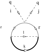
Here we start the application of the chiral counting in eq. (2.4) to calculate the pion self-energy in the nuclear medium up to NLO or . The different contributions are denoted by and are depicted in fig. 1. In terms of the pion self-energy the dressed pion propagators reads
| (3.1) |
The in-medium nucleon propagator [57], , is
| (3.2) |
In this equation the subscript refers to the third component of isospin of the nucleon, with for the proton and for the neutron, and is the corresponding Fermi momentum. We consider that isospin symmetry is conserved so that all the nucleon and pion masses are equal. The first term on the right hand side (r.h.s.) of the first line of eq. (3.2) is the so-called hole contribution and the last term is the particle part. In the second line, the first term is the free-space part of the in-medium nucleon propagator and the last term is the density-dependent one (or a Fermi-sea insertion). The proton and neutron propagators can be combined in a common expression
| (3.3) |
or in the equivalent form,
| (3.4) |
In the following, and correspond to the Pauli matrices in the spin and isospin spaces, respectively.
For the evaluation of the diagrams 1–6 we employ the and Heavy Baryon CHPT (HBCHPT) Lagrangians [58, 59]
| (3.5) |
where the ellipses represent terms that are not needed here. In this equation, is the two component field of the nucleons, is the axial-vector pion-nucleon coupling and the covariant chiral derivative, with . The pion fields enter in the matrix , in terms of which and , with the weak pion decay constant in the SU(2) chiral limit. The are chiral low-energy constants whose values are fitted from phenomenology [58]. The in-medium pion self-energy from in HBCHPT has been calculated up to two loops in refs. [60, 40].
The diagrams 1–6 were calculated in ref. [1]. We give here more details in their derivation. The first diagram in fig. 1 corresponds to
| (3.6) |
and arises by closing the Weinberg-Tomozawa term (WT) in pion-nucleon scattering. In the previous equation is the proton(neutron) density. is an S-wave isovector self-energy.
The diagram 2a in fig. 1 is represented by and is obtained by closing the nucleon pole terms in pion-nucleon scattering, with the one-pion vertex from the lowest order meson-baryon chiral Lagrangian [58],
| (3.7) |
In eq. (3.7) we have not included the in-medium part of the intermediate nucleon propagator because , so that the argument of the in-medium Dirac delta-function of eq. (3.4) cannot be fulfilled. By the same token
| (3.8) |
and the terms contribute one order higher than NLO. On the other hand,
| (3.9) |
and the term, when included in eq. (3.7), does not contribute because of the angular integration. Then,
| (3.10) |
The same procedure can be applied to the diagram 2b of fig. 1 (which corresponds to the same expression as but with the exchanges and ). Summing both, one has
| (3.11) |
The superscripts and refer to the isovector and isoscalar nature of the corresponding contribution to , respectively. Both are P-wave self-energies but is a recoil correction of and it is suppressed by the inverse of the nucleon mass.
The rest of the diagrams in fig. 1 are NLO. We now consider the sum of the diagrams 3a and 3b, where the squares indicate a NLO one-pion vertex from , eq. (3.5). It should be understood that the pion lines can leave or enter these diagrams. We also employ the expansion of eq. (3.8) for the nucleon propagator, although for this case it is only necessary to keep the term because the diagram is already a NLO contribution. The calculation yields
| (3.12) |
This is a P-wave isoscalar contribution. In this case the NLO pion-nucleon vertex is a recoil correction of the LO one and this is why is suppressed by the inverse of the nucleon mass. The diagram 4 in fig. 1 is given by
| (3.13) |
is an isoscalar contribution in which the term is P-wave and the rest is S-wave. Indeed, the low-energy constant is known to be dominated by the contribution of the [61]. For a Fermi momentum , corresponding to symmetric nuclear matter saturation, the Fermi energy of a two-nucleon system is around 80 MeV, which is still significantly smaller than the -nucleon mass difference. One then expects that integrating out the -resonance and parameterizing its effects in terms of the chiral counterterms is meaningful in the range of energies we are considering. This is indeed an important conclusion of ref. [62] where chiral EFTs with/without s are employed to evaluate different orders of the two-nucleon and three-nucleon potentials. We leave as a future improvement of our results to include explicitly the resonances.
Let us consider the contributions to the pion self-energy due to the one-pion loop nucleon self-energy. This is represented by the diagrams 5, 6a and 6b in fig. 1. These diagrams originate by dressing the in-medium nucleon propagator of the diagrams 1, 2a, 2b, in order, with the one-pion loop.

As a preliminary result let us first evaluate the nucleon self-energy in the nuclear medium corresponding to fig. 2. First, we consider the case of a neutral pion. The results for the charged pion contributions follow immediately from the case. In HBCHPT the proton self-energy due to the one- loop is given by,
| (3.14) |
Here, is the vector made up from the spatial components of and is the four-velocity normalized to unity (), such that the four-momentum of a nucleon is given by , with a small residual momentum (). In practical calculations we take and . Notice that the last integral in the previous equation is convergent because of the presence of the Dirac delta and Heaviside step functions. Instead of the full non-relativistic nucleon propagator eq (3.2), HBCHPT typically implies the so-called extreme non-relativistic limit in which , see e.g. ref. [58]. Given the properties of the covariant spin operator [58] it follows that
| (3.15) |
For the vacuum part we then have the integral,
| (3.16) |
This can be evaluated straightforwardly in dimensional regularization. Adding the contributions from the charged pions one has the free nucleon self-energy due to a one-pion loop [58], denoted in the following by ,
| (3.17) |
where and .#2#2#2In all the calculations that follow the square roots and logarithms have the cut along the negative real axis. In the previous expression we have subtracted the value of the one-pion loop nucleon self-energy at since we are using the physical nucleon mass. We also need below its derivative
| (3.18) |
The in-medium contribution to the proton self-energy due to the one- loop corresponds to the last line in eq. (3.14). Taking also into account the charged pions in the loop we have for the in-medium part of the one-pion loop contribution to the proton and neutron self-energies, and , respectively,
| (3.19) |
for our choice of and the second integral on the r.h.s. of eq. (3.14) reads
| (3.20) |
The step function in the previous integral implies the requirement . Then,
| (3.21) |
It is necessary that , otherwise would be larger than 1. This implies that
| (3.22) |
On the other hand, if then . Taking into account these constraints, one has:
| (3.23) |
The same expression of results for the cases a) and b),
| (3.24) |
In terms of the in-medium part of the one-pion loop contribution to the nucleon self-energy, eq. (3.19), reads
| (3.25) |
where the superscript refers to the pion species in the loop. The full in-medium nucleon self-energy is given by the sum of eqs. (3.17) and (3.25). In this way, the proton and neutron self-energies due to the one-pion loop are, in that order,
| (3.26) |
The self-energies for both the proton and neutron can be joined together in , given by
| (3.27) |
The diagram 5 of fig. 1 originates by dressing the in-medium nucleon propagator, eq. (3.4), with the in-medium one-pion loop nucleon self-energy. Its contribution, , can then be written as
| (3.28) |
with the convergence factor , , associated with any closed loop made up by a single nucleon line [57]. The trace acts in the spin and isospin spaces and gives the result
| (3.29) |
Next, we employ the identity
| (3.30) |
that follows from the r.h.s. of the first line of eq. (3.2). A similar identity also holds at the matrix level
| (3.31) |
because of the orthogonality of the isospin projectors and . Integrating by parts, as the convergence factor allows, we then have
| (3.32) |
We perform the integration over making use of the Cauchy-integration theorem. For that we close the integration contour along the upper -complex plane with an infinite semicircle. Because of the convergence factor the integration over the infinite semicircle is zero as along it. One should then study the positions of the poles and cuts in for and in eq. (3.32). First let us note that has only singularities for , as follows from eq. (3.16). This is also evident for the free part of , see eq. (3.2). As a result, there is no contribution when the integrand in eq. (3.32) involves only free nucleon propagators. The contribution with only the density-dependent part both in as well as in the nucleon propagator involved in the loop for is part of the diagram 7 in fig. 1, corresponding to a contribution. In fig. 3 we depict such an equivalence for the diagrams 5 and 7 of fig. 1. An analogous result would hold for the diagrams 6 and 8. The different contributions are evaluated in section 5, so we skip them right now.

Consequently we consider in this section only the contributions where we have simultaneously one free-space and one density-dependent part of the nucleon propagators involved in eq. (3.32) and in the calculation of . Two contributions arise. The first one results by employing the density-part for in the r.h.s. of eq. (3.2). The integration over is trivial due to the Dirac-delta function, with the result
| (3.33) |
We have introduced the shorter notation and .
The other contribution involves the free part of and can be written as
| (3.34) |
However, it is easily seen that this contribution, depicted in fig. 4, is indeed of . The reason is because there are two free nucleon propagators of standard counting (those with four-momentum in the figure, ), and each of them raises the counting with respect to given in eq. (2.5) by one power of the small scale. As a result, we neglect in the following . The same reasoning is not applicable for because only one nucleon propagator, the one inside the pion-loop self-energy, follows the standard counting. Nonetheless, the expression for , eq. (3.33), explicitly shows that it is actually a contribution of . This due to the fact that , as follows directly from eq. (3.18). We originally counted as because was taken as , since and . However, this evaluation of the order of a derivative, based on dimensional analysis, represents indeed a lower bound and its actual order might be higher, as it is the case here. This mismatch is due to the presence of the variable , defined after eq. (3.17), in addition to . The chiral order of the former is fixed by and not by . We also recall that there is another contribution to that results by keeping the density-dependent parts both in and , . It will be included in the evaluation of the contributions corresponding to the diagram 7 in fig. 1, section 5. is an isovector S-wave pion self-energy contribution.
We consider now the diagrams 6 of fig. 1. The diagram 6a gives
| (3.35) |
where we have omitted the Fermi-sea insertion in the intermediate propagator, following the discussion after eq. (3.7). is obtained from by replacing and in the latter. We now employ eq. (3.30), take into account that and integrate by parts in . In this way eq. (3.35) becomes
| (3.36) |
Following an analogous procedure for as the one given below eq. (3.32) for , the integration over is performed first. As a result, for the previous equation we only take the contributions that simultaneously involve one free-space and one density-dependent part of the nucleon propagators in and in the loop giving rise to . The contribution with only free-space parts vanishes because the integration over along the upper half-plane. While that with only density-dependent parts is included in the evaluation of the diagram 8 in fig. 1, section 5. On the other hand, applying here the argument in connection with fig. 4, the contribution involving the free-space parts of and the density-dependent one of in eq. (3.35) is because two free nucleon propagators (and not just one) are involved with standard counting. Hence, we neglect in the following this other contribution. In this way, we are left with the contribution, denoted by , that involves and the density-dependent parts in . From eq. (3.36) it is given by
| (3.37) |
Finally, taking into account the chiral expansion given in eq. (3.8) and adding , we have the new quantity given by
| (3.38) |
is a P-wave self-energy contribution. However, while the first term
on the r.h.s. is isovector, , the second term is
isoscalar, . It is also the case, see [1], that
is actually one order higher than expected, similarly as for
. For this follows obviously from its explicit
expression in eq. (3.38) as .
In this section we have undertaken the calculation of the diagrams in fig. 1 that can be fully accounted for by pion-nucleon dynamics. All the contributions calculated in this sections, to , as well as and , are linear in density. We have shown that to NLO only the leading contributions, and , and the NLO ones and have to be kept. and are finally one order higher.
4 Nucleon-nucleon interactions
The inclusion of the nucleon-nucleon interactions for the calculation of the pion self-energy takes place at NLO, because is required at least. As a result, it is necessary to work out the nucleon-nucleon interactions only at the lowest chiral order, . These contributions correspond to the diagrams 7–10 in the last two rows of fig. 1. First, we discuss these interactions in vacuum and then consider their extension to the nuclear medium. For the vacuum case we also discuss nucleon-nucleon scattering up to .
4.1 Free nucleon-nucleon interactions
The lowest order tree-level amplitudes for nucleon-nucleon scattering, ), are given by the one-pion exchange, with the lowest order pion-nucleon coupling, and local terms from the quartic nucleon Lagrangian without quark masses or derivatives
| (4.1) |
The fact that these are the leading tree-level contributions is a consequence of our counting eq. (2.5), which determines that the lowest order diagrams are those with and . The former arises from the contact interaction Lagrangian, eq. (4.1), and the latter corresponds to the lowest order one-pion exchange. The tree-level scattering amplitude for from eq. (4.1) is
| (4.2) |
where is a spin label and an isospin one. Obviously, this amplitude only contributes to the nucleon-nucleon S-waves. The one-pion exchange tree-level amplitude is
| (4.3) |
with and . The corresponding nucleon-nucleon partial waves due to one-pion exchange can be calculated using eq. (A.28). Instead, we first take the one-pion exchange between nucleon-nucleon states with definite spin and isospin, so that eq. (A.28) simplifies to
| (4.4) |
where and are the final and initial orbital angular momentum in the two-nucleon rest frame, respectively. Explicit expressions for are given in Appendix D of [63]. The sum of the local vertex, eq. (4.2), and the one-pion exchanges, eq. (4.3), is represented diagrammatically in the following by the exchange of a wiggly line, fig. 5.


Refs. [3, 4] argued that the two-nucleon reducible diagrams should be resummed because they are infrared enhanced (by large factors ) due to the large nucleon mass. This resummation, depicted in fig. 6, is required by our power counting, eq. (2.5), when the latter is applied to the vacuum case as discussed at the end of section 2. Notice that every two-nucleon reducible loop in the string is connected by adding local interactions and the exchange of pionic-lines at the lowest order. As pointed out in the conditions ii) and iii) of section 2 the counting does not increase then. Rephrasing the discussion of this section to the present case, the nucleon propagators in a two-nucleon reducible loop follow the non-standard counting and each of them is , so that altogether are . The leading wiggly line exchange is . When these two factors are multiplied by the contribution from the measure of the loop integrals, associated with the running momenta of the wiggly lines, an contribution results. The latter does not increase the chiral order and the series of diagrams in fig. 6 must be resummed.#3#3#3One could argue that if the nucleon propagator is taken as for the two-nucleon reducible loops, then the measure could be taken as , counting as . If this counting is followed, a suppression by an extra power of seems to arise. However, this factor is multiplied by the large nucleon mass, so that finally results, which is then multiplied by local interactions. If the latter count as , with , the resummation would be required as well within this point of view. We show below that this is the case in our approach. For this purpose, we follow the techniques of UCHPT [42, 44, 41] that performs this resummation partial wave by partial wave. Many recent nucleon-nucleon scattering analyses using CHPT [5, 6, 7, 8] follow refs. [3, 4] and solve the Lippmann-Schwinger equation in order to accomplish such resummation. UCHPT has been applied with great success in meson-meson [42, 64, 65] and meson-baryon scattering [66, 44, 67, 68, 69, 70].
The master equation for UCHPT is
| (4.5) |
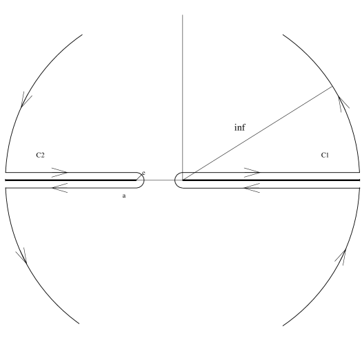
This equation, derived in detail in refs. [42, 44, 71], results by performing a once-subtracted dispersion relation of the inverse of a partial wave amplitude. The function is defined as follows. Let us denote by the center-of-mass (CM) three-momentum of the nucleon-nucleon system. A nucleon-nucleon partial wave amplitude has two cuts [72], the right hand-cut for , due to unitarity, and the left-hand cut for , due to the crossed channel dynamics. The upper limit for the latter interval is given by the one-pion exchange, as the pion is the lightest particle that can be exchanged. These cuts are represented in fig. 8. Because of unitarity, a partial wave satisfies in the CM frame that
| (4.6) |
above the elastic threshold and below the pion production one. The function in eq. (4.5) only has a right-hand cut and its discontinuity along this cut is times the right hand side of eq. (4.6). A once-subtracted dispersion relation can be written down given the degree of divergence of eq. (4.6) for . The integration contour taken is a circle of infinite radius centered at the origin that engulfs the right-hand cut, as shown in fig. 8 by . In this way
| (4.7) |
One subtraction has been taken at so that the integral is convergent. Note that the subtraction constant is the value of at , in particular, . Since , as discussed above, it follows that
| (4.8) |
The function corresponds to the divergent integral
| (4.9) |
The previous integral, depicted in fig. 7, is linearly divergent although it shares the same analytical properties as eq. (4.7). In dimensional regularization with one has, . This result is purely imaginary above threshold, , and it corresponds to the imaginary part of eq. (4.7). However, this is just a specific characteristic of the regularization method employed, since, as is explicitly shown in eq. (4.7), there is an undetermined constant . For the integral in eq. (4.9) is (infinitely-)negative, so that it is quite natural to assume that . Another more fundamental reason for taking , required by the consistency of the approach, is given below. In the following, we regularize any two-nucleon reducible loop in terms of the subtraction constant , taking into account eqs. (4.7) and (4.8). The irreducible diagrams with respect to intermediate multi-nucleon states will be regularized employing dimensional regularization [73]. This regularization method is shown up to NLO in the calculations performed in this work. For explicit calculations of loop integrals apart from within this scheme see Appendix D and the calculation of the energy per nucleon, in section 7.
Next, we consider how to fix in eq. (4.5). This function has only a left-hand cut, due to the exchange of pions in the chiral EFT (of course, in a meson-exchange calculation it would include further exchanges of other heavier mesons like , , etc). It has no right-hand cut since the latter is fully incorporated in the function by construction. As a result, should not be infrared enhanced since the effects of the large nucleon mass, associated with the two-nucleon reducible diagrams that give rise to the unitarity cut, are taken into account by eq. (4.5). Note that the latter results by integrating over the two-nucleon intermediate states at the level of the inverse of a partial wave, eq. (4.7). In a plain perturbative chiral calculation of a nucleon-nucleon partial wave the right-hand cut is not resummed and the convergence of the perturbative series is spoilt due to the infrared enhancement of the two-nucleon reducible loops. However, since the latter are resummed in eq. (4.5), the idea is to match this general equation with a perturbative calculation within CHPT up to the same number of two-nucleon reducible loops. The number must be the same to guarantee that is real along the physical region and fulfills the requirement of not having right-hand cut. We can make use of the geometric series in powers of of , eq. (4.5),
| (4.10) |
where we have used the matrix notation for the case with coupled channels. Here, just corresponds to the identity matrix times eq. (4.7), because the latter is the same for all partial waves. Together with the previous geometric series one also has the standard chiral expansion
| (4.11) |
with the chiral order indicated by the superscript. Now, for the determination of the different , , the matching between eq. (4.10) is performed with a perturbative chiral calculation for which the reducible part of every two-nucleon reducible (or unitarity) loop is counted as . It is important to stress that this counting is applied for calculating not , for the latter each two-nucleon reducible loop counts as , eq. (2.5). In this way, the matching up to a chiral order automatically comprises at most two-nucleon unitarity loops. In addition, the chiral order of the vertices employed will also make that no spurious imaginary parts are left since one is handling in the matching with perturbative unitarity up to order .
A few examples will clarify this process of matching and why it makes sense to take as the reducible part of a two-nucleon reducible loop for calculating within UCHPT. At lowest order, , there are no two-nucleon reducible loops and , where the latter is the tree-level calculation in CHPT at given by the sum of , eq. (4.2), and , eq. (4.3), projected in the appropriate partial wave. This is the wiggly line at the far left of fig. 6. At , , the only new contribution is the two-nucleon reducible part of the second diagram in fig. 6, denoted by for a given partial wave. Writing , and matching eq. (4.10) with the sum of the first two diagrams of fig. 6 one has
| (4.12) |
with the result
| (4.13) |
Notice that in the expansion of eq. (4.10) each factor of the kernel multiplies the loop function with its value on shell. This is why in eq. (4.12) we have for one iteration of , which is then subtracted from the function in eq. (4.13). This equation shows explicitly that the simultaneous expansion in chiral powers and number of loops for fixing implies that UCHPT really takes as the difference between a full calculation of one two-nucleon reducible loop and the result obtained by factorizing the vertices on-shell, eq. (4.10). Ultimately this relies on the fact that the difference has no right-hand cut, which is the one associated with the infrared enhanced two-nucleon reducible loops, and it has only left-hand cut. The latter is incorporated perturbatively in the interaction kernel , which is improved order by order. This is the reason why we have treated the expansion in two-nucleon reducible loops on the same foot as the chiral expansion. This procedure is iterated up to any desired order. E.g. at new contributions would arise that require the calculation of the irreducible part of the box diagram in fig. 6 and the reducible parts of the last diagram of fig. 6 with the wiggly line exchange iterated twice [74]. In addition, there are also local interaction terms from the quartic nucleon Lagrangian and two-nucleon irreducible pion loops [25, 8, 7, 73]. If we denote all these new contributions projected onto the corresponding partial wave by , the following equation results
| (4.14) |
The calculated up to some given order in the expansion eq. (4.11) is then substituted in eq. (4.5). On the other hand, one can match formally eq. (4.5) with a perturbative chiral calculation of for any value of the S-wave nucleon-nucleon scattering lengths because the latter enter parametrically in the calculation. This procedure gives rise to values of the low-energy constants and that are consistent with their ascribed scaling, see eq. (4.28) below. It is worth pointing out that eq. (4.5) is algebraic, so that the numerical burden for in-medium calculations is reduced tremendously.

The dependence on the parameter takes places because of the infrared enhanced two-nucleon reducible loops. This has made necessary to resum the right-hand cut, which requires the presence of one subtraction constant, , eq. (4.7). Indeed, for a fixed chiral order, according to the application of eq. (2.5) to nucleon-nucleon scattering in vacuum, the dependence on becomes smaller as higher powers of are considered for calculating , eq. (4.11). To show this, we need to take advantage of the analytical properties of , eq. (4.5). As discussed above, this quantity has only the left-hand cut, shown in fig. 8. For the following discussion we take the case of one uncoupled channel to simplify the writing. Its generalization to coupled channels is straightforward employing a matrix notation. The imaginary part of along the left-hand cut is given by,
| (4.15) |
Note that is real along the left-hand cut. We employ this result to write down a once-subtracted dispersion relation for . The integration contour is shown in fig. 8 as and consists of a circle of infinite radius centered at the origin that engulfs the left-hand cut.
| (4.16) |
We have taken one subtraction in the dispersion relation because the one-pion exchange amplitude, eq. (4.3), tends to a constant for . Then, we have for , eq. (4.5),
| (4.17) |
In order to solve eq. (4.16) one needs as input along the left-hand cut. CHPT could be used, since this imaginary part is due to multi-pion exchanges. As a result one could afford its calculation perturbatively because the infrared enhancements associated with the right-hand cut are absent in the discontinuity along the left-hand cut. The reason is because this discontinuity, according to Cutkosky’s theorem [75, 76], implies to put on-shell pionic lines so that within loops the pion poles are picked up making that the energy along nucleon propagators now is of , instead of a nucleon kinetic energy. In this way, the order of the diagram rises compared to that of the reducible parts and it becomes a perturbation. E.g., let us take as illustration the last diagram on the r.h.s. of fig. 9, corresponding to the twice iterated one-pion exchange. Its reducible part is infrared enhanced, which has been calculated by us in the presence of the nuclear medium, in agreement with ref. [59] when reduced to the vacuum case. However, its discontinuity across the left-hand cut arises by putting on-shell the two intermediate pion lines. Its leading contribution to in a expansion in the -channel CM frame is given by
| (4.18) |
with and is a numerical factor due to the spin algebra. No factor appears in the numerator and it follows the standard chiral counting. In this way, the leading contribution to along the left-hand cut is given by the one-pion exchange. The latter can then be inserted in eq. (4.16), once projected in a given partial wave. The solution of this equation would correspond to the leading result for in the chiral expansion of eq. (2.5), without involving the expansion in the number of two-nucleon reducible loops. This interesting exercise will be left for future consideration.
Pion exchange amplitudes are treated perturbatively in the Kaplan-Savage-Wise (KSW) power counting [12, 13]. This is done for any energy region and, in particular, along both the right- and left-hand cuts. On the other hand, the dispersive treatment offered here only needs as input the discontinuity (imaginary part) of a nucleon-nucleon partial wave along the left-hand cut, see eq. (4.17). This discontinuity arises due to pion exchanges which, as discussed in the previous paragraph, could be calculated perturbatively in CHPT. Differences with respect to KSW arise due to the resummation of the right-hand-cut in eq. (4.17), including both local and pion-exchange contributions. This would correspond to higher orders in KSW power counting [13]. Notice also that while KSW is a strict perturbation theory calculation in quantum field theory (QFT) ours merges inputs from perturbative QFT and S-matrix theory, see e.g. ref. [77] for a pedagogical account of first applications of the similar N/D method to nucleon-nucleon scattering.
Two subtraction constants appear in eq. (4.17), from eq. (4.16) and from the function , eq. (4.7). We are going to show that they are not independent, however. The two constants have appeared due to the splitting between the functions and when expressing , eq. (4.5). This is analogous to the standard fact that in any renormalization scheme there is an exchange of contributions between local parts in loops and local counterterms. In order to proceed with the demonstration that the resulting , eq. (4.17), does not depend on the subtraction constant , let us write directly a dispersion relation for taking the contour in fig. 8
| (4.19) |
where . The last term in the previous equation gives contribution for and arises due to the behaviour at threshold of a partial wave, vanishing as . Two-body unitarity is assumed all the way along the right-hand cut in the first integral. This is not essential for the discussion that follows and we could have written directly Im along the right-hand cut, as done for the left-hand one.#4#4#4 In eq. (4.19) we could use different subtraction points for the two integrals, e.g. and , respectively. One then has (4.20) As discussed above the input for solving in eq. (4.16) is along the left-hand cut. This can also be shown explicitly from eq. (4.19) by writing , as follows from eq. (4.5). Subtracting from we arrive to the following equation for ,
| (4.21) |
In the following we omit the last term in the previous equation for simplicity, since it does not depend on . The reader could include it straightforwardly if desired. If eq. (4.21) is solved by iteration, it is straightforward to show that does not depend on at any order in the iteration. The zeroth iterated solution is , which yields . Obviously, the sum is independent of . For the first iterated solution one has
| (4.22) |
Notice that only the combination appears in the integral, which is independent of . However, depends explicitly on due to the term before the integral. Nevertheless, given that , the first on the r.h.s. of eq. (4.22) is accompanied again with so that no dependence on is left. This process can be straightforwardly generalized to any order. For the iteration the combination that appears in before the integral is added to for calculating , so that no dependence on arises from this fact. In addition, under the integration sign we have repeatedly times the same term , which does not depend on .
From the previous discussion, one concludes quite confidently that no -dependence is left because this was the case for evaluated at any order in the iterative solution of , eq. (4.21). In this way, it is clear that one could interpret the constant , eq. (4.7), and the subtraction point in close analogy with renormalization theory. The latter corresponds to the “renormalization scale” and the former fixes the “renormalization scheme”. For a given then is fixed so as to reproduce at the point . The dependence on is then transmuted into the experimental input . The final result should be independent of , which in turn, by taking the derivative of , eq. (4.17), with respect to this parameter implies the equation
| (4.23) |
This discussion also shows that one always has the freedom to take to be the same for all the partial waves, as we have done.#5#5#5There is an infinity of solutions of eq. (4.19) differing between each other in the number of zeros of . Each of these zeros is a pole of so that it brings altogether as free parameters the position of the pole and its residue. They are the so-called Castillejo-Dalitz-Dyson (CDD) poles [78]. The CDD poles are typically associated with resonances [79, 78]. Notice that a pole in typically makes its real part to vanish if the remnant is a smooth function of energy around the pole. In low energy S-wave meson-meson scattering the Adler zeros correspond to CDD poles [42]. However, for nucleon-nucleon scattering there is no evidence for a low energy zero in the partial waves (apart from the trivial one at threshold for .) In the pionless EFT for nucleon-nucleon interactions the third integration on the r.h.s. of eq. (4.19) is absent. The infinity tower of chiral counterterms in this EFT can be accounted for by adding CDD poles, see ref. [42] where this is shown explicitly for a similar problem.
For higher partial waves it is convenient to derive the dispersion relation for instead of eq. (4.17). In this way, the low energy behaviour of a partial wave as for is ensured, independently of the approximation for [80]. The resulting expression is
| (4.24) |
Note also that for no subtraction is needed if (mod ) for , as in the one-pion exchange. Then, one could also rewrite the previous equation for as
| (4.25) |
The degree of divergence of for increases by including higher order loop contributions, see e.g. eq. (4.18). As a result, more subtractions should be taken and the resulting subtraction constants could be related with higher order chiral counterterms.
We have proposed to consider as in order to fix . Indeed, is suppressed along the left-hand cut, vanishing in the low momentum region of the dispersive integral of eq. (4.16), which dominates its final value for low energy nucleon-nucleon scattering. On the physical Riemann sheet , with , and since is negative and of natural size , it tends to cancel with and becomes zero for . This is an important reason for having taken above. Proceeding along these lines, so that is treated as relatively small along the left-hand cut, eq. (4.16) would simplify at leading order. On the one hand, is replaced by 1 and, on the other, is given by the one-pion exchange. Hence, one obtains for in S-wave the sum of a constant plus one-pion exchange (resulting from the dispersive integral), precisely the content of the wiggly lines, fig. 5. For let us take directly eq. (4.25). In this way, when neglecting , the dispersive integral just gives rise to the one-pion exchange, as was the case for our previously calculated . One could continue further in this way, and solve eq. (4.16) in a power series expansion of along the left-hand cut at each chiral order in the calculation of . The truncation of such expansion leaves a residual dependence. We have followed the same point of view in order to determine through the matching process discussed above. Indeed, alternatively to performing the geometric series expansion of eq. (4.10), we could consider directly the inverse of , similarly as done in order to obtain eq. (4.15). Then, it follows from eq. (4.5) that
| (4.26) |
The first method discussed above for determining is the perturbative solution of eq. (4.26) in a chiral series of powers of . The solutions of eqs. (4.26) and (4.16) employing the perturbative method are equivalent because from eq. (4.26) has only a left-hand cut, being its imaginary part along this cut the same as eq. (4.15), and it is analytical, so that it satisfies the perturbative version in power of of the dispersion relation eq. (4.16).#6#6#6We have shown this equivalence explicitly for . It is also straightforward to show it for . The following remark is in order. The perturbative solution in the chiral expansion of powers of of eq. (4.26) has the advantages over solving eq. (4.16) that it is algebraic and the chiral counterterms in are taken into account in the solution in a straightforward manner. It is also very versatile, so that it can be extrapolated straightforwardly to correct by initial and final state interactions and to the nuclear medium. Notice that eq. (4.26) can only be solved perturbatively since the input is calculated in CHPT and only fulfills unitarity perturbatively. However, the exact solution of the integral equation eq. (4.16) has the advantage of not requiring the expansion in powers of but just the chiral series on along the left-hand cut, and the latter expansion rests in a sound basis as discussed above.
We now concentrate on fixing the constants and from the local quartic nucleon Lagrangian, eq. (4.1). These constants and , eq. (4.8), are the only free parameters that enter in the evaluation of the nucleon-nucleon scattering amplitudes from eq. (4.5) up to . We first discuss the LO result and then the NLO one. and are fixed by considering the S-wave nucleon-nucleon scattering lengths and for the triplet and singlet channels, respectively. At we have at threshold
| (4.27) |
The triplet S-wave is elastic at this energy, without mixing with the partial wave, because of the vanishing of the three-momentum. The resulting expressions for the scattering lengths from eq. (4.27) imply that
| (4.28) |
One of the benchmark characteristics of nucleon-nucleon scattering are the large absolute values of the S-wave scattering lengths fm and fm, so that , . Given the expression for the imaginary part of above threshold in eq. (4.7) one can estimate that ,#7#7#7As explicitly shown in the second line of eq. (4.7) one can trade between the subtraction constant and just by changing the subtraction point. In a natural way, both should be taken of similar size for estimations. which is then much larger in absolute value than and , although there is a difference because is smaller by around a factor 4 than . As a result, it follows from eq. (4.28) that . In this way, the low-energy constants and do not diverge for , and after iteration it is still consistent to treat , eq. (4.1), as . Notice as well that the one loop iteration of the contact terms compared in absolute value with the tree level goes like , taking into account the expression for given in eq. (4.7). The three-momentum is divided by the scale , considering the just given estimates for and . This justifies to iterate these diagrams for as discussed above. For the case of the once-iterated pion exchange one would have the factor as compared with the tree level one-pion exchange. Then is divided by the scale , and the one-pion exchange should be as well iterated together with the lowest order contact terms. The issue of iterating potential pions is analyzed in detail in ref. [13], in order to understand the failure of the KSW power counting in some triplet channels, particularly, for the and channels. The authors of ref. [13] conclude that for some spin triplet channels the summation of potential pion diagrams is necessary to reproduce observables, while for the singlet channels this iteration does not seem to be a significant improvement over treating pion exchanges perturbatively.
Only local terms and one-pion exchange contributions enter in the calculation of . This is rather simplistic in order to describe properly the nucleon-nucleon interactions as a function of energy soon above threshold. Let us now consider eq. (4.5) with up to . At this order, along the left-hand cut is still given by the one-pion exchange, so that the exact solution of eq. (4.16) for would be the same. The differences observed in the results at and are then due to keep a one more factor in the perturbative solution of eq. (4.16). This discussion shows clearly the mixed nature of the chiral expansion in powers of for obtaining .
We employ the and scattering lengths for evaluating and at . We denote by any of these scattering lengths and apply eq. (4.5) at threshold. We obtain
| (4.29) |
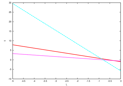
Taking eq. (4.13) at threshold we rewrite and express because the box diagram , fig. 9, consists of four contributions with two, one and zero local vertices. The first contribution is given by , the second by and the last one by , respectively. The coefficients and are given in terms of and the known parameters , and . is the same for the partial waves and while is different. The values of and as a function of are shown in fig. 10. Substituting these expressions in eq. (4.29)
| (4.30) |
with the result.
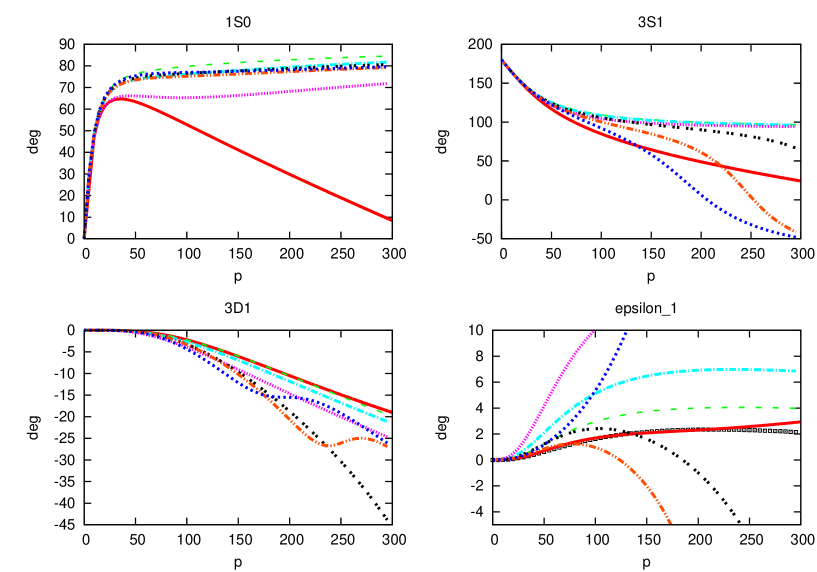
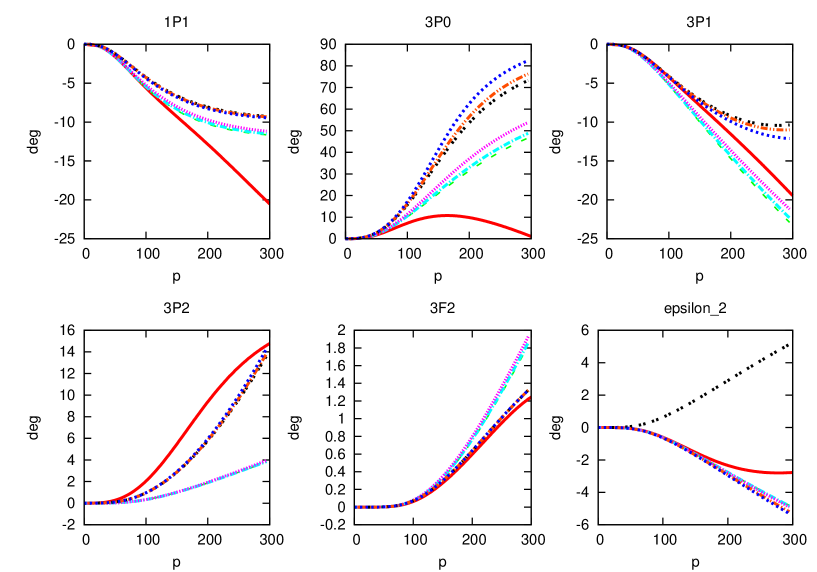
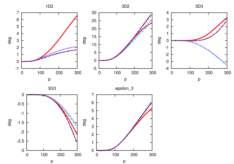
In figs. 11, 12 and 13 we show the LO and NLO results for the nucleon-nucleon scattering data (phase shifts and mixing angles) up to MeV making use of eq. (4.5). Since at LO is close to , as explained above, we show the results for the values , and because its inverses are , and , respectively. In this way, the resulting at LO is of order , a natural size. E.g. employing the estimation for , given below eq. (4.28), one would obtain . On the other hand, let us recall that negative values for , and not far from , are the required ones in order to optimize the perturbative solution of eq. (4.16). For the LO results the lines are the dashed, dot-dashed and dotted lines, corresponding to , and , respectively. While to NLO these are the double-dotted, double-dot-dashed and short-dashed lines, in the same order. For MeV the pion production threshold opens and it does not make sense to compare with data above this point. An calculation, which includes important new physical mechanisms, as non-reducible two-pion exchanges between others, as indicated above before eq. (4.14), is presumably needed to improve the agreement with data [5, 8]. E.g., it is well known that for the partial wave an chiral counterterm, in the standard chiral counting,#8#8#8At in the KSW counting [12]. is required in order to reproduce its relatively large effective range so that the agreement with data improves. This can be understood by considering the effective range expansion. For the partial wave is extremely small so that the contribution from the effective range rapidly overcomes (the leading order contribution). Then, this problem is not so much related to the fact of having too large higher order corrections but more it arises because the leading order is anomalously small. The largest differences in absolute values between the LO and NLO results are observed in the - and partial waves. These partial waves, as discussed in depth in ref.[13], have large non-analytic corrections from two potential pion exchange. For the , and waves the difference in absolute terms is small, a few degrees, although relatively it can be large typically for MeV. For higher partial waves these differences are typically much smaller since the iteration of one-pion exchange becomes smaller [59]. Our results are of comparable quality to those obtained at LO within the Weinberg’s counting approach [8]. The phase shifts are also not well reproduced at this order in ref. [8]. Both approaches share the same input for along the left-hand cut, and at we have already considered the iteration of one factor in determining , as discussed above. The main differences between our results and ref. [8] at LO concern and the phase shifts for and . For the latter our results are closer to experiment while for the two former observables the LO calculation of ref. [8] is closer to data. It is known that one-pion exchange has a too large tensor force which is reduced by higher order counterterms. In the meson exchange picture this cancellation at short distances of the one-pion exchange tensor force is produced by the exchange of -mesons [83]. The mixing - and the partial wave have large attractive matrix elements of the one-pion exchange tensor operator, as stressed in refs. [15, 21]. These are the partial waves that depart more from data in absolute terms. The phase shifts were reproduced accurately in ref. [15] at LO for low energies. In this reference, a counterterm was promoted to LO in all the partial waves with attractive tensor interactions, and in particular to the channel. Such free parameter is needed to fit the data [15, 8]. The results of ref. [15] are then cut-off independent for high enough values of the employed cut-off.
As a result of the perturbative approach actually followed in this paper for determining by solving eq. (4.26) in an expansion in the number of two-nucleon reducible loops, a residual dependence on is left in the solution due to higher orders in this expansion (and not from the pure chiral one, eq. (2.5)). As more orders are included the exact solution of , obtained by solving eq. (4.16), is better approached and any dependence on should tend to vanish. From here one could also infer that contributions with one-pion exchange twice iterated in are expected to be significant at least in those observables with a clear dependence in figs. 11-13. It is also worth noticing that the dependence on in figs. 11-13 at LO/NLO is much smaller for the P- and higher partial waves than for the S-waves. This should be expected because for vanishes at threshold as so that both and are small in the low energy part of the left-hand cut. In this way the perturbative solution of eq. (4.16) should typically converge faster for higher . Conversely, the convergence of the S-waves should be slower, something that it is clear for the coupled channels from fig. 11. Particularly noticeable is the dependence on of , a fact that is in agreement with the results of Fleming, Mehen and Stewart [13]. The squared points in the panel for in fig. 11 are obtained with . They agree closely with data [81], though such good agreement seems to be accidental.
4.2 Nucleon-nucleon scattering in the nuclear medium
When calculating a loop function in the nuclear medium we typically use the notation , where indicates the number of two-nucleon states in the diagram (0 or 1) and the number of pion exchanges (0, 1 or 2). In addition, we also use , and , with the subscripts , and indicating zero, one or two Fermi-sea insertions from the nucleon propagators in the medium, respectively. In this way, the function and its in-medium counterpart is , that is calculated in the Appendix C.
The evaluation of the nucleon-nucleon scattering amplitudes in the nuclear medium at lowest order can be easily obtained from our previous result in vacuum since the only modification without increasing the chiral order corresponds to use the full in-medium nucleon propagators. This is directly accomplished by replacing by in eq. (4.5). At any order for nucleon-nucleon scattering in the nuclear medium, we use eq. (4.5) but now with the function substituted by so that
| (4.31) |
The same process as previously discussed is followed to fix . Note
that any other in-medium contribution requires , which then
increases the order at least by one more unit, cf. eq. (2.4). This new
in-medium generalized vertex must be associated with the nucleon-nucleon
scattering diagrams of leading order. The modification of the meson
propagators (both heavy and pionic ones) by the inclusion of an in-medium
generalized vertex increases the chiral order by two units. However, the
modification of the enhanced nucleon propagators with one in-medium
generalized vertex only increases the order by one unit and these
contributions must be kept at NLO. It goes beyond the scope of this article
to offer a complete study of the in-medium pion self-energy at N2LO where
the full NLO in-medium nucleon-nucleon interactions are needed. What we do
here for illustration is to change the free nucleon propagators by the
in-medium ones in the calculation of the box diagram that enter
in fixing , eq. (4.13), with also replaced by
.
In eq. (4.31) we have included the superscript , which
corresponds to the third component of the total isospin of the two nucleons
involved in the scattering process, both in the partial wave
and in , as the Fermi momentum
of the neutrons and protons are different for asymmetric nuclear matter.
The function conserves total isospin , because it is
symmetric under the exchange of the two nucleons, though it depends on the
charge (or third component of the total isospin) of the intermediate state.
This is a general rule, all the operators are symmetric under the
exchange , so that they do not mix isospin representations
with different exchange symmetry properties.
In this section we have determined the vacuum nucleon-nucleon scattering at LO and NLO
following the novel counting of eq. (2.5) [1]. For nuclear matter the LO
nucleon-nucleon scattering amplitudes have been also obtained. The infrared enhancement of the two-nucleon reducible
loops have made it necessary to resum the right-hand cut. This is accomplished by
a once-subtracted dispersion relation of the inverse of a partial wave giving rise to eq. (4.5).
The important function , eq. (4.7), which is defined in terms of a subtraction constant, or , is introduced.
It has been argued that the subtraction constant is , because by changing the
subtraction point the subtraction constant is modified reshuffling the form of the function , which is invariant. The process for determining the interaction kernel , eq. (4.5),
has been
also discussed in detail. It was obtained that the subtraction point acts as a “renormalization scale” where an experimental point is reproduced. The subtraction constant just fixes the “renormalization scheme” and the exact results should not depend on it. A natural value for was argued to be adequate for obtaining as a perturbative solution of eq. (4.16) in order to suppress the effects of the iterative factor in the equation. The couplings and from the local nucleon-nucleon Lagrangian, eq. (4.1), have been fixed in terms of at LO and NLO reproducing the S-wave nucleon-nucleon scattering lengths. These couplings keep their estimated size
of after the iteration, despite the well known fact that the nucleon-nucleon scattering lengths are much larger than . The resulting phase shifts and mixing angles at LO and NLO are depicted in figs. 11, 12 and 13. It is argued that higher orders should be included in order to improve the reproduction of data. Particularly, a N2LO analysis should be pursued since it would include the important two-pion irreducible exchange and new counterterms, in particular the one necessary to reproduce the effective range for the partial wave [11]. This is left as a future task since our present main aim is to work the results up to NLO and settle the formalism in detail.
5 Contributions from the nucleon self-energy due to nuclear interactions
In this section we consider those diagrams in fig. 1 that include the nucleon-nucleon contributions to the nucleon self-energy in the medium, diagrams 7 and 8. In turn, for each of these figures the one on the top corresponds to the direct nucleon-nucleon interactions, while the exchange part gives rise to the diagram on the bottom (that includes the part of the diagrams 5 and 6 with all nucleon propagators corresponding to Fermi-sea insertions.)
First, let us consider the evaluation of the diagrams 7 in fig. 1, denoted by . It is given by
| (5.1) |
where
| (5.2) |
with and the proton and neutron self-energies due to the nucleon-nucleon interactions, in order. Performing the trace in isospin,
| (5.3) |
Here corresponds to the spin of the incident nucleon. Taking into account the identity eq. (3.30) we can integrate by parts eq. (5.3) with the result
| (5.4) |

The nucleon self-energy due to the nucleon-nucleon interactions, represented in fig. 14, is given by the expression
| (5.5) |
where is the two-nucleon scattering operator between the nucleon states characterized by the four-momentum , spin and third component of isospin . We also use the variables
| (5.6) |
and
| (5.7) |
with the three-momentum made up from , . We introduce the shorter notation
| (5.8) |
that is more convenient for forward scattering than the notation followed in Appendix A. For on-shell scattering . Eq. (5.4), after using eq. (5.5), becomes
| (5.9) |
In order to obtain this result we have used that
| (5.10) |
which follows for two reasons. First, let us notice that because of Fermi-Dirac statistics
| (5.11) |
Second, at LO the amplitude , as commented above, is given by the iteration of the wiggly line in fig. 6. The latter does neither depend on nor on , see eqs. (4.2) and (4.3). Since depends on and only through their sum, , then at LO only depends on them in the same way and holds. Taking these two facts into account, as and are dummy variables, eq. (5.10) is obtained.
It is convenient to give the nucleon-nucleon scattering amplitude as an expansion in partial waves, eq. (A.8). The partial wave decomposition of the nucleon-nucleon amplitudes is derived in detail in Appendix A. A nucleon-nucleon partial wave is denoted by , where is the total angular momentum, is the total isospin, , and are the final and initial orbital angular momenta, respectively, and is the total spin. The partial wave is a function of , and for our previously calculated nucleon-nucleon amplitudes. Since for our present case, eq. (5.9), an analytical extrapolation in of is necessary. While eq. (A.8) is given in the CM of the two nucleons involved in the scattering process, eqs. (5.1) and (5.5) are given in the nuclear matter rest-frame. This implies that one must take into account the boost from the former frame to the latter in order to use eq. (A.8). However, as is shown in Appendix C of ref. [63], the angle of the associated Wigner rotation is suppressed and it is ). Then, the leading and next-to-leading nucleon-nucleon scattering amplitudes can be used as Lorentz invariants, similarly as for the meson-meson ones, and eq. (A.8) can be directly used in eq. (5.5). Let us recall that our calculation of the pion self-energy in nuclear matter is up to NLO, , and these relativistic corrections are of . From eqs. (5.3) and (5.5) one has to sum over the spins and . The fact that both the initial and final nucleon-nucleon states are the same implies a great simplification in the equations. First, if we set and in eq. (A.8) and sum,
| (5.12) |
The sum over the third components of orbital angular momentum and in the partial wave decomposition of eq. (5.5) becomes
| (5.13) |
Here we have made use of the symmetry properties of the Clebsch-Gordan coefficients and of the addition theorem for the spherical harmonics [84],
| (5.14) |
Whence, the sum of partial waves that matters for eq. (5.1) can be expressed as
| (5.15) |
with defined in eq. (A.7). Inserting the previous equation in eq. (5.9) the following expression for results
| (5.16) |
is an S-wave isovector self-energy contribution. This should be expected and it is due to the presence of the WT vertex for the coupling of the in- and out-going pions with a nucleon, see diagram 7 of fig. 1 and eq. (5.4).
We now consider the diagrams 8 in fig. 1, that involve the Born terms of pion-nucleon scattering. They are similar to the diagrams 6, though the nucleon self-energy is now due to the in-medium nucleon-nucleon interactions. Making use of eq. (3.30) and then integrating by parts, we have
| (5.17) |
where the first term on the r.h.s. of the previous expression is isovector and the last one is isoscalar. The former is referred to as and the latter as . Taking into account eq. (5.15) one is left with
| (5.18) |
Eqs. (5.16) and (5.18) involve the knowledge of the derivative of the nucleon-nucleon partial wave amplitude with respect to the energy . Instead of the variable we use the variable , eq. (5.7), which is also the argument of and use the relation
| (5.19) |
with an arbitrary function that depends on and only through their sum. Let us now obtain an expression for the derivative of . For that, rewrite eq. (4.5) as
| (5.20) |
Taking the derivative on both sides of the previous equation and isolating ,
| (5.21) |
with
| (5.22) |
the same matrix whose inverse is multiplying in eq. (4.31). Eq. (5.21) can be simplified by taking into account that and commute so that
| (5.23) |
At LO and NLO the previous expression reduces to
| (5.24) |
with
| (5.25) |
Further, the standard notation has been used in eq. (5.24).
Eqs. (5.16) and (5.18) represent the contributions from diagrams 7 and 8 of fig. 1 to the pion self-energy in the nucleon medium. Their contributions are denoted by and , respectively. The former is purely isovector while the latter contains both an isovector and an isoscalar part, proportional to and , in that order. and are given by the same expression except by the global factor, proportional to for the former and to for the latter. This is just a consequence of the chiral expansion eq. (3.8) in the Born terms. On the other hand, is a N2LO contribution because it originates from the derivative with respect to of the nucleon-propagator between the two pion lines. This propagator is not enhanced so that one order higher results as compared with the isovector part.
6 Other nucleon-nucleon contributions and the cancellation of the isovector terms
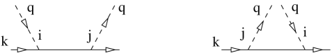
We now consider the calculation of those contributions that originate from the diagrams 9 and 10 of fig. 1, where a pion scatters inside a two-nucleon reducible loop. They are denoted by and , in order. As usual the diagram on the top corresponds to the direct part of the nucleon-nucleon scattering while that on the bottom represents the exchange part. The loop with the pions has to be corrected by initial (ISI) and final (FSI) state interactions, as denoted in the figure by the ellipsis which represent iterated nucleon-nucleon interactions. This iteration is the same as occurs for the nucleon-nucleon scattering in the nuclear medium, see fig. 6. The “elementary” nucleon-nucleon interaction is dressed by the iterative process which gives rise to eq. (4.5), with multiplied by the inverse of the matrix . In this way, if we denote by the elementary partial wave for a generic “production” process, , then the FSI dress it so that
| (6.1) |
The matrix , eq. (5.22), is already known from the study of the nucleon-nucleon interactions up to some order. On the other hand, can be fixed following an analogous procedure to that used before for determining in section 4.1. In this way, is determined by expanding eq. (6.1) in powers of up to and then comparing with a full CHPT calculation up to , with at most two-nucleon reducible diagrams. Note that we have written and because for our present purposes the basic process, made up by a two-nucleon reducible loop with the two pions attached to one nucleon propagator, starts at , so that , and it implies already one two-nucleon reducible loop. In addition, both ISI and FSI are involved in the diagrams 9 and 10 of fig. 1. Then, instead of eq. (6.1) we have
| (6.2) |
The LO result requires to employ and to calculate the two-nucleon reducible loop to which the two pions are attached by factorizing on-shell the nucleon-nucleon scattering amplitudes. We use the notation with the chiral order,
| (6.3) |
Explicit expressions for are given below in eqs. (6.11) and (6.14).

At NLO one has an extra two-nucleon reducible loop. Expanding the matrices in eq. (6.2) up to one and up to we obtain
| (6.4) |
We now match the previous equation with the result of fig. 15. In this figure we have included inside each loop the labels “exact” or “fact” according to whether the loop is calculated exactly or by factorizing on-shell the nucleon-nucleon vertices. The filled circle refers to the pion-nucleon scattering process that contains both the local and the Born terms, fig. 16. We denote by the two-nucleon reducible loop without external pions calculated exactly in CHPT and that occurs in figs. 15b and 15c. There is also the new contribution of fig. 15a whose exact calculation is denoted by . The result is
| (6.5) |
The equality of eqs. (6.4) and (6.5), taking into account eq. (6.3) for , implies that
| (6.6) |
In the last term we have the combination which is in our counting because it corresponds to the difference between an exact calculation of a two-nucleon reducible loop and that obtained by factorizing the vertices on-shell. The other contribution to is given by , as follows from eq. (6.6), that is also by the same token. Finally, note that in the previous expression the two pions are attached to the loops and , while the remaining terms originate because of nucleon-nucleon scattering.
The nucleon propagator before and after the filled circles in fig. 15 is the same so that it appears squared. This is required as the initial and final pion is also the same. We rewrite the nucleon propagator squared as
| (6.7) |
The filled circles in fig. 15 consists of a WT pion-nucleon vertex and of the pion-nucleon scattering Born terms shown in fig. 16. Its sum is
| (6.8) |
We do not include the in-medium part of the nucleon propagator in the previous equation because for the argument of the Dirac delta-function in eq. (3.2) is never satisfied as (nucleon kinetic energy). For the same reason, when performing the -integration in the loop, the poles at , resulting from eq. (6.8), are not considered because the nucleon propagators will not be any longer of but just of (standard counting). A contribution two orders higher would then result. Once the -integration is done the latter acquires from eq. (6.7) the value . The integration on for the evaluation of the two-nucleon reducible loop is analogous to the one performed in Appendix C for calculating the function. The point is that only depends on the energy of the external legs through the variable , eq. (5.7), that in turn only depends on the total energy. As a result, when the derivative with respect to acts on a baryon propagator not entering in eq. (6.8), one has
| (6.9) |
Taking into account the chiral expansion of the nucleon propagators involved in eq. (6.8) for the pole terms and summing with the WT term, we have the leading contribution
| (6.10) |
The antisymmetric tensor in eq. (6.10) gives rise to the isospin factor in the evaluation of the loops in fig. 15. Notice that in the loop the pions are attached to the propagators of the two nucleons, the upper and the lower ones, and these two contributions sum symmetrically. We can then rewrite eq. (6.3) for this case as
| (6.11) |
In these equations we have included the subscript given their isovector character. In the same way for one has
| (6.12) |
which corresponds to eq. (6.11) but substituting the term between brackets, where the nucleon-nucleon vertices are on-shell, by its exact calculation. By applying eq. (6.6) we can fix in terms of eqs. (6.11) and (6.12).
We now consider the case where the derivative with respect to from eq. (6.7) acts on the baryon propagators involved in the Born terms of eq. (6.8) with . The term can be neglected when summed with for our calculation to NLO, so that the derivative with respect to of eq. (6.8) yields the isoscalar contribution
| (6.13) |
For any the isospin identity operator gives rise to , instead of the factor of the isovector case. In this way, we can employ eqs. (6.11) and (6.12) substituting the vertex eq. (6.10) by eq. (6.13) and removing the action of the derivative . Thus,
| (6.14) |
Here the subscript is introduced given their isoscalar character. They give rise to . Notice that both and are one order higher than the analogous isovector terms in eqs. (6.11) and (6.12), respectively. This makes that starts to contribute at N2LO.
Next, we proceed to obtain the expressions for the pion self-energy corresponding to the diagrams 9 and 10 of fig. 1 as a sum over partial waves. The leading contribution is obtained by using , eq. (6.11), with the result
| (6.15) |
where the part corresponding to is the one proportional to in the previous equation. A symmetry factor 1/2 is included given the symmetry under the exchange of the two nucleonic external lines when they are finally closed.
In ref. [1] we established that at all the contributions to the pion self-energy involving nucleon-nucleon interactions vanish (). This implies that the contributions , , and must cancel mutually at this order. Recall that the isoscalar ones, and , are . The argument given in ref. [1] was a general one, without assuming any specific procedure for resumming the nucleon-nucleon interactions. We now show that UCHPT fulfills this requirement. When substituting into eqs. (5.16) and (5.18) the derivative eq. (5.24) at the lowest order, the following result is obtained
| (6.16) |
This equation is the same as eq. (6.15) but with opposite sign so that the cancellation with takes place.
In the following of this section we work out several N2LO contributions that comprise the isoscalar term as well those that are obtained by employing to NLO and in and , respectively. For the leading isoscalar contribution from , which is already due to the same reason as for , we obtain
| (6.17) |
Including one more order in the calculation of , and requires the use of , eq. (6.6). The input functions are given in eqs. (6.12) and (6.14) for the isovector and isoscalar cases, respectively. In this way,
| (6.18) |
It is straightforward to show that calculated with evaluated at NLO with eq. (5.24), , cancels with , eq. (6.18). One has to replace by its explicit expression in terms of , .
Let us mention that there is an extra term for
at . It
stems from a one more term to eq. (6.10) in the chiral
expansion
of the baryon propagators eq. (6.8). This contribution is
suppressed by the inverse of the large nucleon mass and will be considered when
a full N2LO calculation of the pion self-energy in the nuclear medium is
given. In Appendix B we evaluate explicitly and
needed for determining and ,
eqs. (4.13) and (6.6), in order. Some
steps introduced in the derivations of this and the previous section are also
calculated explicitly.
In summary, we have considered the calculation of the diagrams 9 and 10
of fig. 1, and , in order. We have shown explicitly that up to and
including NLO these contributions vanish with those evaluated in the previous section, and . Indeed, the cancellation obtained between these contributions in ref. [1] is more general because it was shown that once the Born terms in and are reduced to their leading contribution and summed to WT, as in eq. (6.10), the cancellation occurs. Some other contributions at N2LO have been also calculated, though they do not exhaust a full calculation to this order of the in-medium pion self-energy. It is then shown that at N2LO the just mentioned cancellation between the isovector contributions takes place as required by the findings of ref. [1]. Note that at this order the full calculation of the two-nucleon reducible loops takes place. This clearly shows that the cancellation is beyond the factorization approximation valid at NLO, as should be according to ref. [1].
7 Nuclear matter energy density

We study now the problem of the nuclear matter equation of state by applying eq. (2.5) up-to-and-including NLO. The diagrams required are shown in fig. 17. The first diagram corresponds to the energy of a free Fermi-sea. Its contribution, , is given by
| (7.1) |
and is the only contribution. Nonetheless, since this is a recoil correction originating from the first term of , eq. (3.5), one expects it to be suppressed numerically (it involves the inverse power of the hard scale instead of , the one in .) In addition, as shown below, there is further a dimensional suppression. Hence, the NLO contributions involving the nucleon-nucleon interactions, suppressed by just one extra chiral order, could be of comparable size. This is of course an important remark for the possible saturation of nuclear matter.
The NLO or contributions comprise the second and third diagrams. The former is the energy due to the one-pion loop nucleon self-energy whose expression, including a symmetry factor 1/2, is
| (7.2) |
The cut in from the free one-pion loop nucleon self-energy is restricted to the lower half-plane of the -complex plane, see eq. (3.16). In this way, by closing the first integral on the r.h.s. of the previous equation along an infinite semicircle centered at the origin and on the upper -complex plane, the contribution from the free part of cancels. Concerning the last term, an analogous reasoning to that given previously in connection with fig. 3 can be also applied here for the in-medium contribution of . This part is accounted for by the diagram 3.2 of fig. 17. Thus, the contribution that we keep now for the nuclear matter energy density from the second diagram of fig. 17, , is
| (7.3) |
Let us show that up to these two integrals give the same result. Taking into account the expression for the in-medium part of the one-pion loop nucleon self-energy, eq. (3.19), the first term on the r.h.s. of eq. (7.3) yields the integrals
| (7.4) |
where the order of the integrations have been changed. We perform the shift in the last integral, that is finite. In this way, eq. (7.4) can be rewritten as
| (7.5) |
If the higher order corrections from the difference are neglected in the previous equation, the last integral is the one defining , compare with eq. (3.16). Then, after summing over , we have the same contribution as the last one in eq. (7.3) up-to-and-including NLO. So finally we can write
| (7.6) |
Let us evaluate now the diagrams 3.1 and 3.2 of fig. 17, that collectively are denoted as diagrams 3 in the following. These diagrams fully involve the nucleon-nucleon scattering. Their contribution to the energy density, , is
| (7.7) |
In this expression we have explicitly shown the symmetry factor 1/2 and the sum over the spin () and isospin () labels, with .
The LO in-medium nucleon-nucleon scattering amplitude calculated in section 4.2 does not depend on . The interaction kernel only depends on at this order, while the resummation over the two-nucleon intermediate states, that gives rise to , Appendix C, depends on and as well. In the following we use as integration variables and introduced in eq. (5.6). The -integration from eq. (7.7) can be readily performed, with the result
| (7.8) |
Here, we have made use of the fact that only those terms with poles located in opposite halves of the -complex plane survive after the integration. Those terms with the two poles located at the same half of the -complex plane vanish, as it is clear by closing the integration contour with a semicircle at infinite along the other half. We insert eq. (7.8) into eq. (7.7), and use the variable , eq. (5.7), instead of . Thus,
| (7.9) |
where we made used that . The resulting redefinition of is not indicated as it is not relevant for the following manipulations, as well as the factor that is not shown. The first term between the square brackets on the r.h.s. of eq. (7.9) corresponds to the particle-particle part while the last one corresponds to the hole-hole part. Both of them originate by closing the nucleon lines in the diagrams 3 of fig. 17. Making use of
| (7.10) |
eq. (7.9) becomes
| (7.11) |
Let us discuss the calculation of the integral
| (7.12) |
This integral is involved in the first two terms of eq. (7.11). As a preliminary result let us discuss the particle-particle and hole-hole parts in , since they represent the inclusion of two-nucleon intermediate states in the medium. It is then convenient to express the function employing the first form of the nucleon propagator in eq. (3.2). In this way
| (7.13) |

Similarly as in eq. (7.8), only those contributions in eq. (7.13) with the two poles in lying on opposite halves of the -complex plane contribute. Then,
| (7.14) |
The first term is the particle-particle part and the last is the hole-hole one. Notice the different position of the cuts in . While for the particle-particle case has a negative imaginary part, , for the hole-hole part the cut takes values with positive imaginary part, . It is also worth mentioning that the extent of the cut in for the hole-hole part is finite. This cut in the last term of eq. (7.14) requires , but is bounded so that the two -functions in the numerator are simultaneously satisfied. The extension of this cut is given in eq. (C.19). We denote its lower limit by and its upper one by , corresponding to logarithmic branch points, where . This observation is very useful for performing the integral of eq. (7.12). For its evaluation we consider the contours and of fig. 18. The dashed line in the figure represents the cut in due to that in the hole-hole part of for and positive imaginary part . Physically it represents a real reshuffling of the occupied states by an in-medium pair of baryons respecting energy and three-momentum conservation. All the contours of integration include a semicircle at infinity centered at the origin along the upper part of the -complex plane. While the contour runs along the real axis, and then below the cut, the contour runs above it, with the imaginary part . In both cases the pole in the denominator of eq. (7.12) at is outside the contours of integration. Because of the convergent factor the integration along the semicircle at infinity is zero so that we can write
| (7.15) |
Since the cut is outside the contour , see fig. 18, the integration along this contour is zero
| (7.16) |
Subtracting eq. (7.16) to eq. (7.15) we are left with
| (7.17) |
Since the branch points are just of logarithmic type the integration along the vertical segments at and in fig. 18 do not contribute in the limit . Notice as well that the limit is already taken in the last line of eq. (7.17). The amplitude can be obtained from the analytical extrapolation in of the partial waves amplitudes
| (7.18) |
At LO depends only on , although for higher orders it could depend also on , and in addition to . We can also apply here eq. (5.15), keeping explicitly the separation between the and variables,
| (7.19) |
The analytical extrapolation in does not affect the expansion of the nucleon-nucleon scattering in spherical harmonics associated to the angular variables which are left intact. From eq. (7.18) it follows that
| (7.20) |
In this equation we have taken into account that although could depend on for higher orders, in the difference this dependence cancels. The point is that the discontinuity in due to the right-hand cut is fully taken into account by multiplying the loop function by the kernel on-shell, as in eqs. (4.5) and (4.31). The right-hand cut associated to the variable is then removed in the process of calculating order by order, as discussed in sections 4.1 and 4.2.
As commented above, the difference is due entirely to the hole-hole part of , the last term on the r.h.s. of eq. (7.14). From eq. (7.14) we have
| (7.21) |
Thanks to the -integration in eq. (7.17) is now trivial.#9#9#9The values of that satisfy the two in-medium -functions in eq. (7.21) for a given are comprised in the interval , which is the domain of the -integration in eq. (7.17). As a result eq. (7.11) turns into
| (7.22) |
where we have indicated explicitly the integration variables in the different functions. The isospin index and for one should take just one the two possible cases with , . It is straightforward to show that given in eq. (7.22) is purely real, as it should be. First, the two -functions in the first line of eq. (7.22) imply that only the hole-hole part of can have imaginary part. It follows that and since, furthermore, is a symmetric matrix (for the and partial waves) or just a number (for the rest of partial waves), the diagonal elements of the product
| (7.23) |
are positive real numbers. In this way we have for the imaginary part of ,
| (7.24) |
Taking into account eq. (4.31) and the expression for , eq. (7.14), the imaginary part of can also be calculated in terms of that of the hole-hole part of . Substituting the result in eq. (7.24), it follows that
| (7.25) |
The quantity between curly brackets in the previous equation is
| (7.26) |
But given and satisfying simultaneously the -functions in the first line, corresponding to two Fermi-sea insertions, it is not possible that they also satisfy simultaneously the two -functions in eq. (7.26), corresponding to the particle-particle part. Note that due to the Dirac -function in eq. (7.25) . As as result, it is clear that once eq. (7.26) is inserted in eq. (7.25).

Writing explicitly
| (7.27) |
we have for eq. (7.22)
| (7.28) |
The process followed from eq. (7.11) up to here can be schematically drawn as in fig. 19. The particle-particle part that results by closing the external lines in the diagrams 3 of fig. 17 is transferred to a reducible two-nucleon loop entering the in-medium nucleon-nucleon partial waves. This corresponds to the integration in in eq. (7.28), which is sandwiched between two partial waves amplitudes, one of them complex conjugated. The integration on in eq. (7.28) is linearly divergent because of the first integral on the second line. The product
| (7.29) |
tends to a constant for . Let us discuss how to regularize this integral, in the same way as already done for the calculation of the functions.
| (7.30) |
Let us denote by the limit for of . At LO this limit is a constant for each partial wave. Then, we rewrite the previous integral as
| (7.31) |
Now, since the integral
| (7.32) |
is convergent. The remaining integral in eq. (7.31) is expressed in terms of the function , eq. (4.7),
| (7.33) |
with
| (7.34) |
To simplify the notation let us define the symbols
| (7.35) |
The function depends on the same subtraction constant already employed in the study of the vacuum nucleon-nucleon interactions. The final expression for in eq. (7.28) is then
| (7.36) |
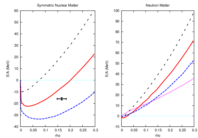
The sum of eqs. (7.1), (7.6) and (7.36) gives our result for the energy density, , in nuclear matter at NLO,
| (7.37) |
We evaluate eq. (7.36) using the in-medium nucleon-nucleon partial waves determined at LO in section 4.2. The sum over partial waves shows good convergence already for maximum and we sum up to . The results for the energy per nucleon, , are shown in fig. 20 for symmetric nuclear matter, left panel, and for neutron matter, right panel. The inserted point with errors on the left panel of fig. 20 corresponds to the experimental values for the saturation of nuclear matter MeV and fm-3 quoted in ref. [53]. The dotted line in the right panel is the result for neutron matter from the many-body calculation of the Urbana group [54]. It employs realistic nucleon-nucleon potentials and a fitted density dependent three-nucleon force in order to reproduce the experimental saturation point for nuclear matter. The rest of the curves, from top to bottom in both panels, correspond to the values of , and , in order.
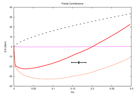
We observe that our curves for symmetric nuclear matter does have a minimum with a value in agreement with the experimental one, MeV, for . However, the position is displaced towards too low values of MeV, too small by a factor 1.7 compared with the value MeV [53]. For the case of neutron matter, the curves are repulsive and are larger than the calculation of the Urbana group [54] above some density. It is clear from fig. 11 and 12 that we are employing for the calculation of eq. (7.36) nucleon-nucleon partial waves that do not reproduce closely the Nijmegen data in several partial waves, see figs. 11-13. As commented above, we are just employing the iteration of the one-pion exchange and two four-nucleon local vertices. One needs more elaborate nucleon-nucleon partial waves. Indeed, there are many mutual cancellations involved in the case of symmetric nuclear matter, between the purely kinetic energy term, , and between the S- and P-waves in , with negligible small. Nevertheless, we find rather encouraging that our curves in fig. 20 can reproduce the main trends of both for symmetric nuclear and neutron matter despite they are obtained employing in-medium nucleon-nucleon amplitudes calculated only at LO. We already pointed out in section 4.1 that the one-pion exchange has a too large tensor force which is reduced by higher order counterterms (in the meson exchange approach this reduction is achieved by the exchange of -mesons [83].) In ref. [21] this point is emphasized in its study of nuclear binding because a large tensor force leads to less binding energy. Indeed, the partial waves - and have large matrix elements of the one-pion exchange tensor operator [21] and these partial waves are not well reproduced in our study at LO. We show in fig. 21 the different contributions to for symmetric nuclear matter and , that corresponds to the solid lines in fig. 20. Namely, , and are given by the dashed, dotted and dot-dashed lines, with the sum corresponding to the full curve. As expected, the contribution from , eq. (7.6), is very small since the derivative of with respect to is , as discussed in section 3.#10#10#10Notice that for and is very small. The other terms, and have similar size, though the former is and the latter . This is due to the fact that the kinetic energy term is a recoil correction stemming from , eq. (3.5), being suppressed numerically by the inverse of the large nucleon mass . Notice that scales like , which introduces, compared with , the additional power of times from the density and from . Both contributions have the same order of magnitude as the resulting factor . Additionally, there is also an extra suppression of the kinetic term contribution because of the dimensionality of space. The point is that contains the integral of , while the extra factor of density in goes like , so that a numerical factor is suppressing . Then, the cancellation between the kinetic energy term and the one due to the nucleon-nucleon interactions is a consequence of keeping the natural size for the chiral counterterms, of similar size than the one-pion exchange as seen in section 4.1. Of course, the precise value resulting from such cancellations depends on as shown in fig. 20. Additionally, the presence of such cancellation enhanced this dependence. E.g. for the neutron matter case the kinetic energy dominates the energy per baryon and the dependence on is smaller indeed. depends implicitly on through the nucleon-nucleon partial waves. Additionally, there is an explicit dependence from the first term on the last line of eq. (7.36), . The implicit dependence is due to the truncated solution of eq. (4.16), as discussed in detail in section 4.1. The explicit one should be also related to this truncation given the close similarity between them. To make this clear let us notice that the partial wave appearing in eq. (7.36) can also be written from eq. (4.31) as:
| (7.38) |
From the previous equation the term proportional to is
| (7.39) |
Then, a similar dependence on as that of results from eq. (7.39) as . The sum of both is . Thus, as a higher order calculation should dismiss the dependence on , by analogy, we expect this to be the case also for .
Another way of considering our power counting in eq. (2.5) is to use it for correcting order by order nucleon-nucleon amplitudes determined in vacuum. In this way, one can use better nucleon-nucleon partial waves, e.g. calculated at higher orders in momentum, and use in-medium corrections (whose calculation is always more cumbersome than diagrams in the vacuum) at lower orders. Another interesting issue left for further work is to explore the three-nucleon force influence on . This requires to consider the calculation of the energy density in the nucleon medium one order higher or , since .
7.1 Some phenomenology
In this section, we will give up the strict power counting scheme employed so far and try to analyse the possible effects of higher orders by some phenomenologically guided parameter fine-tuning. This will allow us to better understand the results obtained for nuclear and neutron matter in comparison to other recent studies, as e.g. in refs. [35, 31, 33].
As a first exercise, let us vary the parameter in order to improve the description of for the case of neutron matter, so that our results agree better with the dotted line in fig. 20 corresponding to the sophisticated many-body calculation of ref. [54]. The dashed line in fig. 22 is obtained employing . The so obtained fine-tuned curve is very close to the results of ref. [54], even up to rather high densities (the deviation is then less than 10.) Note as well that this result is obtained with a value of still of natural size, in the expected range around . However, if we employ the same for evaluating for symmetric nuclear matter the resulting curve has the minimum at its right position, fm-3, but the value of the energy per baryon is around MeV, which is an over-binding by a factor 2.5.
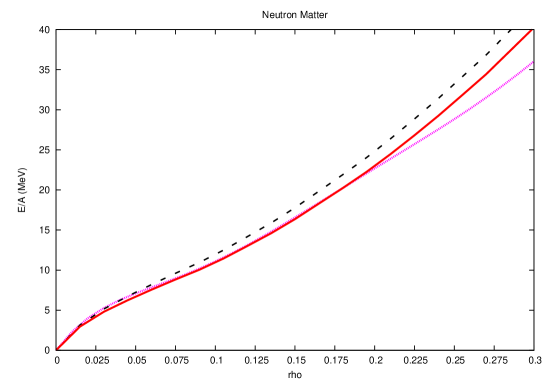
To further analyse the density dependence of nuclear matter, we rewrite the contribution from the interactions introducing by hand a new parameter, so that
| (7.40) |
Here we have distinguished between , that corresponds to the parameter that appears explicitly in because of the diverging integral in eq. (7.30), and , on which depends implicitly through the dependence on the nucleon-nucleon partial waves. The idea is to mock up higher order effects by varying independently and and exploit the phenomenological implications of such a procedure. While affects nucleon-nucleon scattering in vacuum, as discussed at length in section 4.1, affects only the nuclear matter equation of state. E.g. employing , which implies a change of with respect to used above, and that we also keep here, the solid curve in fig. 22 is obtained. The agreement for fm-3 between our results and ref. [54] is almost perfect.

For the case of symmetric nuclear matter the best results are obtained with , and . Again the magnitude of both numbers is of natural size. This is shown in fig. 23 by the two solid lines which have and , in order from top to bottom in the figure. The corresponding value for at the saturation point is and MeV, respectively. The experimental value given by the cross corresponds to MeV. The position of the minima for the same lines is and fm-3, compared to the empirical value fm-3. In addition, the dotted line is the result from the many-body calculation of ref. [54] employing realistic nucleon-nucleon interactions, that includes a free parameter to fix the three-nucleon interaction in the nuclear medium to reproduce the saturation point. We observe that our results reproduce very well the saturation point and agree closely with the calculation of ref. [54].
As done in ref. [31] it is illustrative to compare our curves in fig. 23 with the following simple parameterization for the energy per baryon in symmetric nuclear matter
| (7.41) |
Interestingly, the nuclear matter incompressibility [85, 86]
| (7.42) |
is correctly given once and are known by adjusting the empirical nuclear matter saturation point. In this equation is the Fermi momentum at the saturation point. For the central values of the point in fig. 23, fm-3 and MeV, the resulting nuclear matter incompressibility is MeV, which is compatible with the experimental value MeV [85]. Our curves can be also described rather accurately by eq. (7.41), as shown by the dashed curve in fig. 23 obtained by adjusting the minimum position and value of the lowest of solid curves. Both curves run very close to each other and start to deviate for densities above fm-3. The resulting nuclear matter incompressibility calculated from our results is and MeV, for the upper and lower solid curves, respectively. These values are compatible with the experimental value. The close agreement between our results and eq. (7.42) shows that, to a good approximation, the former admits an expansion in powers of the Fermi momentum as in eq. (7.41) for low .
In Table 1 we show the contributions to (MeV) in nuclear matter for the different partial waves considered at the saturation point fm-3. The first column to the right of every partial wave corresponds to and the second one to , and is fixed to in the two cases. The former case is the top solid line in fig. 23 and the latter is nearly the dot-dashed line in the left panel of fig. 20. The kinetic energy contributes with MeV per nucleon. One observes clearly the dominant role of the S-, P- and waves. It is remarkable the large influence of the medium on the partial wave that despite being attractive in vacuum gives a repulsive contribution in the medium for , and only slightly attractive for . The change of the contribution with is due to the fact that for the phase shifts decrease with energy (they are 30 and 20 degrees at and MeV, respectively), instead of stabilizing at around 60 degrees like happens for , see fig. 11. In this way, its contribution is less attractive. We also remark that the non-elastic partial waves, e.g. the , also contribute to from and and are included in the elastic ones. For a given partial wave they correspond to one term in the sum of two terms on in eq. (7.35).
Thus, we are able to reproduce the equation of state of symmetric and neutron matter in terms of one fine-tuned free parameter, the value of for the symmetric nuclear matter case. The parameter comes out always with a value close to the expected one, . For neutron matter one has and for symmetric nuclear matter . In addition, it is worth stressing that the resulting values for are all negative with the appropriate size, so it is justified to solve approximately eq. (4.16) making use of UCHPT. We think that this achievement is not a trivial fact and clearly indicates that our power counting, eq. (2.5), is able to map out properly the important dynamics in the nuclear medium and establish a useful hierarchy to allow for systematic calculations. At present, the strong dependence on of particularly the and partial wave contributions, see Table 1, seems to indicate that in order to go forward in the application of our chiral power counting eq. (2.5), one should consider the exact solution of , eq. (4.16), and not its truncated solution in powers of , eq. (4.10), as presently done. Notice that in comparison with refs. [35, 31, 33], that also applies Baryon CHPT to in-medium calculations, we employ the same approach both for vacuum and nuclear matter calculations and are able to compare with nucleon-nucleon scattering data.
8 Conclusions
In [1] we derived a novel approach for an EFT in the nuclear medium based on a chiral power counting that combines both short-range and pion-mediated internucleon interactions. The power counting is bounded from below and at a given order it requires the calculation of a finite number of contributions, which typically implies the resummation of an infinite string of two-nucleon reducible diagrams with the leading multi-nucleon CHPT amplitudes. These resummations arise because this power counting takes into account from the onset the presence of enhanced nucleon propagators and it can also be applied to multi-nucleon forces. However, ref. [1] did not discuss any specific non-perturbative method for applying this novel counting scheme to practical calculations. We have developed in the present paper the required non-perturbative technique that allows us to perform these resummations both in scattering as well as in production processes. This non-perturbative method is based on Unitary CHPT, which is adapted now to the nuclear medium by implementing the power counting of ref. [1]. We have first applied it to calculate the LO and NLO vacuum nucleon-nucleon interactions. There, we have also shown the tight connection between the UCHPT approach and dispersion relations for the nucleon-nucleon scattering amplitude. The former results as an approximate solution to the dispersive treatment of nucleon-nucleon scattering in a chiral expansion of the imaginary part of the scattering amplitudes along the left-hand cut, taking advantage of the suppression of the two-nucleon unitarity loops along this cut. It was also shown that the subtraction constant , employed for regularizing the reducible part of the two-nucleon reducible loops, realizes a convenient splitting between loops and tree-level contributions, while the exact solution for nucleon-nucleon scattering in vacuum has been shown not to depend on . For the in-medium case the LO nucleon-nucleon scattering is given as well. Then, the pion self-energy in nuclear matter up to was determined together with some other contributions at N2LO. The cancellation found in ref. [1] between all leading corrections to the linear density approximation for the pion self-energy is explicitly shown here for the amplitudes calculated utilizing the non-perturbative method developed here up to N2LO, which is a good check for the consistency of our approach. We have also addressed the calculation of the energy density of nuclear matter . The non-perturbative technique developed gives rise to different contributions to whose imaginary parts cancel between each other and a real value results, as it should. We obtain saturation in symmetric nuclear matter and repulsion for neutron matter. The contributions from the nucleon-nucleon interactions are of similar size to those from the kinetic energy term, the latter being suppressed by the inverse of the large nucleon mass and a dimensional factor. It is remarkable that we obtain for a very good reproduction of sophisticated many-body calculations that employ realistic nucleon-nucleon potentials for the equation of state of neutron matter up to rather high nuclear densities. We can also achieve such a good agreement for the case of nuclear matter by allowing to distinguish between and , where the former parameter appears explicitly in the calculation of the energy per baryon while the latter appears implicitly through the nucleon-nucleon scattering amplitudes involved. By this splitting, we can mock up the effects of higher orders. The parameter can be fixed from the neutron matter equation of state. We then obtain a very accurate reproduction to as function of density in symmetric nuclear matter for , with saturation at fm-3 and MeV, cf. the experimental values fm-3 and MeV. Furthermore, the nuclear matter incompressibility comes out with a value between 240-250 MeV, in perfect agreement with the experimental one of MeV. We interpret the success of our reproduction of the nuclear matter equation of state for both symmetric and neutron matter in terms of one free parameter for each of them as an indication that our power counting is a realistic one and that it is able to establish a useful hierarchy within the many contributions and complications inherent to nuclear dynamics. This opens the way to proceed systematically improving the calculations in a controlled way.
Certainly, higher chiral orders should be worked out to obtain more precise results concerning the interesting problems considered here. In particular, it would be desirable to solve exactly eq. (4.15) in order to have free nucleon-nucleon partial wave amplitudes independent of . In addition, a N2LO calculation will address the interesting question about the importance of three-nucleon forces for nuclear matter saturation. Similarly, a N2LO calculation of the pion self-energy is a very interesting task. It will merge important meson-baryon mechanisms like e.g. the Ericson-Ericson-Pauli rescattering effect [45], with novel multi-nucleon contributions that can be worked out systematically within our EFT. More calculations and applications of the present theory to other interesting physical problems should be pursued.
Acknowledgements
We would like to thank Andreas Wirzba for discussions. This work is partially funded by the grant MEC FPA2007-6277, by BMBF grant 06BN9006, EU-Research Infrastructure Integrating Activity “Study of Strongly Interacting Matter” (HadronPhysics2, grant n. 227431) under the Seventh Framework Program of EU, HGF grant VH-VI-231 (Virtual Institute “Spin and strong QCD”) and by DFG (TR-16 “Subnuclear Structure of Matter”).
Appendix A Partial wave decomposition of in-medium nucleon-nucleon amplitudes
In this appendix, we derive the partial wave decomposition of the nucleon-nucleon scattering amplitudes in the CM frame. Our states are normalized as,
| (A.1) |
Here, corresponds to the total four-momentum of the final state and to that of the initial one, with , the total CM energy. In addition, and are the energies of the particles 1 and 2, in order. The indices and refer to any discrete quantum number required to characterize the states. In the CM frame the solid angle is denoted by and the modulus of the three-momentum by . The two-particle states with well-defined orbital angular momentum are defined as,
| (A.2) |
Taking into account eq. (A.1) it follows then
| (A.3) |
The decomposition into states with well-defined total angular momentum , third component , orbital angular momentum and total spin is given by,
| (A.4) |
where the indices and refer to the third components of spin, and to their maximum values and to the third component of the orbital angular momentum .#11#11#11Strictly speaking in order to match with the normalization in eq. (4.6) we should multiply the right-hand-side of eq. (A.4) by . This is a relativistic correction of . Next, we introduce the isospin indices , , for the third components, , , for their maximum values, and decompose the free state in terms of states with well-defined total isospin and third component . In addition, the antisymmetric nature of a two-fermion (two-nucleon) state is introduced,
| (A.5) |
with the repeated indices to be summed. This convention is used throughout this section. To simplify the notation we denote the left-hand-side of the previous equation as , with the subscript indicating that the state is antisymmetrized. Applying the relations [84] , , and analogously for isospin, eq. (A.5) for the nucleon-nucleon case () simplifies to
| (A.6) |
with
| (A.7) |
In this way, ensures the well known rule that must be odd for any partial wave. Using the decomposition eq. (A.6) we have for the scattering amplitude,
| (A.8) |
Here, is the partial wave with final total angular momentum , initial one , final total spin , initial one , isospin and final and initial orbital angular momenta and , respectively. Notice that in the previous equation we have distinguished between the final and initial total angular momenta and , and similarly for the total spins and . For free two nucleon scattering we have of course because of angular momentum conservation. This conservation law, the conservation of parity and the rule odd imply that . However, the resulting matrix elements in the nuclear medium depend additionally on the total three-momentum of the two nucleons because the medium rest-frame does not coincide in general with their center-of-mass. This is why we have included as an argument in the scattering operator, with the former defined in (5.6). Employing the orthogonality properties of the Clebsch-Gordan coefficients and spherical harmonics, one can invert eq. (A.8) with the result,
This expression can be further reduced by making use of properties under rotational invariance so that the initial relative three-momentum can be taken parallel to the -axis. In deriving this simplification we omit the isospin indices that do not play any role in the following considerations, and introduce the symbol
| (A.10) |
Now consider the rotation , such that , that consists first of a rotation around the -axis with an angle and then a rotation around the -axis with an angle , where and are the polar and azimuthal angles of , respectively. We could also have taken first an arbitrary rotation of angle around the -axis. Then,
| (A.11) |
with and . The dependence on the total three-momentum has been made explicit in the state vectors to emphasize that the total three-momentum also is rotated. Inserting eq. (A.11) into eq. (LABEL:pw.d2.i1) we have,
| (A.12) |
The spherical harmonics satisfy the following transformation properties under rotations,
| (A.13) |
Inserting these equalities into eq. (A.12) we are then left with the following product of rotation matrices,
| (A.14) |
We now take into account the Clebsch-Gordan composition of the rotation matrices [84],
| (A.15) |
Since eq. (A.14) appears in eq. (A.12) times Clebsch-Gordan coefficients we can make use of the previous composition repeatedly. First,
| (A.16) |
The rotation matrix , that appears on the right-hand-side of the first of the previous equalities, can then be combined in eq. (A.12) such that
| (A.17) |
Similarly
| (A.18) |
Incorporating eqs. (A.17) and (A.18) in eq. (A.12), the latter takes the form
| (A.19) |
Let us first consider the vacuum case where the scattering amplitude does not depend on . In this way the integration over in the previous equation can be done explicitly taking into account the orthogonality relation between two rotation matrices [84]. For that let us recall our previous remark about the fact that an arbitrary initial rotation over the -axis and angle can also be included. In this way we take
| (A.20) |
Inserting this back to eq. (A.19) one arrives at
| (A.21) |
In this expression we have made use that only gives a contribution to and, as explained after eq. (A.8), . In addition, we have also used that , since both vectors are related by a rotation. The subscript in is suppressed because and it is redundant. Also, we have employed the notation for the partial waves of section 4, .
We now come back to the in-medium case and keep the dependence on . Here also so that . Let us show first that a Fermi-sea with all the free three-momentum states filled up to has total spin zero. This is required because for a given three-momentum one has two spin states that must be combined antisymmetrically because of the Fermi statistics so that for this pair. Then, since this happens for any pair, the total spin of the Fermi sea must be zero. Regarding total angular momentum we now give a non-relativistic argument to claim that the orbital angular momentum must also be zero. This is due to the fact that the nuclear medium in the CM of the two nucleons that scatter is seen with a velocity parallel to . In this way, both the CM position vector and the total three-momentum of the nuclear medium are also parallel so that their cross product vanishes. As a result, since the intrinsic orbital angular momentum of the medium is also zero, one expects that the total angular momentum is zero for the system also in the CM frame of the two nucleons. Thus, also in this case and then, because of the same reasons as in vacuum, . Let us recall the remark after eq. (5.15) to justify that is conserved also in the nuclear medium. In addition the third component of total angular momentum must be conserved, , and summing over one has
| (A.22) |
given the unitary character of the rotation matrices. Then,
| (A.23) |
This expression reduces to the one in the vacuum, eq. (A.28), whenever the integral
| (A.24) |
does not dependent on . In that case the integration over is simply and eq. (A.21) is restored.
Eq. (A.23) can be further simplified because for the evaluation of a nucleon-nucleon partial wave amplitude one only needs to consider the direct term in the nucleon-nucleon scattering amplitude. This follows because the operator is Bose-symmetric so that,
| (A.25) |
When implementing the second or exchange term in eq. (A.23), re-including the isospin indices as well, and using the above referred symmetry properties of the Clebsch-Gordan coefficients and spherical harmonics, one is left with the same expression as for the direct term in eq. (A.25) except for the global sign . Summing both expressions the factor
| (A.26) |
arises. Given the definition of in eq. (A.7) and imposing the rule that odd and odd, the factor can be simplified on both sides of eq. (A.23). The latter then reads
| (A.27) |
with only the direct term, as indicated by the subscript in the scattering operator. For the particular case of the vacuum nucleon-nucleon scattering the previous expression simplifies to
| (A.28) |
Appendix B Explicit calculation of and up to
In this section we evaluate explicitly and since they enter for fixing and , eqs. (4.13) and (6.6), respectively. We also show with explicit calculations some of the steps introduced in the derivations of sections 5 and 6. For the calculation of these diagrams one has to recall that the exchange of a wiggly line corresponds to local plus one-pion exchange terms, fig. 5. When the nucleon loop, to which the two pion lines are attached, includes only nucleon-nucleon local vertices, we then have and for the isovector and isoscalar cases, respectively. At the same order, when one of the nucleon-nucleon vertices in this loop corresponds to a one-pion exchange then and result. Finally, when both vertices are due to one-pion exchange one has and .

We first consider the two-nucleon reducible loop with only local vertices, fig. 24. For the isovector case the derivative with respect to from eq. (6.7) acts on a nucleon propagator not entering in eq. (6.8). With the four–nucleon local vertex of eq. (4.2) we then have for ,
| (B.1) |
where . The spin indices are indicated with Greek letters. The momentum integration is the same as for the function , eq. (C.1), so that a factor results. The previous equation contains both the direct and exchange terms, though the direct term is the one needed to evaluate the different partial waves. Notice that the previous equation only contributes to the S-waves. We now work out the spin projections of the direct term in eq. (B.1) with the result
| (B.6) |
As it should, we have then the combinations and for and 1, respectively. The isospin projection corresponding to the operator is , which excludes altogether. Keeping only the direct term in eq. (B.1) , we have
| (B.7) |
For the isoscalar contribution we just have to remove the derivative and replace the vertex of eq. (6.10) by eq. (6.13). The spin projection is the same as before, eq. (B.6). However, the isospin operator now is different and for the direct term just corresponds to twice the identity operator. As a result
| (B.8) |
and both and 1 contribute. In and there is no dependence on , they depend only on , so that one can calculate the projection into the S-waves as in vacuum, making use of eq. (A.28).
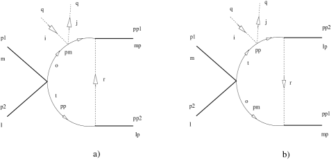

We now consider and , with one local and one-pion exchange vertices. The isovector contribution corresponds to fig. 25, , and fig. 26, , depending on whether the one-pion exchange is between the final or initial two nucleons, respectively. For the sum of the diagrams in fig. 25 one has
| (B.9) |
where the repeated indices are summed and .
Instead of keeping we take
, with , as done
in eq. (6.7). On the other hand, for the pion propagator we neglect
its dependence on , since it is
, while is . Then, the energy dependence
enters in similarly as in and the derivative can be taken
with
respect to the variable , eq. (6.9), with after the
derivative is performed. Let us consider the isospin and spin projections for
the direct term, given by the first square bracket in the previous equation.
The isospin operator
has a
projection between states of well defined isospin given by .
The spin operator, after some algebraic manipulation in the term
proportional to , reads
| (B.10) |
The structures and are already projected in eq. (B.6) for the different spin states. There is, however, the new structure whose matrix elements are
| (B.15) |
In this matrix the rows correspond to the final third component of the total spin, , and the columns to the initial one, . Then, we can write for the direct term with total spin
| (B.16) |
using eqs. (B.9) and (B.15). In the integrals of eqs. (B.16) it is convenient to perform the shift of the integration variable
| (B.17) |
which implies that
| (B.18) |
For the one-pion exchange between the initial nucleons, fig. 26, we proceed in the same way followed for above. Performing the same transformation in the integration variable as in eq. (B.17), the expressions for can be used for with the exchange of .
We now introduce the functions , and defined as
| (B.19) |
with . These integrals are further discussed in Appendix D. In terms of the functions introduced in eq. (B.19) one can write the different matrix elements of as
| (B.20) |
| (B.21) |
The isoscalar contribution originates by taking the derivative of the intermediate nucleon propagator in fig. 16. We have the same expression as for , eq. (B.9), but removing the operator and with the replacement
| (B.22) |
As a result, the isospin operator changes and for the direct term it is given now by
| (B.23) |
The projection for a state with is . For there is now a contribution from eq. (B.23) given by
| (B.24) |
Hence, instead of eq. (B.16), we arrive at
| (B.25) |
such that for and , for . Similar expressions to eq. (B.21) can be written. E.g. for one has now
| (B.26) |
Here, the tilde indicates the symmetric form
| (B.27) |
with and given in terms of as explained above. The expressions for are the same as those worked out for with the replacement , as noted above for the amplitudes.
Let us consider the partial wave projection of and . As discussed at the end of Appendix A, we can still use eq. (A.28), valid in the vacuum, if the integral in eq. (A.24) does not depend on . For and , with the one-pion exchange between the final nucleons, this is clearly the case because and only depend on through its scalar product with . Thus, there is no angular dependence left on once the integration over is performed. For the case when the pion is exchanged between the initial nucleons, fig. 26, the resulting and do not depend on the final three-momentum . In this way, the integration over cannot remove the dependence on . This also implies that this diagram only can contribute to partial waves with , that is, and . However, as remarked above after eq. (B.18), the exchange transforms , into , and vice versa. In addition, one has to notice the symmetry between and in eq. (LABEL:pw.d2.i1) for the partial wave decomposition. It is then clear that the same partial waves result for the diagrams of figs. 25 and 26 with the exchange . Thus, we can still use eq. (A.28) but using the diagrams with the pion exchanged between the final nucleons. The elastic partial wave is exactly the same for both diagrams and is equal to evaluated as discussed. We denote the corresponding partial waves by and . For , that requires , only the partial wave is not zero. On the other hand, for both isospin combinations occur. Then one has the partial waves , , and . We have the following expressions for , omitting the subscripts 12 or 13,
| (B.28) |
Let us recall that in order to apply the previous equations, the vector must be taken along the axis. Namely, for the partial wave projections, we take the reference frame with the axes
| (B.29) |
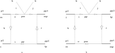
Let us move now to the evaluation of and where both vertices in the two-nucleon reducible loop at which the two pions are attached correspond to one-pion exchange. As in the previous cases we start by calculating the isovector case. We restrict ourselves from the beginning to the direct contribution, corresponding to the diagrams in fig. 27, whose sum is
| (B.30) |
The diagonal matrix elements of the isospin operator
| (B.31) |
present in eq. (B.30), are given between states with well defined isospin as
| (B.32) |
which is zero for . With respect to spin we can rewrite,
| (B.33) |
The matrix elements of the spin operators and between states with well defined total spin were already worked out in eqs. (B.6) and (B.15), respectively. We have now in addition the operator
| (B.34) |
whose matrix elements are
| (B.35) |
and 0 for . We follow in the previous matrix the same notation as in eq. (B.15). Taking into account this matrix and eqs. (B.6) and (B.15) one can determine the operator of eq. (B.33) between two-nucleon states with well defined third component of total spin . The latter are inserted into eq. (B.30) together with the isospin factor , eq. (B.32). As a result, the amplitudes and are determined.
The isoscalar contributions arise by taking the derivative of the intermediate nucleon propagator in fig. 16 with respect to , as discussed in eq. (6.13). We have the same expression as for , eq. (B.30), but removing the derivative and with the replacement of eq. (B.22). The resulting isospin operator is now given by
| (B.36) |
One can work out straightforwardly its diagonal matrix elements between states with definite isospin,
| (B.37) |
with . Then, instead of eq. (B.30) one has now,
| (B.38) |
with as before. The tensor integrals required by eqs. (B.30) and (B.38) that involve one intermediate two-nucleon state with two one-pion exchanges are calculated in Appendix E.
To determine the partial waves for and we have checked numerically that eq. (A.24) does not depend on at the level of one per mil. This is similar to the numerical accuracy to which the in-medium integrations have been calculated. As a result, we can use the same equation for partial wave projection as in vacuum, eq. (4.4), but now in terms of and . This reduces the calculational load because eq. (4.4) has not the integration over as in eq. (A.27). We denote by and the resulting partial waves for and , in this order.
Summing over the previous partial waves it follows that
| (B.39) |
Comparing with eq. (6.14) it is straightforward to determine .
Appendix C The loop function
The function is given by
| (C.1) |
This integration corresponds to the loop in fig. 7 with total in-coming four-momentum . In the following we define,
| (C.2) |
The different contributions to are calculated according to the number of in-medium insertions in the nucleon propagators, eq. (3.2). The -integration for the free part, , is performed by applying Cauchy’s theorem,
| (C.3) |
with given in eq. (5.7). One has to keep in mind in the following the prescription in the definition of . In order to emphasize this, we will write explicitly the combination in many integrals, though the is already contained in according to eq. (5.7). The result in eq. (C.3) corresponds to eq. (4.9) that is regularized according to the dispersion relation eq. (4.7),
| (C.4) |
For the one-medium insertion, the -integration is done by making use of the energy-conserving Dirac delta-function in the in-medium part of the nucleon propagator, eq. (3.2). We are then left with
| (C.5) |
Let us concentrate on the evaluation of the integral,
| (C.6) | ||||
Here, we have taken into account that the Heaviside function in the numerator implies the conditions,
| (C.7) |
Despite the separation between the cases and , both give rise to the same expression in eq. (C.6). In terms of the function , eq. (C.5) reads
| (C.8) |
For the case with two medium insertions
| (C.9) |
Here we assume that . If the opposite were true one can use the same expressions that we derive below but with the exchange . This is clear after changing in the integral of eq. (C.9). Denoting by the angle between and the two step functions require
| (C.10) |
One has to impose that and , otherwise is out of the range . In addition, it is also necessary that .
| (C.11) |
The simultaneous consideration of the first and third of the previous conditions requires that for , which in turn implies
| (C.12) |
Notice that the previous upper bound is larger than because . From eq. (C.12) it follows then that , and since it is always the case that the second condition in eq. (C.11) is satisfied. On the other hand,
| (C.13) |
For the final form of one also has to take into account the conditions,
| (C.14) |
Gathering together the conditions in eqs. (C.10)–(C.14) we have the following options,
| (C.15) |
which is not possible because . Also
| (C.16) |
This only holds for . Then and . Further
| (C.17) |
In this case, and . It follows that for and for . In both cases , as can be easily seen. The last possibility is
| (C.18) |
For this case to hold, it is necessary that . But then so that the allowed upper limit for is not . In this case, and . In summary,
| (C.19) |
As a technical detail one can take directly the derivative of eq. (C.19) with respect to for a given interval. The different intervals do not imply the appearance of delta functions of when differentiating as one check by evaluating directly the derivative of eq. (C.9).
Appendix D Calculation of , and
We now consider the integrals defined in eq. (B.19), though we calculate here completely only the scalar integral . For the calculation of and one resorts to the Passarino-Veltmann reduction and explicit calculations and expressions are given in ref. [63]. Nevertheless, we evaluate at the end of this Appendix the free part of the tensor integral in order to explicitly show how to handle the regularization of a two-nucleon reducible loop different to in terms of .
We evaluate according to the number of in-medium insertions. After performing the -integration by applying Cauchy’s theorem we are left for the free part with
| (D.1) |
In the previous equation, we have introduced a Feynman integration parameter as an intermediate step and for . For the one-medium insertion case, the -integration is straightforward due to the presence of the energy Dirac delta-function
| (D.2) |
Both terms in the sum can be obtained from the function
| (D.3) |
Let us work out the scalar product . For the integration, we introduce the reference frame
| (D.4) |
From the last relation we have,
| (D.5) |
with and integration variables in eq. (D.3) and . Let us perform the -integration,
| (D.6) |
that also has been checked numerically. In eq. (D.6) we have
| (D.7) |
where . Next, we move to the integration of eq. (D.3). For this integration one has to take into account the presence of the Heaviside function, which implies the conditions already worked out in eq. (C.7). The latter determine an interval of integration for for a given value of . Then, we can write,
| (D.8) |
with
| (D.9) |
Now, we consider the final integration on in eq. (D.2) and define the auxiliary function,
| (D.10) |
in terms of which eq. (D.3) reads
| (D.11) |
Then from eq. (D.2) one has
| (D.12) |
Here, we have only indicated those arguments that change for each term in the sum of eq. (D.2) to calculating . Indeed, depends also on and . The integration over when two medium insertions are represent can be done straightforwardly because of the additional Dirac delta-function of the energy that fixes . Then,
| (D.13) |
We have the same -integration as in eq. (D.6), with the same result but now with . The integration over is the same as in eq. (D.8), though with a different integration interval for that is fixed by the values of and , according to the results of section C. They are collected here for ,
| (D.18) |
with and defined in eq. (C.11). We also define, similarly as was done for , the auxiliary function
| (D.19) |
with for the values of , and in eq. (D.9) and and according to eq. (D.18). In this way,
| (D.20) |
For the case the change of variable is performed in eq. (D.13) and thus
| (D.21) |
Let us now consider the calculation of corresponding to
| (D.22) |
We now multiply the previous equality by and sum over repeated indices, then
| (D.23) |
Doing first the angular integration, one has
| (D.24) |
Let us consider the expansion of the last factor in the previous equation for ,
| (D.25) |
Adding and subtracting to eq. (D.24) it results
| (D.26) |
The first integral is convergent because of the expansion in eq. (D.25) while the second one corresponds to , eq. (4.7).#12#12#12From a practical point of view it is simpler to calculate algebraically the initial integral eq. (D.23) in cut-off regularization than the convergent one eq. (D.26). Then, the cut-off is sent to infinity while keeping only the divergent linear term. The cut-off can be expressed in terms of by proceeding in the same way for in eq. (4.7).
Next, we multiply eq. (D.22) by , sum over and and proceed in the same way as before. After performing the angular integration we have
| (D.27) |
As in eq. (D.25) we consider the limit of the last factor in the integrand for
| (D.28) |
Adding and subtracting the first term on the r.h.s. of the previous equation, similarly as done in eq. (D.26), we have a convergent and a divergent integral. The convergent one is given by
| (D.29) |
while the divergent integral corresponds to
| (D.30) |
The calculation of the integrals eqs. (D.23) and (D.27) explicitly shows how to regularize in terms of the subtraction constant the linear divergences present in the calculation of the two-nucleon reducible loop integrals needed for the evaluation of the loops in figs. 25, 26 and 27. Since two pion exchanges are involved in the latter figure only the scalar integral with in the numerator, denoted by , diverges. Its divergent part can be straightforwardly regularized in terms of , as in eqs. (D.26) and (D.30). Indeed, it just corresponds to .
Appendix E Calculation of
The different integrals involved in the evaluation of and can be expressed in terms of a set of scalar integrals. The tensor structure of these integrals is determined by the matrix elements in eq. (B.33). We also perform here the shift of the integration variable as in eq. (B.17), and rewrite eqs. (B.30) and (B.38) accordingly. The integrals necessary for the calculation of the latter equations are evaluated in ref. [63]. Here, we only discuss the calculation of the basic scalar integral involved, . For integrals with more complicated tensor structure one uses the Passarino-Veltmann reduction. In the expressions that follow it is always assumed that the -integration has been done either by using Cauchy’s theorem, for the free part, or employing the energy Dirac delta-functions from the in-medium insertions. On the other hand, since now two pion propagators are involved we join them in one introducing a Feynman parameter
| (E.1) |
with
| (E.2) |
where
| (E.3) |
In order to apply the results already derived in Appendix D, where only one pion propagator was involved, we take into account that
| (E.4) |
as it follows from the definition of in eq. (E.2). The scalar function is defined by
| (E.5) |
For the free part
| (E.6) |
The integration over was already done in eq. (D.1). Making use of this result one has
| (E.7) |
with . For the part with one-medium insertion
| (E.8) |
The two terms in the sum can be obtained from the function
| (E.9) |
This integral is analogous to in eq. (D.3), but with and replaced by and , in that order. Furthermore one of the factors in the denominator is squared. Following the calculation of , we adopt the reference system
| (E.10) |
with
| (E.11) |
so that the scalar product , where and are the polar and azimuthal angles of . Let us perform the -integration in eq. (E.9)
| (E.12) |
The last integral is of the type already evaluated in eq. (D.6) where now
| (E.13) |
with as in eq. (D.9). Then, eq. (E.12) reads
| (E.14) |
The integration of the previous result includes the Heaviside function in eq. (E.9) that fixes the limits of integration to and given by eq. (C.7). This integration is straightforward, see e.g. the similar one of eq. (D.8). Then, our result for is
| (E.15) |
Here we have used the function
| (E.16) |
For the function of eq. (E.8) we have , with .
| (E.17) |
The angular integrations are of the same type as already developed for the case of the one-medium insertion and, hence, we define
| (E.18) |
with the integration limits given in eq. (D.18), where it is assumed that . In terms of this function . When we perform, as usual, the change of variables in eq. (E.17) and then .
References
- [1] J. A. Oller, A. Lacour and U.-G. Meißner, J. Phys. G 37 (2010) 015106.
- [2] S. Weinberg, Physica A 96 (1979) 327.
- [3] S. Weinberg, Phys. Lett. B 251 (1990) 288.
- [4] S. Weinberg, Nucl. Phys. B 363 (1991) 3.
- [5] C. Ordonez, L. Ray and U. van Kolck, Phys. Rev. C 53 (1996) 2086.
- [6] U. van Kolck, Prog. Part. Nucl. Phys. 43 (1999) 337.
- [7] D. R. Entem and R. Machleidt, Phys. Rev. C 68 (2003) 041001.
- [8] E. Epelbaum, W. Gloeckle and U.-G. Meißner, Nucl. Phys. A 671 (2000) 295; Nucl. Phys. A 747 (2005) 362.
- [9] E. Epelbaum, H. Kamada, A. Nogga, H. Witala, W. Gloeckle and U.-G. Meißner, Phys. Rev. Lett. 86 (2001) 4787.
- [10] E. Epelbaum, Prog. Part. Nucl. Phys. 57 (2006) 654.
- [11] E. Epelbaum, H. W. Hammer and U.-G. Meißner, Rev. Mod. Phys. 81 (2009) 1773.
- [12] D. B. Kaplan, M. J. Savage and M. B. Wise, Nucl. Phys. B 534 (1998) 329; Phys. Lett. B 424 (1998) 390.
- [13] S. Fleming, T. Mehen and I. Stewart, Nucl. Phys. A677, (2000) 313; Phys. Rev. C 61 (2000) 044005.
- [14] S. R. Beane, P. F. Bedaque, M. J. Savage and U. van Kolck, Nucl. Phys. A 700 (2002) 377.
- [15] A. Nogga, R. G. E. Timmermans and U. van Kolck, Phys. Rev. C 72 (2005) 054006.
- [16] E. Epelbaum and U.-G. Meißner, arXiv:nucl-th/0609037.
- [17] M. Pavon Valderrama and E. Ruiz Arriola, Phys. Rev. C 70 (2004) 044006.
- [18] E. Epelbaum and J. Gegelia, Eur. Phys. J. A 41 (2009) 341.
- [19] J. Soto and J. Tarrus, Phys. Rev. C 78 (2008) 024003.
- [20] P. Saviankou, S. Krewald, E. Epelbaum and U.-G. Meißner, arXiv:0802.3782 [nucl-th].
- [21] R. Machleidt, P. Liu, D. R.Entem and E. Ruiz Arriola, arXiv:0910.3942 [nucl-th].
- [22] R. J. Furnstahl, G. Rupak and T. Schäfer, Ann. Rev. Nucl. Part. Sci. 58 (2008) 1, and references therein.
- [23] S. K. Bogner, R. J. Furnstahl, A. Nogga and A. Schwenk, arXiv:0903.33661 [nucl-th].
- [24] S. K. Bogner, R. J. Furnstahl, S. Ramanan and A. Schwenk, Nucl. Phys. A 773 (2006) 203; S. K. Bogner, A. Schwenk, R. J. Furnstahl and A. Nogga, Nucl. Phys. A 763 (2005) 59.
- [25] N. Kaiser, M. Muhlbauer and W. Weise, Eur. Phys. J. A 31 (2007) 53.
- [26] J. A. Oller, Phys. Rev. C 65 (2002) 025204.
- [27] J. Gasser and H. Leutwyler, Ann. Phys. 158 (1984) 142.
- [28] J. Gasser, M. E. Sainio and A. Svarc, Nucl. Phys. B 307 (1988) 779.
- [29] U.-G. Meißner, J. A. Oller and A. Wirzba, Annals Phys. 297 (2002) 27.
- [30] L. Girlanda, A. Rusetsky and W. Weise, Annals Phys. 312 (2004) 92.
- [31] N. Kaiser, S. Fritsch and W. Weise, Nucl. Phys. A 697 (2002) 255.
- [32] N. Kaiser, S. Fritsch and W. Weise, Nucl. Phys. A 724 (2003) 47.
- [33] S. Fritsch, N. Kaiser and W. Weise, Nucl. Phys. A 750 (2005) 259.
- [34] M. Kirchbach and A. Wirzba, Nucl. Phys. A 616 (1997) 648.
- [35] M. Lutz, B. Friman and Ch. Appel, Phys. Lett. B 474 (2000) 7.
- [36] R. Rockmore, Phys. Rev. C 40 (1989) 13.
- [37] M. Döring and E. Oset, Phys. Rev. C 77 (2008) 024602.
- [38] E. Oset, C. Garcia-Recio and J. Nieves, Nucl. Phys. A 584 (1995) 653; J. Nieves, E. Oset and C. Garcia-Recio, Nucl. Phys. A 554 (1993) 509.
- [39] M. M. Kaskulov, E. Oset and M. J. Vicente-Vacas, arXiv:nucl-th/0506031 [nucl-th].
- [40] T. S. Park, H. Jung and D. P. Min, J. Korean Phys. Soc. 41 (2002) 195.
- [41] J. A. Oller and E. Oset, Nucl. Phys. A 620 (1997) 438; (E) A 652(1999) 407.
- [42] J. A. Oller and E. Oset, Phys. Rev. D 60 (1999) 074023.
- [43] J. A. Oller, Phys. Lett. B 477 (2000) 187.
- [44] J. A. Oller and U.-G. Meißner, Phys. Lett. B 500 (2001) 263.
- [45] M. Ericson and T. E. O. Ericson, Annals Phys. 36 (1966) 323.
- [46] E. Friedman and A. Gal, Phys. Rept. 452 (2007) 89, and references therein.
- [47] G. Chanfray, M. Ericson and M. Oertel, Phys. Lett. B 563 (2003) 61.
- [48] E. E. Kolomeitsev, N. Kaiser and W. Weise, Phys. Rev. Lett. 90 (2003) 092501.
- [49] V. R. Pandharipande and R. B. Wiringa, Rev. Mod. Phys. 51 (1979) 821.
- [50] B. D. Day, Phys. Rev. C 24 (1981) 1203.
- [51] B. D. Serot and J. D. Walecka, Adv. Nucl. Phys. 16 (1986) 1.
- [52] A. Ramos, W. H. Dickhoff and A. Polls, Phys. Lett. B 219 (1989) 15; Nucl. Phys. A 503 (1989) 1.
- [53] R. Brockman and R. Machleidt, Phys. Rev. C 42 (1990) 1965 and references therein.
- [54] A. Akmal, V.R. Pandharipande, D.G. Ravenhall, Phys. Rev. C 58 (1998) 1804.
- [55] L. Engvik, M. Hjorth-Jensen, R. Machleidt, H. Müther and A. Polls, Nucl. Phys. A 627 (1995) 4396.
- [56] B. Borasoy, E. Epelbaum, H. Krebs, D. Lee and U.-G. Meißner, Eur. Phys. J. A 31 (2007) 105.
- [57] A. L. Fetter and J. D. Walecka, “Quantum Theory of Many-Particle Systems”, Dover Publications, Inc., Mineola, New York. 1971 edition.
- [58] V. Bernard, N. Kaiser and U.-G. Meißner, Int. J. Mod. Phys. E 4 (1995) 193.
- [59] N. Kaiser, R. Brockmann and W. Weise, Nucl. Phys. A 625 (1997) 758.
- [60] N. Kaiser and W. Weise, Phys. Lett. B 512 (2001) 283.
- [61] V. Bernard, N. Kaiser and U.-G. Meißner, Nucl. Phys. A 615 (1997) 483.
- [62] H. Krebs, E. Epelbaum and U.-G. Meißner, Eur. Phys. J. A 32 (2007) 127; Nucl. Phys. A 806 (2008) 65.
-
[63]
J. A. Oller and A. Lacour, “Chiral Effective Field
Theory for Nuclear Matter: Technical Report ”
http://www.um.es/oller/talks/techrep.pdf - [64] J. A. Oller, E. Oset and A. Ramos, Prog. Part. Nucl. Phys. 45 (2000) 157.
- [65] M. Albaladejo and J. A. Oller, Phys. Rev. Lett. 101 (2008) 252002.
- [66] E. Oset and A. Ramos, Nucl. Phys. A 635 (1998) 99 .
- [67] B. Borasoy, R. Nißler and W. Weise, Phys. Rev. Lett. 94 (2005) 213401; ibid 96 (2006) 199201.
- [68] J. A. Oller, J. Prades and M. Verbeni, Phys. Rev. Lett. 95 (2005) 172502; ibid 96 (2006) 199202.
- [69] B. Borasoy, U.-G. Meißner and R. Nißler, Phys. Rev. C 74 (2006) 055201.
- [70] J. A. Oller, Eur. Phys. J. A 28 (2006) 63.
- [71] J. A. Oller, Nucl. Phys. A 725 (2003) 85.
- [72] A. D. Martin and T. D. Spearman, “Elementary Particle Theory”, North-Holland Publishing Company, Amsterdam. 1970.
- [73] N. Kaiser, Phys. Rev. C ; 61 (2000) 014003; 62 (2001) 024001; 63 (2001) 044010; 64 (2001) 057001
- [74] N. Kaiser, Phys. Rev. C 74 (2006) 014002.
- [75] L. D. Landau, Nucl. Phys. 13 (1959) 181.
- [76] R. E. Cutkosky, J. Math. Phys. 1 (1960) 429.
- [77] G. Bargon, “Introduction to Dispersion Techniques in Field Theory”, W. A. Benjamin, Inc, New York, Amsterdam, 1965.
- [78] L. Castillejo, R. H. Dalitz and F. J. Dyson, Phys. Rev. 101 (1956) 453.
- [79] S. Mandelstam, Phys. Rev. 112 (1958) 1344.
- [80] R. Blankenbecler, M. L. Goldberger, N. N. Khuri and S. B. Treiman, Ann. Phys. 10 (1960) 62.
- [81] V. G. J. Stoks, R. A. M. Klomp, M. C. M. Rentmeester and J. J. de Swart, Phys. Rev. C 48 (1993) 792; V. G. J. Stoks, R. A. M. Klomp, C. P. F. Terheggen and J. J. de Swart, Phys. Rev. C 49 (1994) 2950.
- [82] NN-Online program, M. C. M. Rentmeester et al., http://nn-online.org/
- [83] G. E. Brown and R. Machleidt, Phys. Rev. C 50 (1994) 1731.
- [84] M. E. Rose, “Elementary Theory of Angular Momentum”, Dover, New York, 1995.
- [85] J. P. Blaizot, Phys. Rep. 64 (1980) 171.
- [86] D. Vretenar, G. A. Lalazissis, R. Behnsch, W. Pöschl, P. Ring, Nucl. Phys. A 621 (1997) 853.