Enhancement of thermal Casimir-Polder potentials of ground-state polar molecules in a planar cavity

Abstract

We analyze the thermal Casimir-Polder potential experienced by a ground-state molecule in a planar cavity and investigate the prospects for using such a set-up for molecular guiding. The resonant atom–field interaction associated with this non-equilibrium situation manifests itself in oscillating, standing-wave components of the potential. While the respective potential wells are normally too shallow to be useful, they may be amplified by a highly reflecting cavity whose width equals a half-integer multiple of a particular molecular transition frequency. We find that with an ideal choice of molecule and the use of an ultra-high reflectivity Bragg mirror cavity, it may be possible to boost the potential by up to two orders of magnitude. We analytically derive the scaling of the potential depth as a function of reflectivity and analyze how it varies with temperature and molecular properties. It is also shown how the potential depth decreases for standing waves with a larger number of nodes. Finally, we investigate the lifetime of the molecular ground state in a thermal environment and find that it is not greatly influenced by the cavity and remains in the order of several seconds.

I Introduction

Casimir–Polder (CP) forces are a particular example of dispersion forces, which arise due to the fluctuations of the quantized electromagnetic field casimir48b . These forces occur between polarizable atoms or molecules and metallic or dielectric bodies and can be intuitively understood as the dipole-dipole force that arises from spontaneous and mutually correlated polarization of the atom or molecule and the matter comprising the body. Casimir–Polder forces at thermal equilibrium have been commonly investigated in the linear-response formalism lifshitz55 ; McLachlan63 ; Henkel02 . Studies of a wide range of geometries such as semi-infinite half spaces lifshitz55 ; McLachlan63 ; Henkel02 ; Klimchitskaya06 , thin plates Blagov05 ; Bordag06 , planar cavities Bostroem00 , spheres and cylinders Nabutovskii79 as well as cylindrical shells Klimchitskaya06 ; Blagov05 ; Blagov07 have revealed that thermal CP forces are typically attractive in the absence of magnetic effects.

Recent theoretical predictions antezza05 as well as experimental realizations obrecht07 for CP forces in thermal non-equilibrium situations have pointed towards interesting effects which arise when an atom at equilibrium with its local environment interacts with a body held at different temperature. In particular, depending on the temperatures of the macroscopic body and the environment, the force can change its character from being attractive to repulsive and vice versa.

Non-equilibrium between atom and local environment can be investigated by means of normal-mode quantum electrodynamics (QED) Nakajima97 ; Wu00 or macroscopic QED in absorbing and dispersing media buhmann07 ; scheel08 . In this case, thermal excitation and de-excitation processes lead to resonant contributions to the force. As discussed in a recent Letter by two of the present authors buhmann08 (cf. similar findings reported in Ref. Gorza06 ), these resonant forces produce a different force from that obtained through the standard approach, a perturbative expansion of Lifshitz’ formula using the ground state polarizability of the atom. Only when the atom is fully thermalized, i.e., when it is in a superposition of energy states as given by the Boltzmann distribution, do the two approaches yield the same result, and only when the correct, thermal polarizability is employed. For most atoms the resonant contribution is small because the respective excitation energies are much larger than the thermal energies, hence the atom is essentially always in its ground state.

For diatomic polar molecules such as LiH or YbF, however, whose lowest rovibrational eigenstates are typically separated by energies that are small on a thermal scale, the situation is changed, and the thermalized CP force can differ drastically from the standard ‘Lifshitz-like’ expression. An investigation into these effects was undertaken in Ref. ellingsen09 where it was found that for YbF outside a metallic half-space the fully thermalized CP force is smaller than the non-resonant force alone by a factor of 870. These results could be of importance for the trapping of Stark-decelerated polar molecules meerakker08 near macroscopic bodies.

Equally interesting is the observation that even for an atom or a molecule in its ground state the resonant part of the Casimir-Polder force has a long-range and spatially oscillating contribution, due to propagating modes Wu00 ; ellingsen09 . While this oscillatory behavior dies out as the system thermalizes, the thermalization time of a ground state molecule can be quite long, often several seconds buhmann08b . The oscillating propagating potential reported in ellingsen09 , unfortunately, was found to be too small in amplitude to be useful for guiding purposes, but nonetheless points to interesting applications if a way could be found to enhance these oscillations.

In the present article we investigate the use of a planar cavity to enhance the amplitude of the potential oscillations. This geometry has been discussed in detail in conjunction with excited atoms in a zero temperature environment, where an oscillating, standing-wave potential is known to occur Barton70 ; Barton79 ; Barton87 ; Jhe91 ; Jhe91b ; Hinds91 ; Hinds94 . For ground-state molecules in a cavity at finite temperature, an enhancement of up to two orders of magnitude will indeed be shown to be possible when the cavity width is fixed at the resonant length $a=\pi\hbar c/E_{10}$ where $E_{10}$ is the energy separation of the ground state and first excited state of the molecule.

The paper is organized as follows: The general formalism of the CP force on a molecule in a cavity is developed in Sec. II, and numerical calculations for a gold cavity are undertaken in Sec. II.1, where we also show how the potential is enhanced as the cavity approaches the resonant width. In Secs. II.2 and II.3 we investigate strategies for further enhancing the potential by considering different cavity resonances and molecular species. The scaling of the potential with the reflectivity of the cavity is investigated numerically and analytically in Sec. II.4, and we thereafter discuss how further enhancement can be achieved using a cavity of parallel Bragg mirrors tuned to frequency $\omega_{01}=E_{01}/\hbar$ and normal incidence (Sec. II.5). Finally, in Sec. II.6 we investigate the effect of the cavity on the thermalization time of a molecule initially prepared in its ground state and find that this remains in the same order of magnitude as in free space, typically in the order of seconds. We summarize our result in Sec. III and provide a guide to further investigations.

II Thermal Casimir-Polder potential in a planar cavity

We consider a polar molecule with energy eigenstates $|n\rangle$, eigenenergies $\hbar\omega_{n}$, transition frequencies $\omega_{mn}=\omega_{m}-\omega_{n}$ and dipole matrix elements $\mathbf{d}_{mn}$, which is prepared in an incoherent superposition of its energy eigenstates with probabilities $p_{n}$. As shown in Ref. buhmann08 , the CP force is conservative in the perturbative limit, $\mathbf{F}(\mathbf{r})=-\bm{\nabla}U(\mathbf{r})$, where the associated CP potential is given by

$$U(\mathbf{r})=-\sum_{n}p_{n}U_{n}(\mathbf{r}),$$ (1)

and the potential components for an isotropic molecule read

$$U_{n}(\mathbf{r})= \,\mu_{0}k_{\mathrm{B}}T\sum_{j=0}^{\infty}{}^{{}^{\prime}}\xi_{j}^{2}\alpha_{n}(i\xi_{j})\mathrm{Re}\operatorname{Tr}\mbox{{{G}}}^{(1)}(\mathbf{r},\mathbf{r},i\xi_{j})$$

$$+\frac{\mu_{0}}{3}\sum_{k}\omega_{nk}^{2}|\mathbf{d}_{nk}|^{2}\{\Theta(\omega_{kn})n(\omega_{kn})$$

$$-\Theta(\omega_{nk})[n(\omega_{nk})+1]\}\mathrm{Re}\operatorname{Tr}\mbox{{{G}}}^{(1)}(\mathbf{r},\mathbf{r},|\omega_{nk}|).$$ (2)

where $\mu_{0}$ is the free-space permeability, $k_{\mathrm{B}}$ is Boltzmann’s constant, $\xi_{j}=2\pi jk_{\mathrm{B}}T/\hbar$ is the $j$th Matsubara frequency, and $\mbox{{{G}}}^{(1)}(\mathbf{r},\mathbf{r}^{\prime},\omega)$ is the scattering part of the classical Green tensor of the geometry the molecule is placed in. The prime on the Matsubara sum indicates that the $j=0$ term is to be taken with half weight. The molecular polarizability is given by

$$\alpha_{n}(\omega)=\lim_{\epsilon\to 0}\frac{1}{3\hbar}\sum_{k}\biggl{[}\frac{|\mathbf{d}_{nk}|^{2}}{\omega+\omega_{kn}+i\epsilon}-\frac{|\mathbf{d}_{nk}|^{2}}{\omega-\omega_{kn}+i\epsilon}\biggr{]}.$$ (3)

The photon number follows the Bose-Einstein distribution,

$$n(\omega)=\left[\exp\left(\frac{\hbar\omega}{k_{\mathrm{B}}T}\right)-1\right]^{-1}.$$ (4)

The first sum in Eq. (II) is the non-resonant force, reminiscent of that obtained by a dilute-gas expansion of Lifshitz’ formula lifshitz55 . The second sum is the resonant contribution to the force. We will see how it splits naturally into a propagating plus an evanescent part.

We assume the molecule to be placed within an empty planar cavity bounded by two identical plates of infinite lateral extension with plane parallel surfaces, separated by a distance $a$. We choose the coordinate system such that the cavity walls are normal to the $z$ axis at $z=\pm a/2$ ($z=0$ being the center of the cavity) and denote directions in the $xy$ plane by the symbol $\perp$. The scattering Green tensor of the system is well known (cf., e.g., Ref. tomas95 ), and the relevant diagonal elements inside the cavity are given by

$$G^{(1)}_{xx}(z,z;\omega,k_{\perp})= -\frac{ic^{2}\beta}{\omega^{2}}\,\frac{r_{p}}{D_{p}}\,e^{i\beta a}\cos 2\beta z,$$ (5a)

$$G^{(1)}_{yy}(z,z;\omega,k_{\perp})= \frac{i}{\beta}\,\frac{r_{s}}{D_{s}}\,e^{i\beta a}\cos 2\beta z,$$ (5b)

$$G^{(1)}_{zz}(z,z;\omega,k_{\perp})= \frac{ic^{2}k_{\perp}^{2}}{\omega^{2}\beta}\,\frac{r_{p}}{D_{p}}\,e^{i\beta a}\cos 2\beta z,$$ (5c)

where we have performed a Weyl expansion,

$$\mbox{{{G}}}^{(1)}(\mathbf{r},\mathbf{r}^{\prime},\omega)=\int\frac{d^{2}k_{\perp}}{(2\pi)^{2}}\,\mbox{{{G}}}^{(1)}(z,z^{\prime},\mathbf{k}_{\perp},\omega)e^{i\mathbf{k}_{\perp}\cdot(\mathbf{r}-\mathbf{r}^{\prime})_{\perp}},$$ (6)

taken the coincidence limit $\mathbf{r}\to\mathbf{r}^{\prime}$ and dropped all position-independent terms (which give rise to an irrelevant constant contribution to the CP potential). Here, $r_{s},r_{p}$ are the reflection coefficients of the (identical) cavity walls for $s,p$ polarized waves and we have defined

$$D_{\sigma} =1-r_{\sigma}^{2}e^{2i\beta a},$$ (7)

$$\beta =\sqrt{\omega^{2}/c^{2}-k_{\perp}^{2}}.$$ (8)

The square root is to be taken such that $\mathrm{Im}\beta\geq 0$. When the cavity walls are homogeneous, semi-infinite half-spaces of an electric material of permittivity $\varepsilon(\omega)$, the reflection coefficients can be written simply as

$$r_{s}= \frac{\beta-\sqrt{\beta^{2}+(\varepsilon-1)\omega^{2}/c^{2}}}{\beta+\sqrt{\beta^{2}+(\varepsilon-1)\omega^{2}/c^{2}}}\,,$$ (9a)

$$r_{p}= \frac{\varepsilon\beta-\sqrt{\beta^{2}+(\varepsilon-1)\omega^{2}/c^{2}}}{\varepsilon\beta+\sqrt{\beta^{2}+(\varepsilon-1)\omega^{2}/c^{2}}}\,,$$ (9b)

where again the square roots are chosen such that their imaginary part is positive.

Adding Eqs. (5a)–(5c) and partially performing the Fourier integral by introducing polar coordinates in the $xy$ plane, the trace of the Green tensor of the cavity reads

$$\operatorname{Tr}\mbox{{{G}}}^{(1)}(\mathbf{r},\mathbf{r},\omega)$$

$$=\frac{1}{2\pi i}\int_{0}^{\infty}\frac{k_{\perp}dk_{\perp}}{\beta}\Biggl{[}2\,\frac{c^{2}\beta^{2}}{\omega^{2}}\,\frac{r_{p}}{D_{p}}-\sum_{\sigma=s,p}\frac{r_{\sigma}}{D_{\sigma}}\Biggr{]}e^{i\beta a}\cos 2\beta z.$$ (10)

This result can be substituted into Eq. (II) to obtain the thermal CP potential of a molecule in an arbitrary incoherent internal state. In the following, we will assume the molecule to be prepared in its ground state, so that the thermal CP potential is given by

$$U(\mathbf{r})= \,\mu_{0}k_{\mathrm{B}}T\sum_{j=0}^{\infty}{}^{{}^{\prime}}\xi_{j}^{2}\alpha(i\xi_{j})\mathrm{Re}\operatorname{Tr}\mbox{{{G}}}^{(1)}(\mathbf{r},\mathbf{r},i\xi_{j})$$

$$+\frac{\mu_{0}}{3}\sum_{k\neq 0}\omega_{0k}^{2}n(\omega_{k0})|\mathbf{d}_{0k}|^{2}\mathrm{Re}\operatorname{Tr}\mbox{{{G}}}^{(1)}(\mathbf{r},\mathbf{r},\omega_{k0}),$$ (11)

[$\alpha(\omega)\equiv\alpha_{0}(\omega)$, ground-state polarizability] together with Eq. (II). The first term is the non-resonant part of the potential, it depends on the Green tensor taken at purely imaginary frequencies. Since $\beta$ is purely imaginary in this case, the Green tensor (II) and hence the non-resonant potential is non-oscillating as a function of position. The second term in the CP potential is the resonant contribution, which depends on the Green tensor taken at real frequencies. The integral over $k_{\perp}$ in this case naturally splits into a region $0\leq k_{\perp}<\omega_{nk}$ of propagating waves in which $\beta$ is real and positive, and a region $\omega_{nk}\leq k_{\perp}$ of evanescent waves in which $\beta$ is purely imaginary. The contributions from propagating waves are oscillating as a function of position due to the term $\cos 2\beta z$, while those from evanescent waves are non-oscillating, just like the non-resonant part of the potential. The total potential (II) can thus be separated into non-resonant (first term), propagating (contributions to second term with $0\leq k_{\perp}<\omega_{nk}$), and evanescent components (contributions to second term with $\omega_{nk}\leq k_{\perp}$) according to

$$U(z)=U_{\mathrm{nr}}(z)+U_{\mathrm{pr}}(z)+U_{\mathrm{ev}}(z)$$ (12)

To illustrate the behavior of the total potential and its three components, we consider a LiH molecule in its electronic and rovibrational ground state placed inside a gold cavity. The permittivity of the (semi-infinite) cavity walls may be computed using the Drude model

$$\varepsilon(\omega)=1-\frac{\omega_{\mathrm{p}}^{2}}{\omega(\omega+i\gamma)}$$ (13)

with $\omega_{\mathrm{p}}=1.37\times 10^{16}$rad/s and $\gamma=5.32\times 10^{13}$rad/s lambrecht00 . As shown in Ref. ellingsen09 , the CP potential of ground-state LiH is dominated by contributions from the rotational transitions to the first excited manifold, with the respective transition frequency and dipole matrix elements being given by $\omega_{0k}=2.78973\times 10^{12}$rad/s and $\sum_{k}|\mathbf{d}_{0k}|^{2}=3.847\times 10^{-58}$ C²m², respectively buhmann08b . The potential (II) and its three components (12) for a cavity of length $a=500\mu$m at room temperature ($T=300$K) is shown in Fig. 1 as the result of a numerical integration, where Eqs. (7)–(II) have been used. For transparency, we have shifted all three components such that they vanish at the center of the cavity.

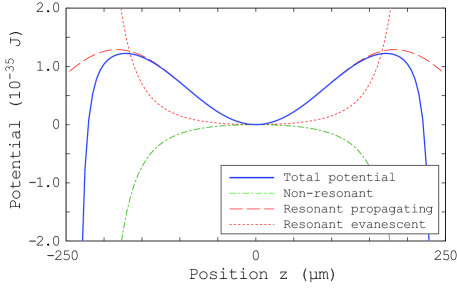
Figure 1: Casimir-Polder potential of a ground-state LiH molecule inside a gold cavity of width $a=500\mu$m at room temperature ($T=300$K). The non-resonant, propagating, and evanescent contributions to the total potential are shown separately.

It is seen that the non-resonant potential is attractive and has a maximum at the center of the cavity, while the evanescent potential is repulsive and has a minimum at the cavity center. As in the case of a single surface ellingsen09 these two contributions partially cancel, where the attractive non-resonant contribution is slightly larger and leads to an attractive total potential in the vicinity of the cavity walls. The propagating part of the potential is spatially oscillating and finite at the cavity walls, it dominates in the central region of the cavity where it gives rise to well-pronounced maxima and minima.

It is natural to wonder whether these potential minima might be used for the purpose of guiding of polar molecules. With this in mind, we will in the following discuss strategies of enhancing the depth of the potential well by analyzing the dependence of the potential on the molecular species as well as the geometric and material parameters of the cavity.

II.1 Cavity-induced enhancement of the potential

We begin our analysis by discussing the dependence of the potential on the cavity width. The one-dimensional confinement of the propagating modes in a cavity of highly reflecting mirrors leads to the formation of standing waves and associated cavity resonances. When the molecular transition frequency coincides with one of these resonances, the thermal CP potential can be strongly enhanced: When the squared reflection coefficient $r_{\sigma}^{2}$ is close to unity, the denominator $D_{\sigma}$ of Eq. (7), featuring in the Green tensor, becomes small if the exponential $\exp(2i\beta a)$ is equal to unity, resulting in a strong enhancement of the potential $U_{\mathrm{pr}}$. This happens for normal incidence ($k_{\perp}=0$) of the propagating waves, when the resonance condition $2\omega_{0k}a/c=2\pi\nu,~{}~{}\nu\in\mathbb{N}$ is fulfilled. In other words, the cavity length has to be equal to a half-integer multiple of the molecular transition wavelength $\lambda_{k0}=2\pi c/\omega_{k0}$:

$$a=\nu\lambda_{k0}/2,~{}~{}\nu\in\mathbb{N}.$$ (14)

We say that the molecular transition coincides with the $\nu$th cavity resonance.

The cavity-induced enhancement of the thermal CP potential is illustrated in Fig. 2, where we show the total thermal CP potential of a ground-state LiH molecule in gold cavities of widths such that the molecular transition is close to the second cavity resonance $\lambda_{k0}$.

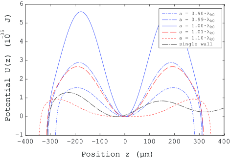
Figure 2: Cavity-induced enhancement of the thermal Casimir-Polder potential of a ground-state LiH molecule inside gold cavities of various widths close to the second resonance $a=\lambda_{k0}=673\mu\mathrm{m}$. The potential of a single plate at $z=-\lambda_{k0}/2$ is also displayed.

As seen, the amplitude of the spatial oscillations, associated with the propagating part of the potential $U_{\mathrm{pr}}$, sharply increases as the cavity width approaches $\lambda_{k0}$. For comparison, we have also displayed the potential of a single plate at $z=-\lambda_{k0}/2$, where Eq. (II) for the cavity Green tensor has been replaced with the single-plate result ellingsen09

$$\operatorname{Tr}\mbox{{{G}}}^{(1)}(\mathbf{r},\mathbf{r}^{\prime},\omega)$$

$$=\frac{i}{4\pi}\int_{0}^{\infty}\frac{k_{\perp}dk_{\perp}}{\beta}\sum_{\sigma=s,p}\biggl{[}r_{\sigma}-2\,\frac{c^{2}\beta^{2}}{\omega^{2}}\,r_{p}\biggr{]}e^{i\beta(a+2z)}.$$ (15)

The comparison shows that the amplitude of the oscillations, while hardly visible for the single plate, is strongly enhanced for a cavity. The depth of the potential minimum at the center of the cavity with respect to the neighboring maxima is increased by a factor 6.7 when using a resonant cavity rather than a single plate.

II.2 Different cavity resonances

In the following, we are interested in the cavity-enhanced oscillations of the thermal potential. As seen from Fig. 2, they set in at some distance away from the cavity walls where the potential is well approximated by its propagating-wave contribution $U_{\mathrm{pr}}$. We can therefore restrict our attention to this part of the total CP potential. The (propagating-wave) potentials associated with different cavity resonances $\nu$ are shown in Fig. 3.

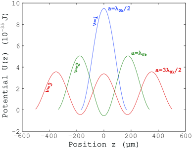
Figure 3: Propagating part of the thermal Casimir-Polder potentials of a ground-state LiH molecule inside gold cavities of widths $a=\nu\lambda_{k0}/2$ corresponding to resonances of different orders ($\nu=1,2,3$).

It is seen that the order $\nu$ of the resonance corresponds to the number of maxima of the potential. Potentials associated with resonances of order $\nu\geq 2$ have minima. The amplitudes of the oscillations become generally smaller for higher resonance orders $\nu$. As seen from the case $\nu=3$, the minima and maxima are slightly more pronounced towards the cavity walls.

The scaling of the potential minima with the resonance order as observed in Fig. 3 can be confirmed by an analytical analysis. For each cavity order $\nu$, we define $\Delta U_{\nu}$ to be the depth of the deepest potential minimum with respect to the neighboring maxima. As suggested by Fig. 3, this deepest minimum will always be the one closest to the cavity walls. Cavity QED problems can often be solved analytically under the simplifying assumption that reflection coefficients are independent of the transverse wave number $k_{\perp}$ ellingsen08 ; ellingsen08e , and this method is also successful here. As shown in App. A, in the perfect conductor limit $r_{p}=-r_{s}\equiv r\to 1$, we have the simple scaling law

$$\Delta U_{\nu}\propto\frac{1}{\nu}\,.$$ (16)

For imperfect conductors, the $\Delta U_{\nu}$ will decrease somewhat less slowly with $\nu$.

The analytical scaling law obtained on the basis of simplifying assumptions supports the observation from the numerical results in Fig. 3 that the $\nu=2$ resonance provides the deepest potential minimum. In view of potential guiding, we can therefore restrict our attention to this case, $\Delta U\equiv\Delta U_{2}$.

II.3 Different molecular species

The CP potential depends on the molecular transition in question via the respective transition frequencies and dipole matrix elements. Using the molecular data as listed in Ref. buhmann08b , we have calculated the depth of the $\nu=2$ potential minimum for both rotational and vibrational transitions of the polar molecules LiH, NH, OH, OD, CaF, BaF, YbF, LiRb, NaRb, KRb, LiCs, NaCs, KCs, and RbCs; the results are displayed in order of descending $\Delta U$ in Fig. 4.

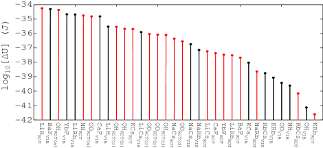
Figure 4: Depth $\Delta U$ of the $\nu=2$ potential minimum for rotational and vibrational transitions of various ground-state polar molecules inside gold cavities at $T=300\mathrm{K}$. The different non-degenerate transitions of OH and OD are labeled as (a)-(d) in order of ascending frequencies, cf. Ref. buhmann08b .

The figure shows that the deepest potential minima are realized when using the rotational transition of LiH, the vibrational transition of BaF or the dominant rotational transition of OH, followed by YbF (vibrational), LiRb (vibrational), NH (rotational), OD (dominant rotational transition), and CaF (vibrational).

The variation in the depth for different molecules is partly due to its dependence on the molecular transition frequency. As shown in Ref. ellingsen09 , the resonant part of the CP potential of a single plate is proportional to $\omega_{k0}^{2}n(\omega_{k0})$ for a good conductor with frequency-independent reflectivities. This remains true in the case of a cavity. In addition, the amplitude of the oscillations is inversely proportional to the molecule-wall separation. The largest potential maximum being situated at $z-a/2=\lambda_{k0}/4\propto 1/\omega_{k0}$, its height carries an additional $\omega_{k0}$-proportionality. The dependence of the potential-minimum depth on molecular transition frequency can thus be given as

$$\Delta U_{\nu}\propto\omega_{k0}^{3}n(\omega_{k0})\propto\begin{cases}\omega_{k0}^{2}\quad\mbox{for }\hbar\omega_{k0}\ll k_{\mathrm{B}}T,\\ e^{-\hbar\omega_{k0}/k_{\mathrm{B}}T}\quad\mbox{for }\hbar\omega_{k0}\gg k_{\mathrm{B}}T\,.\end{cases}$$ (17)

As shown in Sec. II.4, this scaling becomes exact for cavities with frequency- and $k_{\perp}$-independent reflectivities. For real conductors, the decrease of $\Delta U_{\nu}$ for high frequencies will be stronger than given in Eq. (17) due to the decrease of the reflection coefficients. Note that Eq. (17) also shows that $\Delta U_{\nu}$ becomes larger for higher temperatures due to the increased thermal-photon number. Again, this only holds when disregarding the temperature dependence of the reflection coefficients, cf. also Sec. II.5 below.

The frequency-dependence of $\Delta U_{\nu}$ is illustrated in Fig. 5 where we have plotted its values normalized by dividing by the transition dipole moments $d^{2}$ ($d^{2}\equiv\sum_{k}|\mathbf{d}_{0k}|^{2}$).

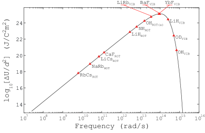
Figure 5: Frequency-dependence of the depth $\Delta U$ of the $\nu=2$ potential minimum for polar molecules inside gold cavities at $T=300\mathrm{K}$.

The transition frequencies of some of the molecules investigated are indicated in the figure. In particular, the vibrational transitions of BaF and YbF, which have been seen in Fig. 4 to give rise to large potential-minimum depths, are very close to the peak of the function $\omega_{k0}^{3}n(\omega_{k0})$, which is at $\omega_{k0}=1.11\times 10^{14}\mathrm{rad}/\mathrm{s}$ for room temperature.

The other main dependence of $\Delta U_{\nu}$ on the molecular species and transition is the proportionality to the modulus squared of the transition-dipole moments,

$$\Delta U_{\nu}\propto\sum_{k}|\mathbf{d}_{0k}|^{2}=d^{2}.$$ (18)

The transition-dipole moments are typically larger for rotational transitions than for vibrational ones. For this reason, the rotational transition of LiH gives rise to the largest minimum depth although the vibrational transition frequencies of BaF and YbF are much closer to the peak frequency $1.11\times 10^{14}\mathrm{rad}/\mathrm{s}$.

II.4 Scaling with reflectivity

The cavity-induced enhancement of the thermal CP force strongly depends on the reflectivity of the cavity walls. To understand this dependence in more detail, let us for simplicity investigate how the height of the single maximum for a $\nu=1$ resonance depends on reflectivity. The scaling of the potential extrema with reflectivity is the same for all $\nu$ as is shown in App. A, so considering the simplest case will suffice.

We begin by writing the propagating part of the resonant CP potential associated with a single transition in the form

$$U_{\mathrm{pr}}(z)=\frac{1}{3\varepsilon_{0}}n(\omega_{k0})|\mathbf{d}_{01}|^{2}I(\phi)$$ (19)

where we have introduced the dimensionless position

$$\phi=\frac{z}{a}$$ (20)

and the integral

$$I(\phi)=\mathrm{Im}\int_{0}^{{\omega_{k0}}/c}\frac{dk_{\perp}k_{\perp}}{2\pi\beta}\Biggl{[}2\beta^{2}\frac{r_{p}}{D_{p}}-\frac{\omega_{k0}^{2}}{c^{2}}\sum_{\sigma=s,p}\frac{r_{\sigma}}{D_{\sigma}}\Biggr{]}\\ \times e^{i\beta a}\cos 2\beta a\phi.$$ (21)

As in Sec. II.2, we consider the simple model case of frequency- and $k_{\perp}$-independent reflection coefficients $r_{p}=-r_{s}\equiv r$. With this assumption,

$$\sum_{\sigma=s,p}\frac{r_{\sigma}}{D_{\sigma}}=0.$$ (22)

After introducing the dimensionless integration variable $x=2\beta a$ with $k_{\perp}dk_{\perp}=-4a^{2}xdx$, the integral above takes the form

$$I(\phi)=\frac{r}{8\pi a^{3}}\,\mathrm{Im}\int_{0}^{x_{0}}dx\,\frac{x^{2}e^{ix/2}\cos\phi x}{1-r^{2}e^{ix}}$$ (23)

where $x_{0}=2\omega_{k0}a/c$. For the $\nu=1$ resonance, we have $a=\lambda_{0k}/2=\pi c/\omega_{k0}$, so $x_{0}=2\pi$.

The required height of the potential maximum at the cavity center ($z=0$) with respect to the value of $U_{\mathrm{pr}}$ at the cavity walls $z=\pm a/2$ is proportional to the difference $I(0)-I(\frac{1}{2})$. We have

$$I(1/2)= \;\frac{r}{16\pi a^{3}}\,\mathrm{Im}\int_{0}^{2\pi}dxx^{2}\,\frac{e^{ix}+1}{1-r^{2}e^{ix}}$$

$$= \;\frac{r}{16\pi a^{3}}\,\mathrm{Im}\int_{0}^{2\pi}dxx^{2}\left[1+(1+r^{-2})\operatorname{Li}_{0}(r^{2}e^{ix})\right]$$ (24)

where the polylogarithmic function is defined as

$$\operatorname{Li}_{s}(z)=\sum_{k=1}^{\infty}\frac{z^{k}}{k^{s}}.$$ (25)

The first term in Eq. (24) is real and does not contribute. The second one is easily calculated using the relation

$$\int dz\operatorname{Li}_{s}(Ae^{bz})=\frac{1}{b}\operatorname{Li}_{s+1}(Ae^{bz})+C$$ (26)

valid for arbitrary constants $A,b$ where $|A|<1$. Partially integrating this relation twice and substituting the result for $A=r^{2}$, $b=i$ into Eq. (24), one finds

$$I(1/2)= \frac{r+r^{-1}}{16\pi a^{3}}\,\mathrm{Im}\left\{\frac{4\pi^{2}}{i}\operatorname{Li}_{1}(r^{2})+4\pi\operatorname{Li}_{2}(r^{2})\right\}$$

$$= \frac{\pi(r+r^{-1})}{4a^{3}}\,\ln(1-r^{2}),$$ (27)

where we have noted that $\operatorname{Li}_{1}(z)=-\ln(1-z)$. In the limit of high reflectivity, $\delta\equiv 1-r\to 0_{+}$ this exact result shows the asymptotic behavior

$$I(1/2)\sim\frac{\pi}{2a^{3}}(\ln\delta+\ln 2)\quad\mbox{for }\delta\to 0_{+},$$ (28)

with the first correction term being of order $\delta$.

The calculation of $I(0)$ is only slightly more involved. We have

$$I(0)= \frac{r}{8\pi a^{3}}\,\mathrm{Im}\int_{0}^{2\pi}dx\frac{x^{2}e^{ix/2}}{1-r^{2}e^{ix}}$$

$$= \frac{r}{8\pi a^{3}}\,\sum_{l=0}^{\infty}r^{2k}\mathrm{Im}\int_{0}^{2\pi}dxx^{2}e^{ix(l+\frac{1}{2})}.$$ (29)

By partial integration we obtain

$$\mathrm{Im}\int_{0}^{2\pi}dx\,x^{2}e^{ix(l+\frac{1}{2})}=\frac{4\pi^{2}}{(l+\frac{1}{2})}-\frac{4}{(l+\frac{1}{2})^{3}}.$$ (30)

After substitution of this result, the sum over $l$ can be performed by using the relations (cf. §1.513 in Ref. BookGradshteyn80 )

$$\sum_{l=0}^{\infty}\frac{r^{2l}}{l+\frac{1}{2}}=\frac{1}{r}\ln\frac{1+r}{1-r}\sim-\ln\delta+\ln 2\quad\mbox{for }\delta\to 0_{+}$$ (31)

(leading corrections being of the order $\delta\ln\delta$) and

$$\sum_{l=0}^{\infty}\frac{r^{2l}}{(l+\frac{1}{2})^{3}}\\ \sim 8\left[\sum_{l=1}^{\infty}\frac{1}{l^{3}}-\sum_{l=1}^{\infty}\frac{1}{(2l)^{3}}\right]=7\zeta(3)\quad\mbox{for }\delta\to 0_{+},$$ (32)

where $\zeta(z)$ is the Riemann zeta function. We thus find

$$I(0)\sim-\frac{\pi}{2a^{3}}[\ln\delta-\ln 2+\frac{7}{\pi^{2}}\zeta(3)]\quad\mbox{for }\delta\to 0_{+},$$ (33)

with the first correction again being of order $\delta\ln\delta$.

Substituting the results (28) and (33) into Eq. (19), the difference between the maximum and minimum values of the $\nu=1$ propagating potential reads

$$U_{\mathrm{pr}}(0)-U_{\mathrm{pr}}(a/2)\sim-\frac{\pi\sum_{k}|\mathbf{d}_{0k}|^{2}n(\omega_{k0})}{3\varepsilon_{0}a^{3}}\left[\ln\delta\!+\!\frac{7\zeta(3)}{2\pi^{2}}\right]$$

$$\quad\mbox{for }\delta\to 0_{+}.$$ (34)

This result being representative of the case of arbitrary $\nu$, we can conclude that

$$\Delta U_{\nu}\propto\ln(1-r)$$ (35)

in the limit $r\to 1$. In the case where the reflection coefficients are not the same for both polarizations but still assumed constant, the coefficient of the term $\propto\ln\delta$ in Eq. (II.4) will change, leading to a slight quantitative but no qualitative difference to the scaling of the potential-minimum depth. Note that Eq. (II.4) immediately implies the scaling law (17) for the frequency dependence of $\Delta U_{\nu}$.

The fact that the potential depth diverges only logarithmically as reflectivity tends to unity poses severe restrictions on the potential which is obtainable using a planar cavity. The mathematical reason for the relative weakness of the resonance is that the integrand of the $k_{\perp}$-integral only becomes large at a single point, at $k_{\perp}=0$. The physical reason is that the photonic modes in the cavity are only confined in one out of three spatial dimensions. We conjecture that the potential due to the resonant CP force on a ground state molecule can be much increased by a resonant cavity if confinement is imposed in two or even three dimensions, i.e. in a cylindrical or spherical cavity.

The logarithmic scaling law of the potential-minimum depth $\Delta U_{\nu}$ for the case $\nu=2$ is confirmed by a numerical calculation in which reflection coefficients are set constant, $r_{p}=-r_{s}\equiv r$ and close to unity.

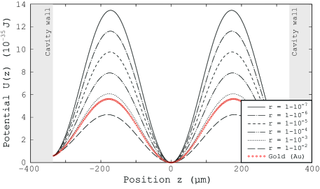
Figure 6: Propagating part of the thermal CP potential for a ground-state LiH molecule inside different cavities with constant reflection coefficients. The rotational transition of LiH is assumed to coincide with the $\nu=2$ resonance of the cavities. For comparison, the exact result for a gold cavity is also shown.

The result for the rotational transition of LiH is shown in Fig. 6 where the exact result for a gold cavity is also included. By comparing the latter curve to the potentials for constant reflection coefficients, one can read off the relatively small ‘effective’ reflectivity of gold between $1-10^{-2}$ and $1-10^{-3}$ at the respective transition frequency of LiH. For a molecule with a smaller eigenfrequency $\omega_{k0}$ the gold cavity does slightly better because the permittivity is larger. Consider the vibrational transition of YbF with $\omega_{k0}\approx 9\cdot 10^{10}$rad/s as an example, for which the ‘effective’ reflectivity of the gold cavity (in the sense of figure 6) increases to about $1-10^{-3.5}$.

II.5 Enhanced reflectivity using Bragg mirrors

In contrast with the non-resonant CP force which depends on a very broad band of frequencies, the resonant part of the ground state force on a two-level molecule depends on the reflection properties of the cavity at a single frequency, $\omega=\omega_{k0}$. In addition, the resonance of the cavity is also associated with a single value of the wave vector $\mathbf{k}_{\perp}$, namely normal incidence. An enhancement of the propagating potential hence does not require a good conductor like gold which is a good reflector for a broad range of frequencies and all angles of incidence; instead, cavity walls whose reflectivity has a sharp peak at normal incidence and the single frequency $\omega_{k0}$ are sufficient. The obvious candidate is to use multilayer Bragg mirrors, which consist of alternating layers of two different materials, each layer of thickness being equal to one quarter of the wavelength $\lambda_{10}=2\pi/n\omega_{k0}$ in that layer where $n$ is the respective refractive index.

The reflection coefficient of a stack of layers with permittivities $\varepsilon_{j}$ and thicknesses $d_{j}$ is found by recursive use of the formula

$$r_{ijk\cdots}=\frac{r_{ij}+r_{jk(l\cdots)}e^{2i\beta_{j}d_{j}}}{1+r_{ij}r_{jk(l\cdots)}e^{2i\beta_{j}d_{j}}}$$ (36)

($\beta_{j}=\sqrt{n_{j}^{2}\omega^{2}/c^{2}-k_{\perp}^{2}}$), which relates the reflection coefficient of a set of three adjacent layers $ijk\cdots$ (and all the layers behind) to the respective result for the next set of adjacent layers $jkl\cdots$. If the $k$th layer is the last one of the stack, the coefficients $r_{jk(l\cdots)}$ reduce to the two-layer coefficients $r_{jk}$. In straightforward generalization of Eqs. (9a) and (9b), the two-layer coefficients read

$$r_{ij}^{s}= \frac{\beta_{i}-\beta_{j}}{\beta_{i}+\beta_{j}}\,;$$ (37a)

$$r_{ij}^{p}= \frac{\varepsilon_{j}\beta_{i}-\varepsilon_{i}\beta_{j}}{\varepsilon_{j}\beta_{i}+\varepsilon_{i}\beta_{j}}\;,$$ (37b)

for $s$- and $p$-polarized waves, respectively. The Casimir effect for such multilayer stacks has been extensively studied in the past esquivel-sirvent01 ; raabe03 ; tomas05 ; ellingsen07 .

A very common pair of materials to use for Bragg mirrors is GaAs and AlAs. At the rotational transition frequency of LiH, the permittivity of the two materials can be roughly given as $\varepsilon_{\text{GaAs}}=12.96+0.02i$ johnson69 ; courtney77 and $\varepsilon_{\text{AlAs}}=10.96+0.02i$ adachi85 . The reflection coefficient of a GaAs/AlAs Bragg mirror is plotted as a function of the number of (double) layers $N$ in the upper panel of Fig. 7. For a given $N$, the Bragg mirror consists of $2N+1$ layers in total, i.e. $N$ pairs of GaAs and AlAs layers of thickness $\lambda_{10}/4$ (beginning with GaAs) and a terminating GaAs layer of infinite thickness.

Figure 7: Reflection coefficients of Bragg mirrors for normal incidence at the rotational transition frequency of LiH vs the number of double layers $N$. Above: GaAs/AlAs mirror, where the results for reduced and vanishing absorption are also displayed for comparison. Below: Vacuum/sapphire mirror at two different temperatures $T=77$K and $300$K.

As Fig. 7 shows, the reflectivity initially increases for increasing $N$ and then eventually saturates for $N\gtrsim 30$ to some finite value where $1-\mathrm{Re}\,r\simeq 10^{-2}$. This saturation is due to absorption, as is illustrated by the other two curves, where we have given the results that would be obtained for a reduced or vanishing imaginary part of the permittivities. For a reduced imaginary part, the saturation sets in for higher $N$, and consequently to a lower $\delta$. In the absence of absorption, the reflectivity could be brought arbitrarily close to unity by adding more and more layers.

A higher reflectivity could hence be obtained by using materials with very small dielectric loss. One example of such a Bragg mirror could be alternating layers of vacuum and sapphire, which can have an extremely low loss tangent ($\mathrm{Im}\,\varepsilon/\mathrm{Re}\,\varepsilon\simeq 10^{-5}$ and $10^{-7}$ at room temperature and $77$K, respectively driscoll92 ) combined with a refractive index considerably larger than unity ($\mathrm{Re}\,\varepsilon\simeq 10$ wang08 ). Using the approximative values $\varepsilon_{\text{sapph}}=10+10^{-4}i$ at $300$K and $\varepsilon_{\text{sapph}}=10+10^{-6}i$ at $77$K, we have computed the reflection coefficients of the vacuum/sapphire mirror as displayed in the lower panel of Fig. 7. At room temperature, the coefficient saturates at $N\gtrsim 6$ to $\delta=5.5\cdot 10^{-6}$. At $T=77$K, the reflection coefficient saturates at $N\gtrsim 8$ to $\delta=5.5\cdot 10^{-8}$, the the increase in reflectivity is obviously due to the reduction of material absorption for the lower temperature. Note that in comparison to the GaAs/AlAs mirror, the number of layers required for saturation is significantly lower because of the larger dielectric contrast; and the room-temperature reflectivity at saturation is increased by about four orders of magnitude.

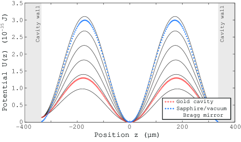
Figure 8: Resonant part of the thermal CP potential associated with the rotational transitions of a ground-state LiH molecule at $\nu=2$ resonance with a gold cavity and a cavity bounded by vacuum/sapphire Bragg mirrors at two different temperatures: $77$K above, $300$K below. The solid black lines represent calculations at constant reflection coefficients as in Fig. 6; the corresponding values of $1-r$ decrease in powers of $10$ from $10^{-2}$ (lowest curve) to $10^{-7}$ (highest curve). The same permittivity is used for gold for both temperatures.

The resulting propagating part of the resonant CP potential at resonant cavity width using the sapphire/vacuum Bragg mirror at $T=77$K and $300$K are shown in Fig. 8, where the corresponding graphs at various constant reflection coefficients have also been displayed for reference. The ‘effective’ reflection coefficients achieved at the two temperatures are around $\delta=10^{-4.8}$ and $\delta=10^{-6.7}$ respectively, and the potential depths approximately a factor $2.45$ and $1.77$ greater than that of the gold cavity at the same temperatures. Note, however, that the effect of the enhanced reflectivity at $77$K is counteracted by the overall decrease of the potential due to the lower photon number.

II.6 Lifetime of the ground state in the cavity

Resonant CP potentials are only present for molecules which are not at equilibrium with their thermal environment, i.e., on a time scale given by the inverse heating rate ellingsen09 . When enhancing the thermal CP potential via a resonant cavity, it is necessary to ascertain that the simultaneous cavity-enhancement of heating rates does not reduce the lifetime of the resonant potential by so much as to render it experimentally inaccessible. We show in the following that the lifetime of the molecular ground state is not radically changed even by the presence of a resonant planar cavity.

The total heating rate of an isotropic molecule out of its ground state may be written as buhmann08 $\Gamma=\Gamma_{0}+\Gamma_{\text{cav}}$ where

$$\Gamma_{0}=\frac{\sum_{k}|\mathbf{d}_{0k}|^{2}\omega_{k0}^{3}n(\omega_{k0})}{3\pi\hbar c^{3}\varepsilon_{0}}$$ (38)

is the heating rate in free space and

$$\Gamma_{\text{cav}}=\frac{2\mu_{0}}{3\hbar}\sum_{k}|\mathbf{d}_{0k}|^{2}\omega_{k0}^{2}n(\omega_{k0})\mathrm{Im}\operatorname{Tr}\mbox{{{G}}}^{(1)}(\mathbf{r},\mathbf{r},\omega_{k0})$$ (39)

is its change due to the presence of the cavity. Apart from the prefactor, this additional term has the same form as the expression for the potential, except that the imaginary part of the Green tensor is taken rather than the real part.

In Sec. II.4, we had shown that for real and constant reflection coefficients, the Green tensor exhibits a logarithmic divergence as $r\to 1$ with a purely real coefficient, whereas all other contributions remain finite. This shows that the imaginary part of the Green tensor responsible for the decay rate can be expected to remain finite even for strongly increased reflectivity. It follows that the presence of the cavity does not drastically change the lifetime of the ground state of the molecule, which will typically be in the order of seconds. This is confirmed in Fig. 9 where we display the ground-state heating rate of a LiH molecule inside a $\nu=1$ gold cavity and near a gold half-space. The lifetime is reduced by only a factor 2 at the center of the cavity, remaining in the order of seconds.

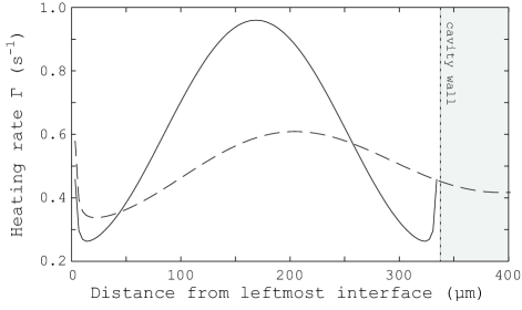
Figure 9: Ground-state rotational heating rate of a LiH molecule in a gold cavity at $\nu=1$ resonance $a=\pi c/\omega_{k0}$ (solid line) and to the right of a gold half-space (dashed line) at room temperature ($T=300$K).

III Conclusions and outlook

We have studied the thermal Casimir-Polder potential of ground-state polar molecules placed within a planar cavity at room temperature. As was previously found in Ref. ellingsen09 , the resonant absorption of thermal photons by a molecule gives rise to spatial oscillations of that potential. Our results demonstrate that the amplitude of these oscillations is enhanced when placing the molecule inside a suitable cavity such that a molecular transition frequency coincides with a cavity resonance. We have analyzed the dependence of this oscillating potential on the parameters of the molecule and the cavity by both analytical and numerical means and found that the depth of potential minima $\ldots$

• Cavity resonance: $\ldots$ decreases with increasing order of the cavity resonance approximately as $1/\nu$;

• Molecular eigenfrequency: $\ldots$ is proportional to $\omega_{k0}^{3}n(\omega_{k0})$ for good conductors, where $n(\omega_{k0})$ is the thermal photon number;

• Molecular dipole moments: $\ldots$ is proportional to the modulus squared $\sum_{k}|\mathbf{d}_{0k}|^{2}=d^{2}$ of the total transition dipole moment;

• Temperature: $\ldots$ increases with temperature due to an increase of the thermal photon number $n(\omega_{k0})$;

• Reflectivity of cavity walls: $\ldots$ scales as $\ln(1-r)$ for high reflectivity $r$.

In view of observing this potential and possibly utilizing it for the guiding of cold polar molecules, these observations imply the following strategies for enhancing the depth of the potential minima:

• Cavity resonance: The $\nu=2$ resonance is most suitable, since it gives the deepest minimum.

• Molecular species: At room temperature, the deepest minima are realized for molecules whose transitions are not too far from the peak frequency $1.11\times 10^{14}\mathrm{rad}/\mathrm{s}$ and which at the same time feature suitably large transition dipole moments. Good candidates are, e.g., LiH (rotational transitions), BaF (vibrational transitions) or OH (rotational transitions).

• Cavity walls: Highly reflecting cavities are required in order to enhance the potential. Bragg mirrors consisting of materials with small absorption such as sapphire are favorable to single layers of good conductors like gold.

• Temperature: Temperatures should be in the range of room temperature or even higher in order to achieve large photon numbers. This should be balanced, however, against the adverse reduction of reflectivity of most materials with increasing temperature.

With an optimum choice of all these parameters, the planar cavity can be used to enhance the resonant potential by one or at most two orders of magnitude with respect to the single-plate case. However, the thermal potentials achievable with planar cavities are in all likelihood still too small to facilitate the guiding of polar molecules.

The limitations of the enhancement of the potential in a planar cavity are ultimately due to the weak (logarithmic) scaling with reflectivity. A stronger scaling may be expected in geometries providing mode confinement in more than just one dimension such as cylindrical or spherical cavities. This will be investigated in a future publication. Note that apart from the different expected scaling with reflectivity, all other conclusions regarding the dependence of the potential on the relevant molecular and material parameters as given above hold irrespective of the geometry under consideration. The strategies for the enhancement of thermal CP potentials developed in this work will thus present a valuable basis when considering more complicated cavity geometries.

Appendix A Scaling of potential depth with resonance order

For a cavity of width $a=\nu\lambda_{k0}/2$ the potential has $\nu$ peaks, roughly located at $z=-\nu\lambda_{k0}/4+(\mu-1/2)\lambda_{k0}/2$ ($\mu=1\ldots\nu$) and $\nu-1$ minima at $z=-\nu\lambda_{k0}/4+\mu\lambda_{k0}/2$ ($\mu=1\ldots\nu-1$). For a given resonance order $\nu$, the deepest minima are the ones closest to the cavity walls (and which have a maximum on both sides), for example the rightmost one at $z=(\nu-2)\lambda_{k0}/4$. It has to be compared with the lower of the two adjacent maxima, i.e., the one immediately to the right at $z=(\nu-3)\lambda_{k0}/4$. The required depth of the deepest minimum is hence given by

$$\Delta U_{\nu}=U[(\nu-3)\lambda_{k0}/4]-U[(\nu-2)\lambda_{k0}/4].$$ (40)

We calculate this depth for a cavity whose reflection coefficients are independent of the transverse wave number $k_{\perp}$, $r_{p}=-r_{s}\equiv r$, and close to unity, $\delta=1-r\ll 1$. Noting that the oscillating part of the potential is determined by $U_{\mathrm{pr}}$ and introducing the definition (21), cf. Sec. II.4, we thus have

$$\Delta U_{\nu}\propto I\bigl{(}{\textstyle\frac{1}{2}-\frac{3}{2\nu}}\bigr{)}-I\bigl{(}{\textstyle\frac{1}{2}-\frac{1}{\nu}}\bigr{)}.$$ (41)

We consider in the following only the terms which do not vanish as $\delta\to 0_{+}$. For arbitrary $\phi$, we have

$$I(\phi)=\frac{r}{2\pi\nu^{3}\lambda_{0k}^{3}}\mathrm{Im}\int_{0}^{2\pi\nu}dx\frac{x^{2}e^{ix/2}\cos\phi x}{1-r^{2}e^{ix}}$$ (42)

which, after expanding the fraction in powers of $r^{2}$, solving the integral over $x$ and taking the imaginary part, can be written as

$$I(\phi)=\frac{r}{2\pi\nu^{3}\lambda_{0k}^{3}}\sum_{j=0}^{\infty}\left[y(j+\tfrac{1}{2}+\phi)+y(j+\tfrac{1}{2}-\phi)\right]$$ (43)

with

$$y(p)= -\frac{2}{p^{3}}+\left(\frac{2}{p^{3}}-\frac{4\nu^{2}\pi^{2}}{p}\right)\cos(2\pi\nu p)$$

$$+\frac{4\nu\pi}{p^{2}}\sin(2\pi\nu p).$$ (44)

In particular, this implies

$$I(\textstyle\frac{1}{2}-\textstyle\frac{3}{2\nu})= \frac{2r}{\pi\nu^{3}\lambda_{0k}^{3}}\sum_{j=0}^{\infty}r^{2j}\left[\frac{\nu^{2}\pi^{2}}{j+1-\textstyle\frac{3}{2\nu}}+\frac{\nu^{2}\pi^{2}}{j+\textstyle\frac{3}{2\nu}}\right.$$

$$\left.-\frac{1}{(j+1-\textstyle\frac{3}{2\nu})^{3}}-\frac{1}{(j+\textstyle\frac{3}{2\nu})^{3}}\right],$$ (45a)

$$I(\textstyle\frac{1}{2}-\textstyle\frac{1}{\nu})= -\frac{2r\pi}{\nu\lambda_{0k}^{3}}\sum_{j=0}^{\infty}\left[\frac{r^{2j}}{j+1-\textstyle\frac{1}{\nu}}+\frac{r^{2j}}{j+\textstyle\frac{1}{\nu}}\right]$$ (45b)

The evaluation of sums with simple denominators can be performed by using the relation (formula 9.559 in Ref. BookGradshteyn80 )

$$\sum_{j=0}^{\infty}\frac{r^{2j}}{j+b}=\frac{1}{b}F(1,b;1+b;r^{2}),$$ (46)

valid for any $b\neq 0,-1,-2,...$ Here, $F(a,b;c;z)\equiv{}_{2}F_{1}(a,b;c;z)$ is a hypergeometric function which in turn has the following expansion in powers of $\delta=1-r$ (formula 15.3.10 in Ref. BookAbramowitz64 )

$$\frac{1}{b}F(1,b;1+b;r^{2})\sim -\ln\delta-\ln 2-\gamma-\psi(b)$$ (47)

as $\delta\to 0_{+}$, the correction terms being of order $\delta\ln\delta$. Here, $\psi(x)$ is the logarithmic derivative of the gamma function and $\psi(1)=-\gamma$ where $\gamma=0.577216$ is Euler’s constant.

For the sums in Eq. (45) with cubic denominators, one can set $r=1$ with an error of order $\delta$. The sums are then simply Hurwitz zeta functions $\zeta(3,b)$

$$\sum_{l=0}^{\infty}\frac{1}{(l+b)^{3}}\equiv \zeta(3,b).$$ (48)

We thus find

$$I\bigl{(}{\textstyle\frac{1}{2}-\frac{3}{2\nu}}\bigr{)}-I\bigl{(}{\textstyle\frac{1}{2}-\frac{1}{\nu}}\bigr{)}=-\frac{8\pi}{\nu\lambda_{0k}^{3}}[\ln\delta+\varphi(\nu)]+...$$ (49)

as $\delta\to 0_{+}$ with corrections being of order $\delta\ln\delta$ and

$$\varphi(\nu)\equiv \ln 2+\gamma+\textstyle\frac{1}{4}\psi(1-\textstyle\frac{3}{2\nu})+\textstyle\frac{1}{4}\psi(\textstyle\frac{3}{2\nu})$$

$$+\textstyle\frac{1}{4}\psi(1-\textstyle\frac{1}{\nu})+\textstyle\frac{1}{4}\psi(\textstyle\frac{1}{\nu})$$

$$+\frac{1}{4\pi^{2}\nu^{2}}\left[\zeta(3,1-\textstyle\frac{3}{2\nu})+\zeta(3,\textstyle\frac{3}{2\nu})\right].$$ (50)

Some numerical values of $\varphi(\nu)$ are

$$\varphi(2)= -0.1134423724;$$ (51a)

$$\varphi(3)= -0.4015949503;$$ (51b)

$$\varphi(4)= -0.7384479470.$$ (51c)

We give a plot of $\varphi(\nu)/\nu$ in Fig. 10.

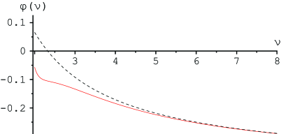
Figure 10: Graph of $\varphi(\nu)/\nu$ (solid, red line) and its asymptote (dashed line) as given by Eq. (52).

For large $\nu$, one obviously has

$$\varphi(j)\sim -(\textstyle\frac{5}{12}-\frac{2}{27\pi^{2}})\nu+\ln(2)+\frac{1}{4}+...$$

$$\approx -0.4091613938j+0.9431471806+...$$ (52)

plus terms of order $\nu^{-1}$ and smaller. Already at $\nu=4$ this is a fairly good approximation to Eq. (A) as shown in Fig. 10.

References

- (1) H.B.G. Casimir and D. Polder, Phys. Rev. 73, 360 (1948).
- (2) E.M. Lifshitz, Zh. Eksp. Teor. Fiz. 29, 94 (1955) [Sov. Phys. JETP 2, 73 (1956)].
- (3) A.D. McLachlan, Proc. R. Soc. Lond. Ser. A 274, 80 (1963).
- (4) C. Henkel, K. Joulain, J.P. Mulet, and J.-J. Greffet, J. Opt. A: Pure Appl. Opt. 4, S109 (2002).
- (5) G.L. Klimchitskaya, E.V. Blagov, and V.M. Mostepanenko, J. Phys. A: Math. Gen. 39, 6481 (2006).
- (6) E.V. Blagov, G.L. Klimchitskaya, and V.M. Mostepanenko, Phys. Rev. B 71, 235401 (2005).
- (7) M. Bordag, B. Geyer, G.L. Klimchitskaya, and V.M. Mostepanenko, Phys. Rev. B 74, 205431 (2006).
- (8) M. Boström and B.E. Sernelius, Phys. Rev. A 61, 052703 (2000).
- (9) V.M. Nabutovskiĭ, V.R. Belosludov, and A.M. Korotkikh, Sov. Phys. JETP 50, 352, (1979).
- (10) E.V. Blagov, G.L. Klimchitskaya, and V.M. Mostepanenko, Phys. Rev. B 75, 235413 (2007).
- (11) M. Antezza, L.P. Pitaevskii, and S. Stringari, Phys. Rev. Lett. 95, 113202 (2005).
- (12) J.M. Obrecht, R.J. Wild, M. Antezza, L.P. Pitaevskii, S. Stringari, and E.A. Cornell, Phys. Rev. Lett. 98, 063201 (2007).
- (13) T. Nakajima, P. Lambropoulos, and H. Walther, Phys. Rev. A 56, 5100 (1997).
- (14) S.-T. Wu and C. Eberlein, Proc. R. Soc. Lond. Ser. A 456, 1931 (2000).
- (15) S.Y. Buhmann and D.-G. Welsch, Prog. Quantum Electron. 31, 51 (2007).
- (16) S. Scheel and S.Y. Buhmann, Acta Phys. Slov. 58, 675 (2008).
- (17) S.Y. Buhmann and S. Scheel, Phys. Rev. Lett. 100, 253201 (2008).
- (18) M.-P. Gorza and M. Ducloy, Eur. Phys. J. D 40 343 (2006).
- (19) S.Å. Ellingsen, S.Y. Buhmann, and S. Scheel, Phys. Rev. A 79, 052903 (2009).
- (20) S.Y.T. van de Meerakker, H.L. Bethlem, and G. Meijer, Nature Physics 4, 595 (2008).
- (21) S.Y. Buhmann, M.R. Tarbutt, S. Scheel, and E.A. Hinds, Phys. Rev. A 78, 052901 (2008).
- (22) G. Barton, Proc. R. Soc. Lond. Ser. A 320, 251 (1970).
- (23) G. Barton, Proc. R. Soc. Lond. Ser. A 367, 117, (1979).
- (24) G. Barton, Proc. R. Soc. Lond. Ser. A 410, 141, (1987).
- (25) W. Jhe, Phys. Rev. A 43, 5795 (1991).
- (26) W. Jhe, Phys. Rev. A 44, 5932 (1991).
- (27) E.A. Hinds, Adv. At. Mol. Opt. Phys. 28, 237 (1991).
- (28) E.A. Hinds, Adv. At. Mol. Opt. Phys. Suppl. 2, 1 (1994).
- (29) M.S. Tomaš, Phys. Rev. A 51, 2545 (1995).
- (30) A. Lambrecht and S. Reynaud, Eur. Phys. J. D 8, 309 (2000).
- (31) S.Å. Ellingsen, Europhys. Lett. 82, 53001 (2008).
- (32) S.Å. Ellingsen, in The Casimir Effect and Cosmology: A volume in honour of Professor Iver H. Brevik on the occasion of his 70th birthday S. Odintsov et al. (eds.) (Tomsk State Pedagogical University Press, 2008), p.45, preprint quant-ph/0811.4214.
- (33) I.S. Gradshteyn and I.M. Ryzhik, Table of Integrals, Series and Products 4th ed. (Academic Press, New York, 1980).
- (34) R. Esquivel-Sirvent, C. Villarreal, and G.H. Cocoletzi, Phys. Rev. A 64, 052108 (2001).
- (35) C. Raabe, L. Knöll, and D.-G. Welsch, Phys. Rev. A 68, 033810 (2003).
- (36) M.S. Tomaš, Phys. Lett. A 342, 381 (2005).
- (37) S.Å. Ellingsen, J. Phys. A 40, 1951 (2007).
- (38) C.J. Johnson, G.H. Sherman, and R. Weil, Appl. Opt. 8, 1667 (1969).
- (39) W.E. Courtney, IEEE Trans. Microwave Th. Tech. 25, 697 (1977).
- (40) S. Adachi, J. Appl. Phys. 58, R1 (1985).
- (41) M.M. Driscoll, J.T. Haynes, R.A. Jelen, R.W. Weinert, J.R. Gavaler, J. Talvacchio, G.R. Wagner, K.A. Zaki, and X.P. Liang, IEEE Trans. Ultrason. Ferroelec. Freq. Contr. 39, 405 (1992).
- (42) G.G. Wang, M.F. Zhang, J.C. Han, X.D. He, H.B. Zuo, and X.H. Yang, Cryst. Res. Technol. 43, 531 (2008).
- (43) M. Abramowitz and I.A. Stegun, Handbook of Mathematical Functions (Dover, New York, 1964).