Rank-Sparsity Incoherence for Matrix Decomposition

Abstract

Suppose we are given a matrix that is formed by adding an unknown sparse matrix to an unknown low-rank matrix. Our goal is to decompose the given matrix into its sparse and low-rank components. Such a problem arises in a number of applications in model and system identification, and is NP-hard in general. In this paper we consider a convex optimization formulation to splitting the specified matrix into its components, by minimizing a linear combination of the $\ell_{1}$ norm and the nuclear norm of the components. We develop a notion of rank-sparsity incoherence, expressed as an uncertainty principle between the sparsity pattern of a matrix and its row and column spaces, and use it to characterize both fundamental identifiability as well as (deterministic) sufficient conditions for exact recovery. Our analysis is geometric in nature, with the tangent spaces to the algebraic varieties of sparse and low-rank matrices playing a prominent role. When the sparse and low-rank matrices are drawn from certain natural random ensembles, we show that the sufficient conditions for exact recovery are satisfied with high probability. We conclude with simulation results on synthetic matrix decomposition problems.

1 Introduction

Complex systems and models arise in a variety of problems in science and engineering. In many applications such complex systems and models are often composed of multiple simpler systems and models. Therefore, in order to better understand the behavior and properties of a complex system a natural approach is to decompose the system into its simpler components. In this paper we consider matrix representations of systems and statistical models in which our matrices are formed by adding together sparse and low-rank matrices. We study the problem of recovering the sparse and low-rank components given no prior knowledge about the sparsity pattern of the sparse matrix, or the rank of the low-rank matrix. We propose a tractable convex program to recover these components, and provide sufficient conditions under which our procedure recovers the sparse and low-rank matrices exactly.

Such a decomposition problem arises in a number of settings, with the sparse and low-rank matrices having different interpretations depending on the application. In a statistical model selection setting, the sparse matrix can correspond to a Gaussian graphical model [18] and the low-rank matrix can summarize the effect of latent, unobserved variables. Decomposing a given model into these simpler components is useful for developing efficient estimation and inference algorithms. In computational complexity, the notion of matrix rigidity [27] captures the smallest number of entries of a matrix that must be changed in order to reduce the rank of the matrix below a specified level (the changes can be of arbitrary magnitude). Bounds on the rigidity of a matrix have several implications in complexity theory [19]. Similarly, in a system identification setting the low-rank matrix represents a system with a small model order while the sparse matrix represents a system with a sparse impulse response. Decomposing a system into such simpler components can be used to provide a simpler, more efficient description.

1.1 Our results

Formally the decomposition problem we are interested can be defined as follows:

Problem

Given $C=A^{\star}+B^{\star}$ where $A^{\star}$ is an unknown sparse matrix and $B^{\star}$ is an unknown low-rank matrix, recover $A^{\star}$ and $B^{\star}$ from $C$ using no additional information on the sparsity pattern and/or the rank of the components.

In the absence of any further assumptions, this decomposition problem is fundamentally ill-posed. Indeed, there are a number of scenarios in which a unique splitting of $C$ into “low-rank” and “sparse” parts may not exist; for example, the low-rank matrix may itself be very sparse leading to identifiability issues. In order to characterize when such a decomposition is possible we develop a notion of rank-sparsity incoherence, an uncertainty principle between the sparsity pattern of a matrix and its row/column spaces. This condition is based on quantities involving the tangent spaces to the algebraic variety of sparse matrices and the algebraic variety of low-rank matrices [16].

Two natural identifiability problems may arise. The first one occurs if the low-rank matrix itself is very sparse. In order to avoid such a problem we impose certain conditions on the row/column spaces of the low-rank matrix. Specifically, for a matrix $M$ let $T(M)$ be the tangent space at $M$ with respect to the variety of all matrices with rank less than or equal to $\mathrm{rank}(M)$. Operationally, $T(M)$ is the span of all matrices with row-space contained in the row-space of $M$ or with column-space contained in the column-space of $M$; see (6) for a formal characterization. Let $\xi(M)$ be defined as follows:

$$\xi(M)\triangleq\max_{N\in T(M),~{}\|N\|\leq 1}\|N\|_{\infty}.$$ (1)

Here $\|\cdot\|$ is the spectral norm (i.e., the largest singular value), and $\|\cdot\|_{\infty}$ denotes the largest entry in magnitude. Thus $\xi(M)$ being small implies that (appropriately scaled) elements of the tangent space $T(M)$ are “diffuse”, i.e., these elements are not too sparse; as a result $M$ cannot be very sparse. As shown in Proposition 4 (see Section 4.3) a low-rank matrix $M$ with row/column spaces that are not closely aligned with the coordinate axes has small $\xi(M)$.

The other identifiability problem may arise if the sparse matrix has all its support concentrated in one column; the entries in this column could negate the entries of the corresponding low-rank matrix, thus leaving the rank and the column space of the low-rank matrix unchanged. To avoid such a situation, we impose conditions on the sparsity pattern of the sparse matrix so that its support is not too concentrated in any row/column. For a matrix $M$ let $\Omega(M)$ be the tangent space at $M$ with respect to the variety of all matrices with number of non-zero entries less than or equal to $|\mathrm{support}(M)|$. The space $\Omega(M)$ is simply the set of all matrices that have support contained within the support of $M$; see (8). Let $\mu(M)$ be defined as follows:

$$\mu(M)\triangleq\max_{N\in\Omega(M),~{}\|N\|_{\infty}\leq 1}\|N\|.$$ (2)

The quantity $\mu(M)$ being small for a matrix implies that the spectrum of any element of the tangent space $\Omega(M)$ is “diffuse”, i.e., the singular values of these elements are not too large. We show in Proposition 3 (see Section 4.3) that a sparse matrix $M$ with “bounded degree” (a small number of non-zeros per row/column) has small $\mu(M)$.

For a given matrix $M$, it is impossible for both quantities $\xi(M)$ and $\mu(M)$ to be simultaneously small. Indeed, we prove that for any matrix $M\neq 0$ we must have that $\xi(M)\mu(M)\geq 1$ (see Theorem 1 in Section 3.3). Thus, this uncertainty principle asserts that there is no non-zero matrix $M$ with all elements in $T(M)$ being diffuse and all elements in $\Omega(M)$ having diffuse spectra. As we describe later, the quantities $\xi$ and $\mu$ are also used to characterize fundamental identifiability in the decomposition problem.

In general solving the decomposition problem is NP-hard; hence, we consider tractable approaches employing recently well-studied convex relaxations. We formulate a convex optimization problem for decomposition using a combination of the $\ell_{1}$ norm and the nuclear norm. For any matrix $M$ the $\ell_{1}$ norm is given by

$$\|M\|_{1}=\sum_{i,j}|M_{i,j}|,$$

and the nuclear norm, which is the sum of the singular values, is given by

$$\|M\|_{\ast}=\sum_{k}\sigma_{k}(M),$$

where $\{\sigma_{k}(M)\}$ are the singular values of $M$. The $\ell_{1}$ norm has been used as an effective surrogate for the number of non-zero entries of a vector, and a number of results provide conditions under which this heuristic recovers sparse solutions to ill-posed inverse problems [10]. More recently, the nuclear norm has been shown to be an effective surrogate for the rank of a matrix [13]. This relaxation is a generalization of the previously studied trace-heuristic that was used to recover low-rank positive semidefinite matrices [20]. Indeed, several papers demonstrate that the nuclear norm heuristic recovers low-rank matrices in various rank minimization problems [22, 4]. Based on these results, we propose the following optimization formulation to recover $A^{\star}$ and $B^{\star}$ given $C=A^{\star}+B^{\star}$:

$$(\hat{A},\hat{B})=\arg\min_{A,B} ~{}~{}\gamma\|A\|_{1}+\|B\|_{\ast}$$ (3)

s.t. $$~{}~{}A+B=C.$$

Here $\gamma$ is a parameter that provides a trade-off between the low-rank and sparse components. This optimization problem is convex, and can in fact be rewritten as a semidefinite program (SDP) [28] (see Appendix A).

We prove that $(\hat{A},\hat{B})=(A^{\star},B^{\star})$ is the unique optimum of (3) for a range of $\gamma$ if $\mu(A^{\star})\xi(B^{\star})<\frac{1}{6}$ (see Theorem 2 in Section 4.2). Thus, the conditions for exact recovery of the sparse and low-rank components via the convex program (3) involve the tangent-space-based quantities defined in (1) and (2). Essentially these conditions specify that each element of $\Omega(A^{\star})$ must have a diffuse spectrum, and every element of $T(B^{\star})$ must be diffuse. In a sense that will be made precise later, the condition $\mu(A^{\star})\xi(B^{\star})<\tfrac{1}{6}$ required for the convex program (3) to provide exact recovery is slightly tighter than that required for fundamental identifiability in the decomposition problem. An important feature of our result is that it provides a simple deterministic condition for exact recovery. In addition, note that the conditions only depend on the row/column spaces of the low-rank matrix $B^{\star}$ and the support of the sparse matrix $A^{\star}$, and not the singular values of $B^{\star}$ or the values of the non-zero entries of $A^{\star}$. The reason for this is that the non-zero entries of $A^{\star}$ and the singular values of $B^{\star}$ play no role in the subgradient conditions with respect to the $\ell_{1}$ norm and the nuclear norm.

In the sequel we discuss concrete classes of sparse and low-rank matrices that have small $\mu$ and $\xi$ respectively. We also show that when the sparse and low-rank matrices $A^{\star}$ and $B^{\star}$ are drawn from certain natural random ensembles, then the sufficient conditions of Theorem 2 are satisfied with high probability; consequently, (3) provides exact recovery with high probability for such matrices.

1.2 Previous work using incoherence

The concept of incoherence was studied in the context of recovering sparse representations of vectors from a so-called “overcomplete dictionary” [9]. More concretely consider a situation in which one is given a vector formed by a sparse linear combination of a few elements from a combined time-frequency dictionary, i.e., a vector formed by adding a few sinusoids and a few “spikes”; the goal is to recover the spikes and sinusoids that compose the vector from the infinitely many possible solutions. Based on a notion of time-frequency incoherence, the $\ell_{1}$ heuristic was shown to succeed in recovering sparse solutions [8]. Incoherence is also a concept that is implicitly used in recent work under the title of compressed sensing, which aims to recover “low-dimensional” objects such as sparse vectors [3, 11] and low-rank matrices [22, 4] given incomplete observations. Our work is closer in spirit to that in [9], and can be viewed as a method to recover the “simplest explanation” of a matrix given an “overcomplete dictionary” of sparse and low-rank matrix atoms.

1.3 Outline

In Section 2 we elaborate on the applications mentioned previously, and discuss the implications of our results for each of these applications. Section 3 formally describes conditions for fundamental identifiability in the decomposition problem based on the quantities $\xi$ and $\mu$ defined in (1) and (2). We also provide a proof of the rank-sparsity uncertainty principle of Theorem 1. We prove Theorem 2 in Section 4, and also provide concrete classes of sparse and low-rank matrices that satisfy the sufficient conditions of Theorem 2. Section 5 describes the results of simulations of our approach applied to synthetic matrix decomposition problems. We conclude with a discussion in Section 6. The Appendix provides additional details and proofs.

2 Applications

In this section we describe several applications that involve decomposing a matrix into sparse and low-rank components.

2.1 Graphical modeling with latent variables

We begin with a problem in statistical model selection. In many applications large covariance matrices are approximated as low-rank matrices based on the assumption that a small number of latent factors explain most of the observed statistics (e.g., principal component analysis). Another well-studied class of models are those described by graphical models [18] in which the inverse of the covariance matrix (also called the precision or concentration or information matrix) is assumed to be sparse (typically this sparsity is with respect to some graph). We describe a model selection problem involving graphical models with latent variables. Let the covariance matrix of a collection of jointly Gaussian variables be denoted by $\Sigma_{(o~{}h)}$, where $o$ represents observed variables and $h$ represents unobserved, hidden variables. The marginal statistics corresponding to the observed variables $o$ are given by the marginal covariance matrix $\Sigma_{o}$, which is simply a submatrix of the full covariance matrix $\Sigma_{(o~{}h)}$. Suppose, however, that we parameterize our model by the information matrix given by $K_{(o~{}h)}=\Sigma_{(o~{}h)}^{-1}$ (such a parameterization reveals the connection to graphical models). In such a parameterization, the marginal information matrix corresponding to the inverse $\Sigma_{o}^{-1}$ is given by the Schur complement with respect to the block $K_{h}$:

$$\hat{K}_{o}=\Sigma_{o}^{-1}=K_{o}-K_{o,h}K_{h}^{-1}K_{h,o}.$$ (4)

Thus if we only observe the variables $o$, we only have access to $\Sigma_{o}$ (or $\hat{K}_{o}$). A simple explanation of the statistical structure underlying these variables involves recognizing the presence of the latent, unobserved variables $h$. However (4) has the interesting structure that $K_{o}$ is often sparse due to graphical structure amongst the observed variables $o$, while $K_{o,h}K_{h}^{-1}K_{h,o}$ has low-rank if the number of latent, unobserved variables $h$ is small relative to the number of observed variables $o$ (the rank is equal to the number of latent variables $h$). Therefore, decomposing $\hat{K}_{o}$ into these sparse and low-rank components reveals the graphical structure in the observed variables as well as the effect due to (and the number of) the unobserved latent variables. We discuss this application in more detail in a separate report [6].

2.2 Matrix rigidity

The rigidity of a matrix $M$, denoted by $R_{M}(k)$, is the smallest number of entries that need to be changed in order to reduce the rank of $M$ below $k$. Obtaining bounds on rigidity has a number of implications in complexity theory [19], such as the trade-offs between size and depth in arithmetic circuits. However, computing the rigidity of a matrix is in general an NP-hard problem [7]. For any $M\in\mathbb{R}^{n\times n}$ one can check that $R_{M}(k)\leq(n-k)^{2}$ (this follows directly from a Schur complement argument). Generically every $M\in\mathbb{R}^{n\times n}$ is very rigid, i.e., $R_{M}(k)=(n-k)^{2}$ [27], although special classes of matrices may be less rigid. We show that the SDP (3) can be used to compute rigidity for certain matrices with sufficiently small rigidity (see Section 4.4 for more details). Indeed, this convex program (3) also provides a certificate of the sparse and low-rank components that form such low-rigidity matrices; that is, the SDP (3) not only enables us to compute the rigidity for certain matrices but additionally provides the changes required in order to realize a matrix of lower rank.

2.3 Composite system identification

A decomposition problem can also be posed in the system identification setting. Linear time-invariant (LTI) systems can be represented by Hankel matrices, where the matrix represents the input-output relationship of the system [25]. Thus, a sparse Hankel matrix corresponds to an LTI system with a sparse impulse response. A low-rank Hankel matrix corresponds to a system with small model order, and provides a minimal realization for a system [14]. Given an LTI system $H$ as follows

$$H=H_{s}+H_{lr},$$

where $H_{s}$ is sparse and $H_{lr}$ is low-rank, obtaining a simple description of $H$ requires decomposing it into its simpler sparse and low-rank components. One can obtain these components by solving our rank-sparsity decomposition problem. Note that in practice one can impose in (3) the additional constraint that the sparse and low-rank matrices have Hankel structure.

2.4 Partially coherent decomposition in optical systems

We outline an optics application that is described in greater detail in [12]. Optical imaging systems are commonly modeled using the Hopkins integral [15], which gives the output intensity at a point as a function of the input transmission via a quadratic form. In many applications the operator in this quadratic form can be well-approximated by a (finite) positive semi-definite matrix. Optical systems described by a low-pass filter are called coherent imaging systems, and the corresponding system matrices have small rank. For systems that are not perfectly coherent various methods have been proposed to find an optimal coherent decomposition [21], and these essentially identify the best approximation of the system matrix by a matrix of lower rank. At the other end are incoherent optical systems that allow some high frequencies, and are characterized by system matrices that are diagonal. As most real-world imaging systems are some combination of coherent and incoherent, it was suggested in [12] that optical systems are better described by a sum of coherent and incoherent systems rather than by the best coherent (i.e., low-rank) approximation as in [21]. Thus, decomposing an imaging system into coherent and incoherent components involves splitting the optical system matrix into low-rank and diagonal components. Identifying these simpler components has important applications in tasks such as optical microlithography [21, 15].

3 Rank-Sparsity Incoherence

Throughout this paper, we restrict ourselves to square $n\times n$ matrices to avoid cluttered notation. All our analysis extends to rectangular $n_{1}\times n_{2}$ matrices, if we simply replace $n$ by $\max(n_{1},n_{2})$.

3.1 Identifiability issues

As described in the introduction, the matrix decomposition problem can be fundamentally ill-posed. We describe two situations in which identifiability issues arise. These examples suggest the kinds of additional conditions that are required in order to ensure that there exists a unique decomposition into sparse and low-rank matrices.

First, let $A^{\star}$ be any sparse matrix and let $B^{\star}=e_{i}e_{j}^{T}$, where $e_{i}$ represents the $i$-th standard basis vector. In this case, the low-rank matrix $B^{\star}$ is also very sparse, and a valid sparse-plus-low-rank decomposition might be $\hat{A}=A^{\star}+e_{i}e_{j}^{T}$ and $\hat{B}=0$. Thus, we need conditions that ensure that the low-rank matrix is not too sparse. One way to accomplish this is to require that the quantity $\xi(B^{\star})$ be small. As will be discussed in Section 4.3), if the row and column spaces of $B^{\star}$ are “incoherent” with respect to the standard basis, i.e., the row/column spaces are not aligned closely with any of the coordinate axes, then $\xi(B^{\star})$ is small.

Next, consider the scenario in which $B^{\star}$ is any low-rank matrix and $A^{\star}=-ve_{1}^{T}$ with $v$ being the first column of $B^{\star}$. Thus, $C=A^{\star}+B^{\star}$ has zeros in the first column, $\mathrm{rank}(C)=\mathrm{rank}(B^{\star})$, and $C$ has the same column space as $B^{\star}$. Therefore, a reasonable sparse-plus-low-rank decomposition in this case might be $\hat{B}=B^{\star}+A^{\star}$ and $\hat{A}=0$. Here $\mathrm{rank}(\hat{B})=\mathrm{rank}(B^{\star})$. Requiring that a sparse matrix $A^{\star}$ have small $\mu(A^{\star})$ avoids such identifiability issues. Indeed we show in Section 4.3 that sparse matrices with “bounded degree” (i.e., few non-zero entries per row/column) have small $\mu$.

3.2 Tangent-space identifiability

We begin by describing the sets of sparse and low-rank matrices. These sets can be considered either as differentiable manifolds (away from their singularities) or as algebraic varieties; we emphasize the latter viewpoint here. Recall that an algebraic variety is defined as the zero set of a system of polynomial equations [16]. The variety of rank-constrained matrices is defined as:

$$\mathcal{P}(k)\triangleq\{M\in\mathbb{R}^{n\times n}~{}|~{}\mathrm{rank}(M)\leq k\}.$$ (5)

This is an algebraic variety since it can be defined through the vanishing of all $(k+1)\times(k+1)$ minors of the matrix $M$. The dimension of this variety is $k(2n-k)$, and it is non-singular everywhere except at those matrices with rank less than or equal to $k-1$. For any matrix $M\in\mathbb{R}^{n\times n}$, the tangent space $T(M)$ with respect to $\mathcal{P}(\mathrm{rank}(M))$ at $M$ is the span of all matrices with either the same row-space as $M$ or the same column-space as $M$. Specifically, let $M=U\Sigma V^{T}$ be a singular value decomposition (SVD) of $M$ with $U,V\in\mathbb{R}^{n\times k}$, where $\mathrm{rank}(M)=k$. Then we have that

$$T(M)=\{UX^{T}+YV^{T}~{}|~{}X,Y\in\mathbb{R}^{n\times k}\}.$$ (6)

If $\mathrm{rank}(M)=k$ the dimension of $T(M)$ is $k(2n-k)$. Note that we always have $M\in T(M)$. In the rest of this paper we view $T(M)$ as a subspace in $\mathbb{R}^{n\times n}$.

Next we consider the set of all matrices that are constrained by the size of their support. Such sparse matrices can also be viewed as algebraic varieties:

$$\mathcal{S}(m)\triangleq\{M\in\mathbb{R}^{n\times n}~{}|~{}|\mathrm{support}(M)|\leq m\}.$$ (7)

The dimension of this variety is $m$, and it is non-singular everywhere except at those matrices with support size less than or equal to $m-1$. In fact $\mathcal{S}(m)$ can be thought of as a union of ${n^{2}\choose m}$ subspaces, with each subspace being aligned with $m$ of the $n^{2}$ coordinate axes. For any matrix $M\in\mathbb{R}^{n\times n}$, the tangent space $\Omega(M)$ with respect to $\mathcal{S}(|\mathrm{support}(M)|)$ at $M$ is given by

$$\Omega(M)=\{N\in\mathbb{R}^{n\times n}~{}|~{}\mathrm{support}(N)\subseteq\mathrm{support}(M)\}.$$ (8)

If $|\mathrm{support}(M)|=m$ the dimension of $\Omega(M)$ is $m$. Note again that we always have $M\in\Omega(M)$. As with $T(M)$, we view $\Omega(M)$ as a subspace in $\mathbb{R}^{n\times n}$. Since both $T(M)$ and $\Omega(M)$ are subspaces of $\mathbb{R}^{n\times n}$, we can compare vectors in these subspaces.

Before analyzing whether $(A^{\star},B^{\star})$ can be recovered in general (for example, using the SDP (3)), we ask a simpler question. Suppose that we had prior information about the tangent spaces $\Omega(A^{\star})$ and $T(B^{\star})$, in addition to being given $C=A^{\star}+B^{\star}$. Can we then uniquely recover $(A^{\star},B^{\star})$ from $C$? Assuming such prior knowledge of the tangent spaces is unrealistic in practice; however, we obtain useful insight into the kinds of conditions required on sparse and low-rank matrices for exact decomposition. Given this knowledge of the tangent spaces, a necessary and sufficient condition for unique recovery is that the tangent spaces $\Omega(A^{\star})$ and $T(B^{\star})$ intersect transversally:

$$\Omega(A^{\star})\,\cap\,T(B^{\star})=\{0\}.$$

That is, the subspaces $\Omega(A^{\star})$ and $T(B^{\star})$ have a trivial intersection. The sufficiency of this condition for unique decomposition is easily seen. For the necessity part, suppose for the sake of a contradiction that a non-zero matrix $M$ belongs to $\Omega(A^{\star})\cap T(B^{\star})$; one can add and subtract $M$ from $A^{\star}$ and $B^{\star}$ respectively while still having a valid decomposition, which violates the uniqueness requirement. The following proposition, proved in Appendix B, provides a simple condition in terms of the quantities $\mu(A^{\star})$ and $\xi(B^{\star})$ for the tangent spaces $\Omega(A^{\star})$ and $T(B^{\star})$ to intersect transversally.

Proposition 1.

Given any two matrices $A^{\star}$ and $B^{\star}$, we have that

$$\mu(A^{\star})\xi(B^{\star})<1\quad\Rightarrow\quad\Omega(A^{\star})\,\cap\,T(B^{\star})=\{0\},$$

where $\xi(B^{\star})$ and $\mu(A^{\star})$ are defined in (1) and (2), and the tangent spaces $\Omega(A^{\star})$ and $T(B^{\star})$ are defined in (8) and (6).

Thus, both $\mu(A^{\star})$ and $\xi(B^{\star})$ being small implies that the tangent spaces $\Omega(A^{\star})$ and $T(B^{\star})$ intersect transversally; consequently, we can exactly recover $(A^{\star},B^{\star})$ given $\Omega(A^{\star})$ and $T(B^{\star})$. As we shall see, the condition required in Theorem 2 (see Section 4.2) for exact recovery using the convex program (3) will be simply a mild tightening of the condition required above for unique decomposition given the tangent spaces.

3.3 Rank-sparsity uncertainty principle

Another important consequence of Proposition 1 is that we have an elementary proof of the following rank-sparsity uncertainty principle.

Theorem 1.

For any matrix $M\neq 0$, we have that

$$\xi(M)\mu(M)\geq 1,$$

where $\xi(M)$ and $\mu(M)$ are as defined in (1) and (2) respectively.

Proof: Given any $M\neq 0$ it is clear that $M\in\Omega(M)\cap T(M)$, i.e., $M$ is an element of both tangent spaces. However $\mu(M)\xi(M)<1$ would imply from Proposition 1 that $\Omega(M)\cap T(M)=\{0\}$, which is a contradiction. Consequently, we must have that $\mu(M)\xi(M)\geq 1$. $\square$

Hence, for any matrix $M\neq 0$ both $\mu(M)$ and $\xi(M)$ cannot be simultaneously small. Note that Proposition 1 is an assertion involving $\mu$ and $\xi$ for (in general) different matrices, while Theorem 1 is a statement about $\mu$ and $\xi$ for the same matrix. Essentially the uncertainty principle asserts that no matrix can be too sparse while having “diffuse” row and column spaces. An extreme example is the matrix $e_{i}e_{j}^{T}$, which has the property that $\mu(e_{i}e_{j}^{T})\xi(e_{i}e_{j}^{T})=1$.

4 Exact Decomposition Using Semidefinite Programming

We begin this section by studying the optimality conditions of the convex program (3), after which we provide a proof of Theorem 2 with simple conditions that guarantee exact decomposition. Next we discuss concrete classes of sparse and low-rank matrices that satisfy the conditions of Theorem 2, and can thus be uniquely decomposed using (3).

4.1 Optimality conditions

The orthogonal projection onto the space $\Omega(A^{\star})$ is denoted $P_{\Omega(A^{\star})}$, which simply sets to zero those entries with support not inside $\mathrm{support}(A^{\star})$. The subspace orthogonal to $\Omega(A^{\star})$ is denoted $\Omega(A^{\star})^{c}$, and it consists of matrices with complementary support, i.e., supported on $\mathrm{support}(A^{\star})^{c}$. The projection onto $\Omega(A^{\star})^{c}$ is denoted $P_{\Omega(A^{\star})^{c}}$.

Similarly the orthogonal projection onto the space $T(B^{\star})$ is denoted $P_{T(B^{\star})}$. Letting $B^{\star}=U\Sigma V^{T}$ be the SVD of $B^{\star}$, we have the following explicit relation for $P_{T(B^{\star})}$:

$$P_{T(B^{\star})}(M)=P_{U}M+MP_{V}-P_{U}MP_{V}.$$ (9)

Here $P_{U}=UU^{T}$ and $P_{V}=VV^{T}$. The space orthogonal to $T(B^{\star})$ is denoted $T(B^{\star})^{\bot}$, and the corresponding projection is denoted $P_{T(B^{\star})^{\bot}}(M)$. The space $T(B^{\star})^{\bot}$ consists of matrices with row-space orthogonal to the row-space of $B^{\star}$ and column-space orthogonal to the column-space of $B^{\star}$. We have that

$$P_{T(B^{\star})^{\bot}}(M)=(I_{n\times n}-P_{U})M(I_{n\times n}-P_{V}),$$ (10)

where $I_{n\times n}$ is the $n\times n$ identity matrix.

Following standard notation in convex analysis [24], we denote the subgradient of a convex function $f$ at a point $\hat{x}$ in its domain by $\partial f(\hat{x})$. The subgradient $\partial f(\hat{x})$ consists of all $y$ such that

$$f(x)\geq f(\hat{x})+\langle y,x-\hat{x}\rangle,~{}~{}~{}\forall x.$$

From the optimality conditions for a convex program [1], we have that $(A^{\star},B^{\star})$ is an optimum of (3) if and only if there exists a dual $Q\in\mathbb{R}^{n\times n}$ such that

$$Q\in\gamma\partial\|A^{\star}\|_{1}\mathrm{~{}~{}and~{}~{}}Q\in\partial\|B^{\star}\|_{\ast}.$$ (11)

From the characterization of the subgradient of the $\ell_{1}$ norm, we have that $Q\in\gamma\partial\|A^{\star}\|_{1}$ if and only if

$$P_{\Omega(A^{\star})}(Q)=\gamma\,\mathrm{sign}(A^{\star}),\quad\|P_{\Omega(A^{\star})^{c}}(Q)\|_{\infty}\leq\gamma.$$ (12)

Here $\mathrm{sign}(A^{\star}_{i,j})$ equals $+1$ if $A^{\star}_{i,j}>0$, $-1$ if $A^{\star}_{i,j}<0$, and $0$ if $A^{\star}_{i,j}=0$. We also have that $Q\in\partial\|B^{\star}\|_{\ast}$ if and only if [29]

$$P_{T(B^{\star})}(Q)=UV^{\prime},\quad\|P_{T(B^{\star})^{\bot}}(Q)\|\leq 1.$$ (13)

Note that these are necessary and sufficient conditions for $(A^{\star},B^{\star})$ to be an optimum of (3). The following proposition provides sufficient conditions for $(A^{\star},B^{\star})$ to be the unique optimum of (3), and it involves a slight tightening of the conditions (11), (12), and (13).

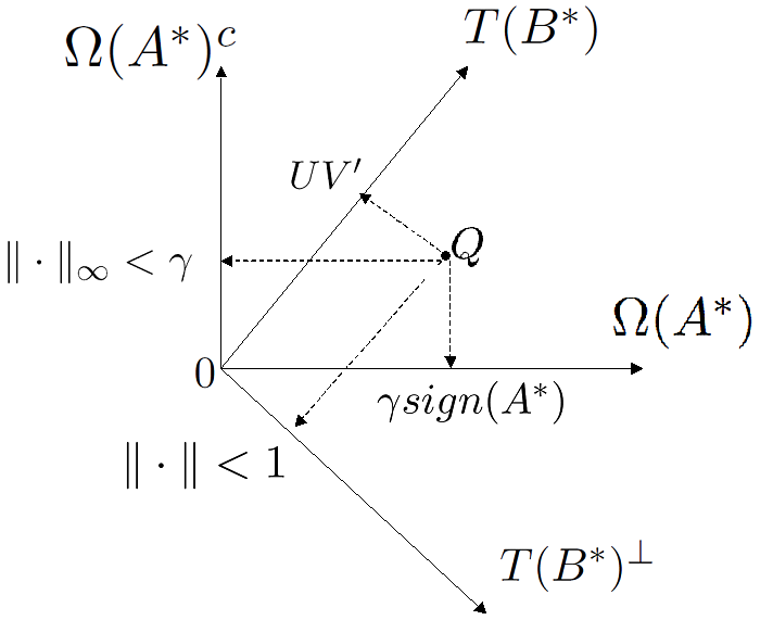
Fig. 1: Geometric representation of optimality conditions: Existence of a dual $Q$. The arrows denote orthogonal projections – every projection must satisfy a condition (according to Proposition 2), which is described next to each arrow.

Proposition 2.

Suppose that $C=A^{\star}+B^{\star}$. Then $(\hat{A},\hat{B})=(A^{\star},B^{\star})$ is the unique optimizer of (3) if the following conditions are satisfied:

1. $\Omega(A^{\star})\cap T(B^{\star})=\{0\}$.

2. There exists a dual $Q\in\mathbb{R}^{n\times n}$ such that

   1. $P_{T(B^{\star})}(Q)=UV^{\prime}$

   2. $P_{\Omega(A^{\star})}(Q)=\gamma\mathrm{sign}(A^{\star})$

   3. $\|P_{T(B^{\star})^{\bot}}(Q)\|<1$

   4. $\|P_{\Omega(A^{\star})^{c}}(Q)\|_{\infty}<\gamma$

The proof of the proposition can be found in Appendix B. Figure 1 provides a visual representation of these conditions. In particular, we see that the spaces $\Omega(A^{\star})$ and $T(B^{\star})$ intersect transversely (part $(1)$ of Proposition 2). One can also intuitively see that guaranteeing the existence of a dual $Q$ with the requisite conditions (part $(2)$ of Proposition 2) is perhaps easier if the intersection between $\Omega(A^{\star})$ and $T(B^{\star})$ is more transverse. Note that condition $(1)$ of this proposition essentially requires identifiability with respect to the tangent spaces, as discussed in Section 3.2.

4.2 Sufficient conditions based on $\mu(A^{\star})$ and $\xi(B^{\star})$

Next we provide simple sufficient conditions on $A^{\star}$ and $B^{\star}$ that guarantee the existence of an appropriate dual $Q$ (as required by Proposition 2). Given matrices $A^{\star}$ and $B^{\star}$ with $\mu(A^{\star})\xi(B^{\star})<1$, we have from Proposition 1 that $\Omega(A^{\star})\cap T(B^{\star})=\{0\}$, i.e., condition $(1)$ of Proposition 2 is satisfied. We prove that if a slightly stronger condition holds, there exists a dual $Q$ that satisfies the requirements of condition $(2)$ of Proposition 2.

Theorem 2.

Given $C=A^{\star}+B^{\star}$ with

$$\mu(A^{\star})\xi(B^{\star})<\frac{1}{6}$$

the unique optimum $(\hat{A},\hat{B})$ of (3) is $(A^{\star},B^{\star})$ for the following range of $\gamma$:

$$\gamma\in\left(\frac{\xi(B^{\star})}{1-4\mu(A^{\star})\xi(B^{\star})},\frac{1-3\mu(A^{\star})\xi(B^{\star})}{\mu(A^{\star})}\right).$$

Specifically $\gamma=\sqrt{\frac{3\xi(B^{\star})}{2\mu(A^{\star})}}$ is always inside the above range, and thus guarantees exact recovery of $(A^{\star},B^{\star})$.

The proof of this theorem can be found in Appendix B. The main idea behind the proof is that we only consider candidates for the dual $Q$ that lie in the direct sum $\Omega(A^{\star})\oplus T(B^{\star})$ of the tangent spaces. Since $\mu(A^{\star})\xi(B^{\star})<\frac{1}{6}$, we have from Proposition 1 that the tangent spaces $\Omega(A^{\star})$ and $T(B^{\star})$ have a transverse intersection, i.e., $\Omega(A^{\star})\cap T(B^{\star})=\{0\}$. Therefore, there exists a unique element $\hat{Q}\in\Omega(A^{\star})\oplus T(B^{\star})$ that satisfies $P_{T(B^{\star})}(\hat{Q})=UV^{\prime}$ and $P_{\Omega(A^{\star})}(\hat{Q})=\gamma\mathrm{sign}(A^{\star})$. The proof proceeds by showing that if $\mu(A^{\star})\xi(B^{\star})<\frac{1}{6}$ then the projections of this $\hat{Q}$ onto the orthogonal spaces $\Omega(A^{\star})^{c}$ and $T(B^{\star})^{\bot}$ are small, thus satisfying condition $(2)$ of Proposition 2.

Remarks

One consequence of Theorem 2 is that if $\mu(A^{\star})\xi(B^{\star})<\frac{1}{6}$, then there exists no other $(A,B)$ such that $A+B=A^{\star}+B^{\star}$ with $\mu(A)\xi(B)<\frac{1}{6}$. We consider this implication locally around $(A^{\star},B^{\star})$. Recall that the quantities $\mu(A^{\star})$ and $\xi(B^{\star})$ are defined with respect to the tangent spaces $\Omega(A^{\star})$ and $T(B^{\star})$. Suppose $B^{\star}$ is slightly perturbed along the variety of rank-constrained matrices to some $B$. This ensures that the tangent space varies smoothly from $T(B^{\star})$ to $T(B)$, and consequently that $\xi(B)\approx\xi(B^{\star})$. However, compensating for this by changing $A^{\star}$ to $A^{\star}+(B^{\star}-B)$ moves $A^{\star}$ outside the variety of sparse matrices. This is because $B^{\star}-B$ is not sparse. Thus the dimension of the tangent space $\Omega(A^{\star}+B^{\star}-B)$ is much greater than that of the tangent space $\Omega(A^{\star})$, as a result of which $\mu(A^{\star}+B^{\star}-B)\gg\mu(A^{\star})$; therefore we have that $\xi(B)\mu(A^{\star}+B^{\star}-B)\gg\frac{1}{6}$. The same reasoning holds in the opposite scenario. Consider perturbing $A^{\star}$ slightly along the variety of sparse matrices to some $A$. While this ensures that $\mu(A)\approx\mu(A^{\star})$, changing $B^{\star}$ to $B^{\star}+(A^{\star}-A)$ moves $B^{\star}$ outside the variety of rank-constrained matrices. Therefore the dimension of the tangent space $T(B^{\star}+A^{\star}-A)$ is greater than that of $T(B^{\star})$, resulting in $\xi(B^{\star}+A^{\star}-A)\gg\xi(B^{\star})$; consequently we have that $\mu(A)\xi(B^{\star}+A^{\star}-A)\gg\frac{1}{6}$.

4.3 Sparse and low-rank matrices with $\mu(A^{\star})\xi(B^{\star})<\frac{1}{6}$

We discuss concrete classes of sparse and low-rank matrices that satisfy the sufficient condition of Theorem 2 for exact decomposition. We begin by showing that sparse matrices with “bounded degree”, i.e., bounded number of non-zeros per row/column, have small $\mu$.

Proposition 3.

Let $A\in\mathbb{R}^{n\times n}$ be any matrix with at most $\mathrm{deg}_{\mathrm{max}}(A)$ non-zero entries per row/column, and with at least $\mathrm{deg}_{\mathrm{min}}(A)$ non-zero entries per row/column. With $\mu(A)$ as defined in (2), we have that

$$\mathrm{deg}_{\mathrm{min}}(A)\leq\mu(A)\leq\mathrm{deg}_{\mathrm{max}}(A).$$

See Appendix B for the proof. Note that if $A\in\mathbb{R}^{n\times n}$ has full support, i.e., $\Omega(A)=\mathbb{R}^{n\times n}$, then $\mu(A)=n$. Therefore, a constraint on the number of zeros per row/column provides a useful bound on $\mu$. We emphasize here that simply bounding the number of non-zero entries in $A$ does not suffice; the sparsity pattern also plays a role in determining the value of $\mu$.

Next we consider low-rank matrices that have small $\xi$. Specifically, we show that matrices with row and column spaces that are incoherent with respect to the standard basis have small $\xi$. We measure the incoherence of a subspace $S\subseteq\mathbb{R}^{n}$ as follows:

$$\beta(S)\triangleq\max_{i}\|P_{S}e_{i}\|_{2},$$ (14)

where $e_{i}$ is the $i$’th standard basis vector, $P_{S}$ denotes the projection onto the subspace $S$, and $\|\cdot\|_{2}$ denotes the vector $\ell_{2}$ norm. This definition of incoherence also played an important role in the results in [4]. A small value of $\beta(S)$ implies that the subspace $S$ is not closely aligned with any of the coordinate axes. In general for any $k$-dimensional subspace $S$, we have that

$$\sqrt{\frac{k}{n}}\leq\beta(S)\leq 1,$$

where the lower bound is achieved, for example, by a subspace that spans any $k$ columns of an $n\times n$ orthonormal Hadamard matrix, while the upper bound is achieved by any subspace that contains a standard basis vector. Based on the definition of $\beta(S)$, we define the incoherence of the row/column spaces of a matrix $B\in\mathbb{R}^{n\times n}$ as

$$\mathrm{inc}(B)\triangleq\max\{\beta(\mathrm{row\mbox{-}space}(B)),~{}\beta(\mathrm{column\mbox{-}space}(B))\}.$$ (15)

If the SVD of $B=U\Sigma V^{T}$ then $\mathrm{row\mbox{-}space}(B)=\mathrm{span}(V)$ and $\mathrm{column\mbox{-}space}(B)=\mathrm{span}(U)$. We show in Appendix B that matrices with incoherent row/column spaces have small $\xi$; the proof technique for the lower bound here was suggested by Ben Recht [23].

Proposition 4.

Let $B\in\mathbb{R}^{n\times n}$ be any matrix with $\mathrm{inc}(B)$ defined as in (15), and $\xi(B)$ defined as in (1). We have that

$$\mathrm{inc}(B)\leq\xi(B)\leq 2~{}\mathrm{inc}(B).$$

If $B\in\mathbb{R}^{n\times n}$ is a full-rank matrix or a matrix such as $e_{1}e_{1}^{T}$, then $\xi(B)=1$. Therefore, a bound on the incoherence of the row/column spaces of $B$ is important in order to bound $\xi$. Using Propositions 3 and 4 along with Theorem 2 we have the following corollary, which states that sparse bounded-degree matrices and low-rank matrices with incoherent row/column spaces can be uniquely decomposed.

Corollary 3.

Let $C=A^{\star}+B^{\star}$ with $\mathrm{deg}_{\mathrm{max}}(A^{\star})$ being the maximum number of nonzero entries per row/column of $A^{\star}$ and $\mathrm{inc}(B^{\star})$ being the maximum incoherence of the row/column spaces of $B^{\star}$ (as defined by (15)). If we have that

$$\mathrm{deg}_{\mathrm{max}}(A^{\star})~{}\mathrm{inc}(B^{\star})<\frac{1}{12},$$

then the unique optimum of the convex program (3) is $(\hat{A},\hat{B})=(A^{\star},B^{\star})$ for a range of values of $\gamma$:

$$\gamma\in\left(\frac{2~{}\mathrm{inc}(B^{\star})}{1-8~{}\mathrm{deg}_{\mathrm{max}}(A^{\star})~{}\mathrm{inc}(B^{\star})},\frac{1-6~{}\mathrm{deg}_{\mathrm{max}}(A^{\star})~{}\mathrm{inc}(B^{\star})}{\mathrm{deg}_{\mathrm{max}}(A^{\star})}\right).$$ (16)

Specifically $\gamma=\sqrt{\frac{3~{}\mathrm{inc}(B^{\star})}{\mathrm{deg}_{\mathrm{max}}(A^{\star})}}$ is always inside the above range, and thus guarantees exact recovery of $(A^{\star},B^{\star})$.

We emphasize that this is a result with deterministic sufficient conditions on exact decomposability.

4.4 Decomposing random sparse and low-rank matrices

Next we show that sparse and low-rank matrices drawn from certain natural random ensembles satisfy the sufficient conditions of Corollary 3 with high probability. We first consider random sparse matrices with a fixed number of non-zero entries.

Random sparsity model

The matrix $A^{\star}$ is such that $\mathrm{support}(A^{\star})$ is chosen uniformly at random from the collection of all support sets of size $m$. There is no assumption made about the values of $A^{\star}$ at locations specified by $\mathrm{support}(A^{\star})$.

Lemma 1.

Suppose that $A^{\star}\in\mathbb{R}^{n\times n}$ is drawn according to the random sparsity model with $m$ non-zero entries. Let $\mathrm{deg}_{\mathrm{max}}(A^{\star})$ be the maximum number of non-zero entries in each row/column of $A^{\star}$. We have that

$$\mathrm{deg}_{\mathrm{max}}(A^{\star})\leq\frac{m}{n}\log(n),$$

with high probability.

The proof of this lemma follows from a standard balls and bins argument, and can be found in several references (see for example [2]).

Next we consider low-rank matrices in which the singular vectors are chosen uniformly at random from the set of all partial isometries. Such a model was considered in recent work on the matrix completion problem [4], which aims to recover a low-rank matrix given observations of a subset of entries of the matrix.

Random orthogonal model [4]

A rank-$k$ matrix $B^{\star}\in\mathbb{R}^{n\times n}$ with SVD $B^{\star}=U\Sigma V^{\prime}$ is constructed as follows: The singular vectors $U,V\in\mathbb{R}^{n\times k}$ are drawn uniformly at random from the collection of rank-$k$ partial isometries in $\mathbb{R}^{n\times k}$. The choices of $U$ and $V$ need not be mutually independent. No restriction is placed on the singular values.

As shown in [4], low-rank matrices drawn from such a model have incoherent row/column spaces.

Lemma 2.

Suppose that a rank-$k$ matrix $B^{\star}\in\mathbb{R}^{n\times n}$ is drawn according to the random orthogonal model. Then we have that that $\mathrm{inc}(B^{\star})$ (defined by (15)) is bounded as

$$\mathrm{inc}(B^{\star})\lesssim\sqrt{\frac{\max(k,\log(n))}{n}},$$

with very high probability.

Applying these two results in conjunction with Corollary 3, we have that sparse and low-rank matrices drawn from the random sparsity model and the random orthogonal model can be uniquely decomposed with high probability.

Corollary 4.

Suppose that a rank-$k$ matrix $B^{\star}\in\mathbb{R}^{n\times n}$ is drawn from the random orthogonal model, and that $A^{\star}\in\mathbb{R}^{n\times n}$ is drawn from the random sparsity model with $m$ non-zero entries. Given $C=A^{\star}+B^{\star}$, there exists a range of values for $\gamma$ (given by (16)) so that $(\hat{A},\hat{B})=(A^{\star},B^{\star})$ is the unique optimum of the SDP (3) with high probability provided

$$m\lesssim\frac{n^{1.5}}{\log n\sqrt{\max(k,\log n)}}.$$

Thus, for matrices $B^{\star}$ with rank $k$ smaller than $n$ the SDP (3) yields exact recovery with high probability even when the size of the support of $A^{\star}$ is super-linear in $n$. During final preparation of this manuscript we learned of related contemporaneous work [30] that specifically studies the problem of decomposing random sparse and low-rank matrices. In addition to the assumptions of our random sparsity and random orthogonal models, [30] also requires that the non-zero entries of $A^{\star}$ have independently chosen signs that are $\pm 1$ with equal probability, while the left and right singular vectors of $B^{\star}$ are chosen independent of each other. For this particular specialization of our more general framework, the results in [30] improve upon our bound in Corollary 4.

Implications for the matrix rigidity problem

Corollary 4 has implications for the matrix rigidity problem discussed in Section 2. Recall that $R_{M}(k)$ is the smallest number of entries of $M$ that need to be changed to reduce the rank of $M$ below $k$ (the changes can be of arbitrary magnitude). A generic matrix $M\in\mathbb{R}^{n\times n}$ has rigidity $R_{M}(k)=(n-k)^{2}$ [27]. However, special structured classes of matrices can have low rigidity. Consider a matrix $M$ formed by adding a sparse matrix drawn from the random sparsity model with support size $\mathcal{O}(\frac{n}{\log n})$, and a low-rank matrix drawn from the random orthogonal model with rank $\epsilon n$ for some fixed $\epsilon>0$. Such a matrix has rigidity $R_{M}(\epsilon n)=\mathcal{O}(\frac{n}{\log n})$, and one can recover the sparse and low-rank components that compose $M$ with high probability by solving the SDP (3). To see this, note that

$$\frac{n}{\log n}\lesssim\frac{n^{1.5}}{\log n\sqrt{\max(\epsilon n,\log n)}}=\frac{n^{1.5}}{\log n\sqrt{\epsilon n}},$$

which satisfies the sufficient condition of Corollary 4 for exact recovery. Therefore, while the rigidity of a matrix is NP-hard to compute in general [7], for such low-rigidity matrices $M$ one can compute the rigidity $R_{M}(\epsilon n)$; in fact the SDP (3) provides a certificate of the sparse and low-rank matrices that form the low rigidity matrix $M$.

5 Simulation Results

We confirm the theoretical predictions in this paper with some simple experimental results. We also present a heuristic to choose the trade-off parameter $\gamma$. All our simulations were performed using YALMIP [31] and the SDPT3 software [26] for solving SDPs.

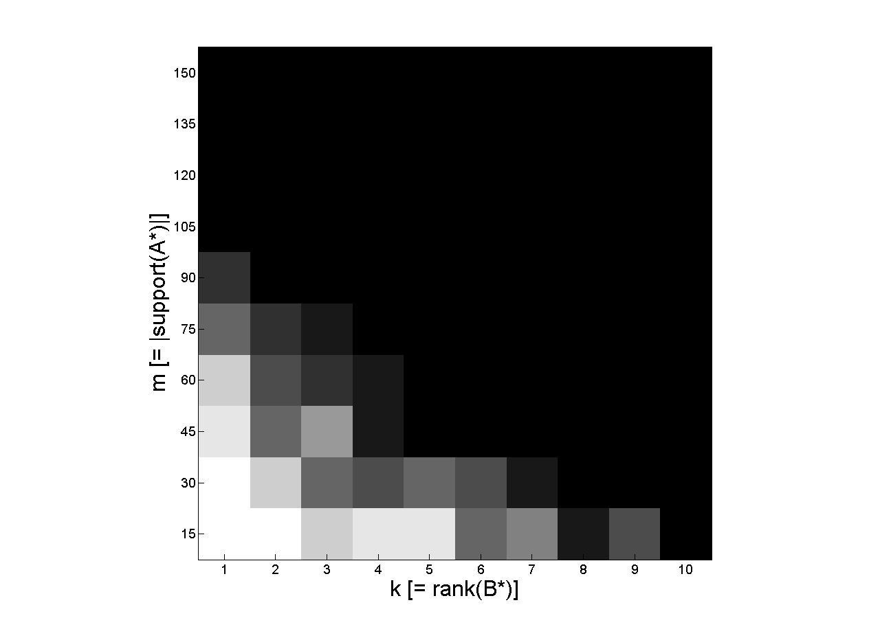
Fig. 2: For each value of $m,k$, we generate $25\times 25$ random $m$-sparse $A^{\star}$ and random rank-$k$ $B^{\star}$ and attempt to recover $(A^{\star},B^{\star})$ from $C=A^{\star}+B^{\star}$ using (3). For each value of $m,k$ we repeated this procedure $10$ times. The figure shows the probability of success in recovering $(A^{\star},B^{\star})$ using (3) for various values of $m$ and $k$. White represents a probability of success of $1$, while black represents a probability of success of $0$.

In the first experiment we generate random $25\times 25$ matrices according to the random sparsity and random orthogonal models described in Section 4.4. To generate a random rank-$k$ matrix $B^{\star}$ according to the random orthogonal model, we generate $X,Y\in\mathbb{R}^{25\times k}$ with i.i.d. Gaussian entries and set $B^{\star}=XY^{T}$. To generate an $m$-sparse matrix $A^{\star}$ according to the random sparsity model, we choose a support set of size $m$ uniformly at random and the values within this support are i.i.d. Gaussian. The goal is to recover $(A^{\star},B^{\star})$ from $C=A^{\star}+B^{\star}$ using the SDP (3). Let $\mathrm{tol}_{\gamma}$ be defined as:

$$\mathrm{tol}_{\gamma}=\frac{\|\hat{A}-A^{\star}\|_{F}}{\|A^{\star}\|_{F}}+\frac{\|\hat{B}-B^{\star}\|_{F}}{\|B^{\star}\|_{F}},$$ (17)

where $(\hat{A},\hat{B})$ is the solution of (3), and $\|\cdot\|_{F}$ is the Frobenius norm. We declare success in recovering $(A^{\star},B^{\star})$ if $\mathrm{tol}_{\gamma}<10^{-3}$. (We discuss the issue of choosing $\gamma$ in the next experiment.) Figure 2 shows the success rate in recovering $(A^{\star},B^{\star})$ for various values of $m$ and $k$ (averaged over $10$ experiments for each $m,k$). Thus we see that one can recover sufficiently sparse $A^{\star}$ and sufficiently low-rank $B^{\star}$ from $C=A^{\star}+B^{\star}$ using (3).

Fig. 3: Comparison between $\mathrm{tol}_{t}$ and $\mathrm{diff}_{t}$ for a randomly generated example with $n=25,m=25,k=2$.

Next we consider the problem of choosing the trade-off parameter $\gamma$. Based on Theorem 2 we know that exact recovery is possible for a range of $\gamma$. Therefore, one can simply check the stability of the solution $(\hat{A},\hat{B})$ as $\gamma$ is varied without knowing the appropriate range for $\gamma$ in advance. To formalize this scheme we consider the following SDP for $t\in[0,1]$, which is a slightly modified version of (3):

$$(\hat{A}_{t},\hat{B}_{t})=\arg\min_{A,B} ~{}~{}t\|A\|_{1}+(1-t)\|B\|_{\ast}$$

s.t. $$~{}~{}A+B=C.$$ (18)

There is a one-to-one correspondence between (3) and (18) given by $t=\frac{\gamma}{1+\gamma}$. The benefit in looking at (18) is that the range of valid parameters is compact, i.e., $t\in[0,1]$, as opposed to the situation in (3) where $\gamma\in[0,\infty)$. We compute the difference between solutions for some $t$ and $t-\epsilon$ as follows:

$$\mathrm{diff}_{t}=(\|\hat{A}_{t-\epsilon}-\hat{A}_{t}\|_{F})+(\|\hat{B}_{t-\epsilon}-\hat{B}_{t}\|_{F}),$$ (19)

where $\epsilon>0$ is some small fixed constant, say $\epsilon=0.01$. We generate a random $A^{\star}\in\mathbb{R}^{25\times 25}$ that is $25$-sparse and a random $B^{\star}\in\mathbb{R}^{25\times 25}$ with rank $=2$ as described above. Given $C=A^{\star}+B^{\star}$, we solve (18) for various values of $t$. Figure 3 shows two curves – one is $\mathrm{tol}_{t}$ (which is defined analogous to $\mathrm{tol}_{\gamma}$ in (17)) and the other is $\mathrm{diff}_{t}$. Clearly we do not have access to $\mathrm{tol}_{t}$ in practice. However, we see that $\mathrm{diff}_{t}$ is near-zero in exactly three regions. For sufficiently small $t$ the optimal solution to (18) is $(\hat{A}_{t},\hat{B}_{t})=(A^{\star}+B^{\star},0)$, while for sufficiently large $t$ the optimal solution is $(\hat{A}_{t},\hat{B}_{t})=(0,A^{\star}+B^{\star})$. As seen in the figure, $\mathrm{diff}_{t}$ stabilizes for small and large $t$. The third “middle” range of stability is where we typically have $(\hat{A}_{t},\hat{B}_{t})=(A^{\star},B^{\star})$. Notice that outside of these three regions $\mathrm{diff}_{t}$ is not close to $0$ and in fact changes rapidly. Therefore if a reasonable guess for $t$ (or $\gamma$) is not available, one could solve (18) for a range of $t$ and choose a solution corresponding to the “middle” range in which $\mathrm{diff}_{t}$ is stable and near zero. A related method to check for stability is to compute the sensitivity of the cost of the optimal solution with respect to $\gamma$, which can be obtained from the dual solution.

6 Discussion

We have studied the problem of exactly decomposing a given matrix $C=A^{\star}+B^{\star}$ into its sparse and low-rank components $A^{\star}$ and $B^{\star}$. This problem arises in a number of applications in model selection, system identification, complexity theory, and optics. We characterized fundamental identifiability in the decomposition problem based on a notion of rank-sparsity incoherence, which relates the sparsity pattern of a matrix and its row/column spaces via an uncertainty principle. As the general decomposition problem is NP-hard we propose a natural SDP relaxation (3) to solve the problem, and provide sufficient conditions on sparse and low-rank matrices so that the SDP exactly recovers such matrices. Our sufficient conditions are deterministic in nature; they essentially require that the sparse matrix must have support that is not too concentrated in any row/column, while the low-rank matrix must have row/column spaces that are not closely aligned with the coordinate axes. Our analysis centers around studying the tangent spaces with respect to the algebraic varieties of sparse and low-rank matrices. Indeed the sufficient conditions for identifiability and for exact recovery using the SDP can also be viewed as requiring that certain tangent spaces have a transverse intersection. We also demonstrated the implications of our results for the matrix rigidity problem.

An interesting problem for further research is the development of special-purpose algorithms that take advantage of structure in (3) to provide a more efficient solution than a general-purpose SDP solver. Another question that arises in applications such as model selection (due to noise or finite sample effects) is to approximately decompose a matrix into sparse and low-rank components.

Appendix A SDP formulation

The problem (3) can be recast as a semidefinite program (SDP). We appeal to the fact that the spectral norm $\|\cdot\|$ is the dual norm of the nuclear norm $\|\cdot\|_{\ast}$:

$$\|M\|_{\ast}=\max\{\mathrm{trace}(M^{\prime}Y)|~{}\|Y\|\leq 1\}.$$

Further, the spectral norm admits a simple semidefinite characterization [22]:

$$\|Y\|=\min_{t}~{}~{}t~{}~{}~{}~{}~{}\mbox{s.t.}\left(\begin{array}[]{cc}tI_{n}&Y\vspace{0.05in}\\ Y^{\prime}&tI_{n}\\ \end{array}\right)\succeq 0.$$

From duality, we can obtain the following SDP characterization of the nuclear norm:

$$\|M\|_{\ast}=\min_{W_{1},W_{2}} ~{}~{}\frac{1}{2}(\mathrm{trace}(W_{1})+\mathrm{trace}(W_{2}))$$

s.t. $$~{}~{}\left(\begin{array}[]{cc}W_{1}&M\vspace{0.05in}\\ M^{\prime}&W_{2}\\ \end{array}\right)\succeq 0.$$

Putting these facts together, (3) can be rewritten as

$$\min_{A,B,W_{1},W_{2},Z} \gamma\mathbf{1}_{n}^{T}Z\mathbf{1}_{n}+\frac{1}{2}(\mathrm{trace}(W_{1}) +\mathrm{trace}(W_{2}))$$ (21)

s.t. $$\left(\begin{array}[]{cc}W_{1}&B\vspace{0.05in}\\ B^{\prime}&W_{2}\\ \end{array}\right) \succeq 0$$

$$-Z_{i,j}\leq A_{i,j} \leq Z_{i,j},\quad\forall(i,j)$$

$$A+B =C.$$

Here, $\mathbf{1}_{n}\in\mathbb{R}^{n}$ refers to the vector that has $1$ in every entry.

Appendix B Proofs

Proof of Proposition 1

We begin by establishing that

$$\max_{N\in T(B^{\star}),~{}\|N\|\leq 1}\|P_{\Omega(A^{\star})}(N)\|<1\quad\Rightarrow\quad\Omega(A^{\star})~{}\cap~{}T(B^{\star})=\{0\},$$ (22)

where $P_{\Omega(A^{\star})}(N)$ denotes the projection onto the space $\Omega(A^{\star})$. Assume for the sake of a contradiction that this assertion is not true. Thus, there exists $N\neq 0$ such that $N\in\Omega(A^{\star})\cap T(B^{\star})$. Scale $N$ appropriately such that $\|N\|=1$. Thus $N\in T(B^{\star})$ with $\|N\|=1$, but we also have that $\|P_{\Omega(A^{\star})}(N)\|=\|N\|=1$ as $N\in\Omega(A^{\star})$. This leads to a contradiction.

Next, we show that

$$\max_{N\in T(B^{\star}),~{}\|N\|\leq 1}\|P_{\Omega(A^{\star})}(N)\|\leq\mu(A^{\star})\xi(B^{\star}),$$

which would allow us to conclude the proof of this proposition. We have the following sequence of inequalities

$$\max_{N\in T(B^{\star}),~{}\|N\|\leq 1}\|P_{\Omega(A^{\star})}(N)\| \leq \max_{N\in T(B^{\star}),~{}\|N\|\leq 1}\mu(A^{\star})\|P_{\Omega(A^{\star})}(N)\|_{\infty}$$

$$\leq \max_{N\in T(B^{\star}),~{}\|N\|\leq 1}\mu(A^{\star})\|N\|_{\infty}$$

$$\leq \mu(A^{\star})\xi(B^{\star}).$$

Here the first inequality follows from the definition (2) of $\mu(A^{\star})$ as $P_{\Omega(A^{\star})}(N)\in\Omega(A^{\star})$, the second inequality is due to the fact that $\|P_{\Omega(A^{\star})}(N)\|_{\infty}\leq\|N\|_{\infty}$, and the final inequality follows from the definition (1) of $\xi(B^{\star})$. $\square$

Proof of Proposition 2

We first show that $(A^{\star},B^{\star})$ is an optimum of (3), before moving on to showing uniqueness. Based on subgradient optimality conditions applied at $(A^{\star},B^{\star})$, there must exist a dual $Q$ such that

$$Q\in\gamma\partial\|A^{\star}\|_{1}\quad\mathrm{and}\quad Q\in\partial\|B^{\star}\|_{\ast}.$$

The second condition in this proposition guarantees the existence of a dual $Q$ that satisfies both these subgradient conditions simultaneously (see (12) and (13)). Therefore, we have that $(A^{\star},B^{\star})$ is an optimum. Next we show that under the conditions specified in the lemma, $(A^{\star},B^{\star})$ is also a unique optimum. To avoid cluttered notation, in the rest of this proof we let $\Omega=\Omega(A^{\star})$, $T=T(B^{\star})$, $\Omega^{c}(A^{\star})=\Omega^{c}$, and $T^{\bot}(B^{\star})=T^{\bot}$.

Suppose that there is another feasible solution $(A^{\star}+N_{A},B^{\star}+N_{B})$ that is also a minimizer. We must have that $N_{A}+N_{B}=0$ because $A^{\star}+B^{\star}=C=(A^{\star}+N_{A})+(B^{\star}+N_{B})$. Applying the subgradient property at $(A^{\star},B^{\star})$, we have that for any subgradient $(Q_{A},Q_{B})$ of the function $\gamma\|A\|_{1}+\|B\|_{\ast}$ (at $(A^{\star},B^{\star})$)

$$\gamma\|A^{\star}+N_{A}\|_{1}+\|B^{\star}+N_{B}\|_{\ast}\geq\gamma\|A^{\star}\|_{1}+\|B^{\star}\|_{\ast}+\langle Q_{A},N_{A}\rangle+\langle Q_{B},N_{B}\rangle.$$ (23)

Since $(Q_{A},Q_{B})$ is a subgradient of the function $\gamma\|A\|_{1}+\|B\|_{\ast}$ at $(A^{\star},B^{\star})$, we must have from (12) and (13) that

• $Q_{A}=\gamma\mathrm{sign}(A^{\star})+P_{\Omega^{c}}(Q_{A})$, with $\|P_{\Omega^{c}}(Q_{A})\|_{\infty}\leq\gamma$.

• $Q_{B}=UV^{\prime}+P_{T^{\bot}}(Q_{B})$, with $\|P_{T^{\bot}}(Q_{B})\|\leq 1$.

Using these conditions we rewrite $\langle Q_{A},N_{A}\rangle$ and $\langle Q_{B},N_{B}\rangle$. Based on the existence of the dual $Q$ as described in the lemma, we have that

$$\langle Q_{A},N_{A}\rangle = \langle\gamma\mathrm{sign}(A^{\star})+P_{\Omega^{c}}(Q_{A}),N_{A}\rangle$$ (24)

$$= \langle Q-P_{\Omega^{c}}(Q)+P_{\Omega^{c}}(Q_{A}),N_{A}\rangle$$

$$= \langle P_{\Omega^{c}}(Q_{A})-P_{\Omega^{c}}(Q),N_{A}\rangle+\langle Q,N_{A}\rangle,$$

where we have used the fact that $Q=\gamma\mathrm{sign}(A^{\star})+P_{\Omega^{c}}(Q)$. Similarly, we have that

$$\langle Q_{B},N_{B}\rangle = \langle UV^{\prime}+P_{T^{\bot}}(Q_{B}),N_{B}\rangle$$ (25)

$$= \langle Q-P_{T^{\bot}}(Q)+P_{T^{\bot}}(Q_{B}),N_{B}\rangle$$

$$= \langle P_{T^{\bot}}(Q_{B})-P_{T^{\bot}}(Q),N_{B}\rangle+\langle Q,N_{B}\rangle,$$

where we have used the fact that $Q=UV^{\prime}+P_{T^{\bot}}(Q)$. Putting (24) and (25) together, we have that

$$\langle Q_{A},N_{A}\rangle+\langle Q_{B},N_{B}\rangle = \langle P_{\Omega^{c}}(Q_{A})-P_{\Omega^{c}}(Q),N_{A}\rangle$$ (26)

$$+\langle P_{T^{\bot}}(Q_{B})-P_{T^{\bot}}(Q),N_{B}\rangle$$

$$+\langle Q,N_{A}+N_{B}\rangle$$

$$= \langle P_{\Omega^{c}}(Q_{A})-P_{\Omega^{c}}(Q),N_{A}\rangle$$

$$+\langle P_{T^{\bot}}(Q_{B})-P_{T^{\bot}}(Q),N_{B}\rangle$$

$$= \langle P_{\Omega^{c}}(Q_{A})-P_{\Omega^{c}}(Q),P_{\Omega^{c}}(N_{A})\rangle$$

$$+\langle P_{T^{\bot}}(Q_{B})-P_{T^{\bot}}(Q),P_{T^{\bot}}(N_{B})\rangle.$$

In the second equality, we used the fact that $N_{A}+N_{B}=0$.

Since $(Q_{A},Q_{B})$ is any subgradient, we have some freedom in selecting $P_{\Omega^{c}}(Q_{A})$ and $P_{T^{\bot}}(Q_{B})$ as long as they still satisfy the subgradient conditions $\|P_{\Omega^{c}}(Q_{A})\|_{\infty}\leq\gamma$ and $\|P_{T^{\bot}}(Q_{B})\|\leq 1$. We set $P_{\Omega^{c}}(Q_{A})=\gamma\mathrm{sign}(P_{\Omega^{c}}(N_{A}))$ so that $\|P_{\Omega^{c}}(Q_{A})\|_{\infty}=\gamma$ and $\langle P_{\Omega^{c}}(Q_{A}),P_{\Omega^{c}}(N_{A})\rangle=\gamma\|P_{\Omega^{c}}(N_{A})\|_{1}$. Letting $P_{T^{\bot}}(N_{B})=\tilde{U}\tilde{\Sigma}\tilde{V}^{T}$ be the singular value decomposition of $P_{T^{\bot}}(N_{B})$, we set $P_{T^{\bot}}(Q_{B})=\tilde{U}\tilde{V}^{T}$ so that $\|P_{T^{\bot}}(Q_{B})\|=1$ and $\langle P_{T^{\bot}}(Q_{B}),P_{T^{\bot}}(N_{B})\rangle=\|P_{T^{\bot}}(N_{B})\|_{\ast}$. Consequently, we can simplify (26) as follows:

$$\langle Q_{A},N_{A}\rangle+\langle Q_{B},N_{B}\rangle \geq (\gamma-\|P_{\Omega^{c}}(Q)\|_{\infty})(\|P_{\Omega^{c}}(N_{A})\|_{1})$$

$$+(1-\|P_{T^{\bot}}(Q)\|)(\|P_{T^{\bot}}(N_{B})\|_{\ast}).$$

Since $\|P_{\Omega^{c}}(Q)\|_{\infty}<\gamma$ and $\|P_{T^{\bot}}(Q)\|<1$, we have that $\langle Q_{A},N_{A}\rangle+\langle Q_{B},N_{B}\rangle$ is strictly positive unless $P_{\Omega^{c}}(N_{A})=0$ and $P_{T^{\bot}}(N_{B})=0$. (Note that if $\langle Q_{A},N_{A}\rangle+\langle Q_{B},N_{B}\rangle>0$ then $\gamma\|A^{\star}+N_{A}\|_{1}+\|B^{\star}+N_{B}\|_{\ast}>\gamma\|A^{\star}\|_{1}+\|B^{\star}\|_{\ast}$.) However, we have that $N_{A}+N_{B}=0$. If $P_{\Omega^{c}}(N_{A})=P_{T^{\bot}}(N_{B})=0$, then $P_{\Omega}(N_{A})+P_{T}(N_{B})=0$. In other words, $P_{\Omega}(N_{A})=-P_{T}(N_{B})$. This can only be possible if $P_{\Omega}(N_{A})=P_{T}(N_{B})=0$ (as $\Omega\cap T=\{0\}$), which implies that $N_{A}=N_{B}=0$. Therefore, $\gamma\|A^{\star}+N_{A}\|_{1}+\|B^{\star}+N_{B}\|_{\ast}>\gamma\|A^{\star}\|_{1}+\|B^{\star}\|_{\ast}$ unless $N_{A}=N_{B}=0$. $\square$

Proof of Theorem 2

As with the previous proof, we avoid cluttered notation by letting $\Omega=\Omega(A^{\star})$, $T=T(B^{\star})$, $\Omega^{c}(A^{\star})=\Omega^{c}$, and $T^{\bot}(B^{\star})=T^{\bot}$. One can check that

$$\xi(B^{\star})\mu(A^{\star})<\frac{1}{6}\Rightarrow\frac{\xi(B^{\star})}{1-4\xi(B^{\star})\mu(A^{\star})}<\frac{1-3\xi(B^{\star})\mu(A^{\star})}{\mu(A^{\star})}.$$ (27)

Thus, we show that if $\xi(B^{\star})\mu(A^{\star})<\frac{1}{6}$ then there exists a range of $\gamma$ for which a dual $Q$ with the requisite properties exists. Also note that plugging in $\xi(B^{\star})\mu(A^{\star})=\tfrac{1}{6}$ in the above range gives the smaller range $(3\xi(B^{\star}),\frac{1}{2\mu(A^{\star})})$ for $\gamma$; the geometric mean of the extreme values gives $\gamma=\sqrt{\tfrac{3\xi(B^{\star})}{2\mu(A^{\star})}}$, which is always within the above range.

We aim to construct a dual $Q$ by considering candidates in the direct sum $\Omega\oplus T$ of the tangent spaces. Since $\mu(A^{\star})\xi(B^{\star})<\frac{1}{6}$, we can conclude from Proposition 1 that there exists a unique $\hat{Q}\in\Omega\oplus T$ such that $P_{\Omega}(\hat{Q})=\gamma\mathrm{sign}(A^{\star})$ and $P_{T}(\hat{Q})=UV^{\prime}$ (recall that these are conditions that a dual must satisfy according to Proposition 2), as $\Omega\cap T=\{0\}$. The rest of this proof shows that if $\mu(A^{\star})\xi(B^{\star})<\frac{1}{6}$ then the projections of such a $\hat{Q}$ onto $T^{\bot}$ and onto $\Omega^{c}$ will be small, i.e., we show that $\|P_{\Omega^{c}}(\hat{Q})\|_{\infty}<\gamma$ and $\|P_{T^{\bot}}(\hat{Q})\|<1$.

We note here that $\hat{Q}$ can be uniquely expressed as the sum of an element of $T$ and an element of $\Omega$, i.e., $\hat{Q}=Q_{\Omega}+Q_{T}$ with $Q_{\Omega}\in\Omega$ and $Q_{T}\in T$. The uniqueness of the splitting can be concluded because $\Omega\cap T=\{0\}$. Let $Q_{\Omega}=\gamma\mathrm{sign}(A^{\star})+\epsilon_{\Omega}$ and $Q_{T}=UV^{\prime}+\epsilon_{T}$. We then have

$$P_{\Omega}(\hat{Q})=\gamma\mathrm{sign}(A^{\star})+\epsilon_{\Omega}+P_{\Omega}(Q_{T})=\gamma\mathrm{sign}(A^{\star})+\epsilon_{\Omega}+P_{\Omega}(UV^{\prime}+\epsilon_{T}).$$

Since $P_{\Omega}(\hat{Q})=\gamma\mathrm{sign}(A^{\star})$,

$$\epsilon_{\Omega}=-P_{\Omega}(UV^{\prime}+\epsilon_{T}).$$ (28)

Similarly,

$$\epsilon_{T}=-P_{T}(\gamma\mathrm{sign}(A^{\star})+\epsilon_{\Omega}).$$ (29)

Next, we obtain the following bound on $\|P_{\Omega^{c}}(\hat{Q})\|_{\infty}$:

$$\|P_{\Omega^{c}}(\hat{Q})\|_{\infty} = \|P_{\Omega^{c}}(UV^{\prime}+\epsilon_{T})\|_{\infty}$$ (30)

$$\leq \|UV^{\prime}+\epsilon_{T}\|_{\infty}$$

$$\leq \xi(B^{\star})\|UV^{\prime}+\epsilon_{T}\|$$

$$\leq \xi(B^{\star})(1+\|\epsilon_{T}\|),$$

where we obtain the second inequality based on the definition of $\xi(B^{\star})$ (since $UV^{\prime}+\epsilon_{T}\in T$). Similarly, we can obtain the following bound on $\|P_{T^{\bot}}(\hat{Q})\|$

$$\|P_{T^{\bot}}(\hat{Q})\| = \|P_{T^{\bot}}(\gamma\mathrm{sign}(A^{\star})+\epsilon_{\Omega})\|$$ (31)

$$\leq \|\gamma\mathrm{sign}(A^{\star})+\epsilon_{\Omega}\|$$

$$\leq \mu(A^{\star})\|\gamma\mathrm{sign}(A^{\star})+\epsilon_{\Omega}\|_{\infty}$$

$$\leq \mu(A^{\star})(\gamma+\|\epsilon_{\Omega}\|_{\infty}),$$

where we obtain the second inequality based on the definition of $\mu(A^{\star})$ (since $\gamma\mathrm{sign}(A^{\star})+\epsilon_{\Omega}\in\Omega$). Thus, we can bound $\|P_{\Omega^{c}}(\hat{Q})\|_{\infty}$ and $\|P_{T^{\bot}}(\hat{Q})\|$ by bounding $\|\epsilon_{T}\|$ and $\|\epsilon_{\Omega}\|_{\infty}$ respectively (using the relations (29) and (28)).

By definition of $\xi(B^{\star})$ and using (28),

$$\|\epsilon_{\Omega}\|_{\infty} = \|P_{\Omega}(UV^{\prime}+\epsilon_{T})\|_{\infty}$$ (32)

$$\leq \|UV^{\prime}+\epsilon_{T}\|_{\infty}$$

$$\leq \xi(B^{\star})\|UV^{\prime}+\epsilon_{T}\|$$

$$\leq \xi(B^{\star})(1+\|\epsilon_{T}\|),$$

where the second inequality is obtained because $UV^{\prime}+\epsilon_{T}\in T$. Similarly, by definition of $\mu(A^{\star})$ and using (29)

$$\|\epsilon_{T}\| = \|P_{T}(\gamma\mathrm{sign}(A^{\star})+\epsilon_{\Omega})\|$$ (33)

$$\leq 2\|\gamma\mathrm{sign}(A^{\star})+\epsilon_{\Omega}\|$$

$$\leq 2\mu(A^{\star})\|\gamma\mathrm{sign}(A^{\star})+\epsilon_{\Omega}\|_{\infty}$$

$$\leq 2\mu(A^{\star})(\gamma+\|\epsilon_{\Omega}\|_{\infty}),$$

where the first inequality is obtained because $\|P_{T}(M)\|\leq 2\|M\|$, and the second inequality is obtained because $\gamma\mathrm{sign}(A^{\star})+\epsilon_{\Omega}\in\Omega$.

Putting (32) in (33), we have that

$$\|\epsilon_{T}\| \leq 2\mu(A^{\star})(\gamma+\xi(B^{\star})(1+\|\epsilon_{T}\|))$$

$$\Rightarrow\|\epsilon_{T}\| \leq \frac{2\gamma\mu(A^{\star})+2\xi(B^{\star})\mu(A^{\star})}{1-2\xi(B^{\star})\mu(A^{\star})}.$$ (34)

Similarly, putting (33) in (32), we have that

$$\|\epsilon_{\Omega}\|_{\infty} \leq \xi(B^{\star})(1+2\mu(A^{\star})(\gamma+\|\epsilon_{\Omega}\|_{\infty}))$$

$$\Rightarrow\|\epsilon_{\Omega}\|_{\infty} \leq \frac{\xi(B^{\star})+2\gamma\xi(B^{\star})\mu(A^{\star})}{1-2\xi(B^{\star})\mu(A^{\star})}.$$ (35)

We now show that $\|P_{T^{\bot}}(\hat{Q})\|<1$. Combining (35) and (31),

$$\|P_{T^{\bot}}(\hat{Q})\| \leq \mu(A^{\star})\left(\gamma+\frac{\xi(B^{\star})+2\gamma\xi(B^{\star})\mu(A^{\star})}{1-2\xi(B^{\star})\mu(A^{\star})}\right)$$

$$= \mu(A^{\star})\left(\frac{\gamma+\xi(B^{\star})}{1-2\xi(B^{\star})\mu(A^{\star})}\right)$$

$$< \mu(A^{\star})\left(\frac{\frac{1-3\xi(B^{\star})\mu(A^{\star})}{\mu(A^{\star})}+\xi(B^{\star})}{1-2\xi(B^{\star})\mu(A^{\star})}\right)$$

$$= 1,$$

since $\gamma<\frac{1-3\xi(B^{\star})\mu(A^{\star})}{\mu(A^{\star})}$ by assumption.

Finally, we show that $\|P_{\Omega^{c}}(\hat{Q})\|_{\infty}<\gamma$. Combining (34) and (30),

$$\|P_{\Omega^{c}}(\hat{Q})\|_{\infty} \leq \xi(B^{\star})\left(1+\frac{2\gamma\mu(A^{\star})+2\xi(B^{\star})\mu(A^{\star})}{1-2\xi(B^{\star})\mu(A^{\star})}\right)$$

$$= \xi(B^{\star})\left(\frac{1+2\gamma\mu(A^{\star})}{1-2\xi(B^{\star})\mu(A^{\star})}\right)$$

$$= \left[\xi(B^{\star})\left(\frac{1+2\gamma\mu(A^{\star})}{1-2\xi(B^{\star})\mu(A^{\star})}\right)-\gamma\right]+\gamma$$

$$= \left[\frac{\xi(B^{\star})+2\gamma\xi(B^{\star})\mu(A^{\star})-\gamma+2\gamma\xi(B^{\star})\mu(A^{\star})}{1-2\xi(B^{\star})\mu(A^{\star})}\right]+\gamma$$

$$= \left[\frac{\xi(B^{\star})-\gamma(1-4\xi(B^{\star})\mu(A^{\star}))}{1-2\xi(B^{\star})\mu(A^{\star})}\right]+\gamma$$

$$< \left[\frac{\xi(B^{\star})-\xi(B^{\star})}{1-2\xi(B^{\star})\mu(A^{\star})}\right]+\gamma$$

$$= \gamma.$$

Here, we used the fact that $\frac{\xi(B^{\star})}{1-4\xi(B^{\star})\mu(A^{\star})}<\gamma$ in the second inequality. $\square$

Proof of Proposition 3

Based on the Perron-Frobenius theorem [17], one can conclude that $\|P\|\geq\|Q\|$ if $P_{i,j}\geq|Q_{i,j}|,~{}\forall~{}i,j$. Thus, we need only consider the matrix that has $1$ in every location in the support set $\Omega(A)$ and $0$ everywhere else. Based on the definition of the spectral norm, we can re-write $\mu(A)$ as follows:

$$\mu(A)=\max_{\|x\|_{2}=1,\|y\|_{2}=1}\sum_{(i,j)\in\Omega(A)}x_{i}y_{j}.$$ (36)

Without loss of generality we restrict our attention to optima that are achieved by element-wise non-negative vectors $x,y$.

Upper bound

Since the reformulation of $\mu(A)$ above involves the maximization of a continuous function over a compact set, the maximum is achieved at some point in the constraint set. Therefore, we have that any optimal $(\hat{x},\hat{y})$ must satisfy the following necessary optimality conditions: There exist Lagrange multipliers $\lambda_{1},\lambda_{2}$ such that

$$\nabla_{x}\left[\sum_{(i,j)\in\Omega(A)}x_{i}y_{j}\right]_{(\hat{x},\hat{y})} = 2\lambda_{1}\hat{x}$$

$$\nabla_{y}\left[\sum_{(i,j)\in\Omega(A)}x_{i}y_{j}\right]_{(\hat{x},\hat{y})} = 2\lambda_{2}\hat{y}$$

This reduces to the following system of equations:

$$\sum_{(i,j)\in\Omega(A)}\hat{y}_{j} = 2\lambda_{1}\hat{x}_{i},~{}~{}\forall i$$ (37)

$$\sum_{(i,j)\in\Omega(A)}\hat{x}_{i} = 2\lambda_{2}\hat{y}_{j},~{}~{}\forall j.$$ (38)

Multiplying the first system of equations (37) element-wise by $\hat{x}$ and then summing, we have that

$$\sum_{i}\hat{x}_{i}\sum_{j:(i,j)\in\Omega(A)}\hat{y}_{j} = \sum_{i}\hat{x}_{i}\times 2\lambda_{1}\hat{x}_{i}$$

$$\Rightarrow\sum_{(i,j)\in\Omega(A)}\hat{x}_{i}\hat{y}_{j} = 2\lambda_{1}.$$

Similarly, we have that $\sum_{(i,j)\in\Omega(A)}\hat{x}_{i}\hat{y}_{j}=2\lambda_{2}$, which implies that the Lagrange multipliers are equal to each other and to one-half of the optimal value attained

$$2\lambda_{1}=2\lambda_{2}=\sum_{(i,j)\in\Omega(A)}\hat{x}_{i}\hat{y}_{j}\triangleq 2\lambda.$$

We recall here that the optimal points $\hat{x},\hat{y}$ are element-wise non-negative. Let $\sigma$ denote the element-wise sum of the optimal points $\hat{x},\hat{y}$:

$$\sigma=\sum_{i}\hat{x}_{i}+\sum_{j}\hat{y}_{j}.$$

Summing over all $i$ in (37) and all $j$ in (38), we have that

$$\sum_{i}\sum_{j:(i,j)\in\Omega(A)}\hat{y}_{j}+\sum_{j}\sum_{i:(i,j)\in\Omega(A)}\hat{x}_{i} = 2\lambda\times\sigma$$

$$\Rightarrow\sum_{(i,j)\in\Omega(A)}\hat{y}_{j}+\sum_{(i,j)\in\Omega(A)}\hat{x}_{i} = 2\lambda\times\sigma$$

$$\Rightarrow\sum_{j}\mathrm{deg}_{\mathrm{max}}(A)\hat{y}_{j}+\sum_{i}\mathrm{deg}_{\mathrm{max}}(A)\hat{x}_{i} \geq 2\lambda\times\sigma$$

$$\Rightarrow\mathrm{deg}_{\mathrm{max}}(A)\times\sigma \geq 2\lambda\times\sigma$$

$$\Rightarrow\mathrm{deg}_{\mathrm{max}}(A) \geq 2\lambda=\sum_{(i,j)\in\Omega(A)}\hat{x}_{i}\hat{y}_{j}.$$

Note that we used the fact that $\sigma\neq 0$. Thus, we have that $\mu(A)\leq\mathrm{deg}_{\mathrm{max}}(A)$.

Lower bound

Now suppose that each row/column of $A$ has at least $\mathrm{deg}_{\mathrm{min}}(A)$ non-zero entries. Using the reformulation (36) of $\mu(A)$ above, we have that

$$\mu(A)\geq\sum_{(i,j)\in\Omega(A)}\frac{1}{\sqrt{n}}\frac{1}{\sqrt{n}}=\frac{|\mathrm{support}(A)|}{n}\geq\mathrm{deg}_{\mathrm{min}}(A).$$

Here we set $x=y=\frac{1}{\sqrt{n}}\mathbf{1},$ with $\mathbf{1}$ representing the all-ones vector, as candidates in the optimization problem (36). $\square$

Proof of Proposition 4

Let $B=U\Sigma V^{T}$ be the SVD of $B$.

Upper bound

We can upper-bound $\xi(B)$ as follows

$$\xi(B) = \max_{M\in T(B),\|M\|\leq 1}\|M\|_{\infty}$$

$$= \max_{M\in T(B),\|M\|\leq 1}\|P_{T(B)}(M)\|_{\infty}$$

$$\leq \max_{\|M\|\leq 1}\|P_{T(B)}(M)\|_{\infty}$$

$$\leq \max_{M\mathrm{~{}unitary}}\|P_{T(B)}(M)\|_{\infty}$$

$$\leq \max_{M\mathrm{~{}unitary}}\|P_{U}M\|_{\infty}+\max_{M\mathrm{~{}unitary}}\|(I_{n\times n}-P_{U})MP_{V}\|_{\infty}.$$

For the second inequality, we have used the fact that the maximum of a convex function over a convex set is achieved at one of the extreme points of the constraint set. The unitary matrices are the extreme points of the set of contractions (i.e., matrices with spectral norm $\leq 1$). We have used $P_{T(B)}(M)=P_{U}M+MP_{V}-P_{U}MP_{V}$ from (9) in the last inequality, where $P_{U}=UU^{T}$ and $P_{V}=VV^{T}$ denote the projections onto the spaces spanned by $U$ and $V$ respectively.

We have the following simple bound for $\|P_{U}M\|_{\infty}$ with $M$ unitary:

$$\max_{M\mathrm{~{}unitary}}\|P_{U}M\|_{\infty} = \max_{M\mathrm{~{}unitary}}\max_{i,j}e_{i}^{T}P_{U}Me_{j}$$ (39)

$$\leq \max_{M\mathrm{~{}unitary}}\max_{i,j}\|P_{U}e_{i}\|_{2}~{}\|Me_{j}\|_{2}$$

$$= \max_{i}\|P_{U}e_{i}\|_{2}~{}\times~{}\max_{M\mathrm{~{}unitary}}\max_{j}\|Me_{j}\|_{2}$$

$$= \beta(U).$$

Here we used the Cauchy-Schwartz inequality in the second line, and the definition of $\beta$ from (14) in the last line.

Similarly, we have that

$$\max_{M\mathrm{~{}unitary}}\|(I_{n\times n}-P_{U})MP_{V}\|_{\infty} = \max_{M\mathrm{~{}unitary}}\max_{i,j}e_{i}^{T}(I_{n\times n}-P_{U})MP_{V}e_{j}$$ (40)

$$\leq \max_{M\mathrm{~{}unitary}}\max_{i,j}\|(I_{n\times n}-P_{U})e_{i}\|_{2}~{}\|MP_{V}e_{j}\|_{2}$$

$$= \max_{i}\|(I_{n\times n}-P_{U})e_{i}\|_{2}~{}\times~{}\max_{M\mathrm{~{}unitary}}\max_{j}\|MP_{V}e_{j}\|_{2}$$

$$\leq 1\times\max_{j}\|P_{V}e_{j}\|_{2}$$

$$= \beta(V).$$

Using the definition of $\mathrm{inc}(B)$ from (15) along with (39) and (40), we have that

$$\xi(B)\leq\beta(U)+\beta(V)\leq 2~{}\mathrm{inc}(B).$$

Lower bound

Next we prove a lower bound on $\xi(B)$. Recall the definition of the tangent space $T(B)$ from (6). We restrict our attention to elements of the tangent space $T(B)$ of the form $P_{U}M=UU^{T}M$ for $M$ unitary (an analogous argument follows for elements of the form $P_{V}M$ for $M$ unitary). One can check that

$$\|P_{U}M\|=\max_{\|x\|_{2}=1,\|y\|_{2}=1}x^{T}P_{U}My\leq\max_{\|x\|_{2}=1}\|P_{U}x\|_{2}~{}\max_{\|y\|_{2}=1}\|My\|_{2}\leq 1.$$

Therefore,

$$\xi(B)\geq\max_{M\mathrm{~{}unitary}}\|P_{U}M\|_{\infty}.$$

Thus, we only need to show that the inequality in line $(2)$ of (39) is achieved by some unitary matrix $M$ in order to conclude that $\xi(B)\geq\beta(U)$. Define the “most aligned” basis vector with the subspace $U$ as follows:

$$i^{\ast}=\arg\max_{i}\|P_{U}e_{i}\|_{2}.$$

Let $M$ be any unitary matrix with one of its columns equal to $\frac{1}{\beta(U)}P_{U}e_{i^{\ast}}$, i.e., a normalized version of the projection onto $U$ of the most aligned basis vector. One can check that such a unitary matrix achieves equality in line $(2)$ of (39). Consequently, we have that

$$\xi(B)\geq\max_{M\mathrm{~{}unitary}}\|P_{U}M\|_{\infty}=\beta(U).$$

By a similar argument with respect to $V$, we have the lower bound as claimed in the proposition. $\square$

References

• [1] D. P. Bertsekas, A. Nedic, and A. E. Ozdaglar, Convex Analysis and Optimization, Athena Scientic, Belmont, MA, 2003.
• [2] B. Bollobás, Random graphs, Cambridge University Press, 2001.
• [3] E. J. Candès, J. Romberg, and T. Tao, Robust uncertainty principles: exact signal reconstruction from highly incomplete frequency information, IEEE Transactions on Information Theory, volume 52, number 2, pages 489–509, 2006.
• [4] E. J. Candès and B. Recht, Exact Matrix Completion Via Convex Optimization, Submitted for publication, 2008.
• [5] V. Chandrasekaran, S. Sanghavi, P. A. Parrilo, and A. S. Willsky, Sparse and Low-rank Matrix Decompositions, Proceedings of the 15th IFAC Symposium on System Identification, 2009.
• [6] V. Chandrasekaran, S. Sanghavi, P. A. Parrilo, and A. S. Willsky, Latent-Variable Gaussian Graphical Model Selection, In preparation.
• [7] B. Codenotti, Matrix rigidity, Linear Algebra and its Applications, volume 304, number 1–3, pages 181–192, 2000.
• [8] D. L. Donoho and X. Huo, Uncertainty principles and ideal atomic decomposition, IEEE Transactions on Information Theory, volume 47, number 7, pages 2845–2862, 2001.
• [9] D. L. Donoho and M. Elad, Optimal Sparse Representation in General (Nonorthogonal) Dictionaries via $\ell_{1}$ Minimization, Proceedings of the National Academy of Sciences, volume 100, pages 2197–2202, 2003.
• [10] D. L. Donoho, For most large underdetermined systems of linear equations the minimal $\ell_{1}$-norm solution is also the sparsest solution, Communications on Pure and Applied Mathematics, volume 59, issue 6, pages 797–829, 2006.
• [11] D. L. Donoho, Compressed sensing, IEEE Transactions on Information Theory, volume 52, number 4, pages 1289–1306, 2006.
• [12] M. Fazel and J. Goodman, Approximations for Partially Coherent Optical Imaging Systems, Technical Report, Department of Electrical Engineering, Stanford University, 1998.
• [13] M. Fazel, Matrix Rank Minimization with Applications, PhD thesis, Department of Electrical Engineering, Stanford University, 2002.
• [14] M. Fazel, H. Hindi, and S. Boyd, Log-det heuristic for matrix rank minimization with applications to Hankel and Euclidean distance matrices, Proceedings of the American Control Conference, 2003.
• [15] J. Goodman, Introduction to Fourier Optics, Roberts and Company Publishers, 2004.
• [16] J. Harris, Algebraic Geometry: A First Course, Springer-Verlag, 1995.
• [17] R. A. Horn and C. R. Johnson, Matrix Analysis, Cambridge University Press, 1990.
• [18] S. L. Lauritzen, Graphical Models, Oxford University Press, 1996.
• [19] S. Lokam, Spectral Methods for Matrix Rigidity with Applications to Size-Depth Tradeoffs and Communication Complexity, 36th IEEE Symposium on Foundations of Computer Science (FOCS), pages 6–15, 1995.
• [20] M. Mesbahi and G. P. Papavassilopoulos, On the rank minimization problem over a positive semidefinite linear matrix inequality, IEEE Transactions on Automatic Control, volume 42, number 2, pages 239 -243, 1997.
• [21] Y. C. Pati and T. Kailath, Phase-shifting masks for microlithography: Automated design and mask requirements, Journal of the Optical Society of America A, volume 11, number 9, 1994.
• [22] B. Recht, M. Fazel, and P. A. Parrilo, Guaranteed Minimum Rank Solutions to Linear Matrix Equations via Nuclear Norm Minimization, Submitted to SIAM Review, 2007.
• [23] B. Recht, Personal Communication.
• [24] R. T. Rockafellar, Convex Analysis, Princeton University Press, 1996.
• [25] E. Sontag, Mathematical Control Theory, Springer-Verlag, New York, 1998.
• [26] K. C. Toh, M. J. Todd, and R. H. Tutuncu, SDPT3 - a MATLAB software package for semidefinite-quadratic-linear programming, Available from http://www.math.nus.edu.sg/ mattohkc/sdpt3.html.
• [27] L. G. Valiant, Graph-theoretic arguments in low-level complexity, 6th Symposium on Mathematical Foundations of Computer Science, pages 162 -176, 1977.
• [28] L. Vandenberghe and S. Boyd, Semidefinite Programming, SIAM Review, volume 38, number 1, pages 49–95, 1996.
• [29] G. A. Watson, Characterization of the subdifferential of some matrix norms, Linear Algebra and Applications, volume 170, pages 1039–1053, 1992.
• [30] J. Wright, Y. Ma, A. Ganesh, and S. Rao, Robust Principal Component Analysis: Exact Recovery of Corrupted Low-Rank Matrices via Convex Optimization, Submitted to the Journal of the ACM, 2009.
• [31] YALMIP: A Toolbox for Modeling and Optimization in MATLAB, Proceedings of the CACSD Conference, Taiwan, 2004. URL http://control.ee.ethz.ch/ joloef/yalmip.php.