Quasi-static approximation of the interspike interval distribution of neurons driven by time-dependent inputs
Abstract
Variability in neural responses is an ubiquitous phenomenon in neurons, usually modeled with stochastic differential equations. In particular, stochastic integrate-and-fire models are widely used to simplify theoretical studies. The statistical properties of the generated spikes depend on the stimulating input current. Given that real sensory neurons are driven by time-dependent signals, here we study how the inter-spike interval distribution of integrate-and-fire neurons depends on the evolution of the stimulus, in a quasi-static limit. We obtain a closed-form expression for this distribution, and we compare it to the one obtained with numerical simulations for several time-dependent currents. For slow inputs, the quasi-static distribution provides a very good description of the data. The results obtained for the integrate-and-fire model can be extended to other non-autonomous stochastic systems where the first passage time problem has an explicit solution.
I Introduction
The sequence of inter-spike intervals (ISIs) generated by a neuron is typically variable. This variability has two different origins. On the one hand, under realistic physiological conditions, the total input current driving each neuron varies in time, thus producing also a variable response. On the other hand, neurons also give variable responses when repeatedly stimulated with one identical signal bryant1976 ; mainen1995 . This extra variability is grounded on several inherently stochastic biophysical processes in the intrinsic dynamics of neurons and in synaptic transmission. In this paper, we study how these two combined factors (external variable currents and internal random processes) determine
the ISI distribution of a simple model neuron.
We work in the limit of slowly varying signals. Many cortical neurons are driven by slow time-dependent stimuli.
Pyramidal neurons often receive synchronous coherent input, easily measured in functional magnetic resonance imaging, and local field potentials (LFP). These input signals function as an external clock modulating the response of the cell. In some cases, the coherent input is oscillatory buzsaki2006 . Examples can be found in hippocampal place cells that receive massive theta input from the septum toth1997 or in olfactory neurons modulated by the respiration cycle fontanini2006 . In visual cortical areas, the time-dependent signal modulating single neurons is more irregular, as shown by the LFP of primary sensory areas berens2008 . Other examples of slow signals driving single neurons are given by the modulatory effects of certain neurotansmitters as dopamine, serotonin, noradrenaline and acetylcholine. These neuromodulators control the general level of arousal saper2000 ; doya2002 . They affect the intrinsic neuronal properties of their target neurons in time scales of seconds, i.g., much slower than those governing spiking dynamics marder1993 . Neuromodulation is particularly important in setting the rhythmic properties of small assembles of neurons controlling central pattern generators katz1995 ; nusbaum2002 . As a final example, slow adaptation processes can also be described in terms of intrinsic transient currents with long time constants ermentrout1998 ; benda2003 , that either decrease (adaptation) sah1996 ; helmchen1996 or increase (reverse adaptation) wilson2004 the excitability of the neuron. The variable nature of these biologically relevant processes motivates the exploration of the response of a stochastic neuron driven by a slow time-dependent stimulus.
We focus on the Perfect Integrate-and-Fire (PIF) model neuron. This is certainly a simplified model, containing no
information of the ionic processes underlying spike generation. However, when working with dynamical neuron models, it is often convenient to waive the description of detailed biophysical phenomena, for the sake of simplicity. One such simplified approach is the Integrate-and-Fire (IF) neuron model (see burkitt2006_1 ; burkitt2006_2 and references therein), which can be derived from more realistic approaches via the spike-response model kistler1997 . In an IF cell, the passive membrane integrator properties are described, whereas the whole spike-generation mechanism (including afterhyperpolarization and resetting) is replaced by a discontinuous ad-hoc dynamical rule, applied whenever the membrane potential reaches a fixed threshold value. This simplification is justified by the fact that the action potentials generated by a neuron are, in most physiological conditions, indistinguishable from one another. The neural code is based on the times of firing, and not on the shape of the spikes themselves. Thus, it makes sense to renounce to the description of action potential generation, and reduce spike firing to a point process. The PIF neuron is the only model neuron for which the exact ISI density function is known, for stationary inputs. Our aim is to obtain its ISI distribution also for variable stimuli.
In this paper we derive the shape of the ISI distribution for the case of time-dependent driving, in the limit of slow stimuli. We show examples for linear, exponential, sinusoidal and random Gaussian input currents, and compare the results of numerical simulations with the theoretical expression.
II Quasi-static Approximation
In this section we derive a closed-form expression for the ISI distribution of a PIF neuron, driven with an arbitrary (integrable) slow input current and White Gaussian Noise (WGN).
II.1 The starting model
Variability in neural activity in response to constant stimuli has been studied both theoretically tuckwell ; gerstner and experimentally faisal2008 . This variability has several origins. First, there is input variability. Although the experimentalist may drive a given cell with a controlled stimulus, neurons are also affected by other inputs. In the cortex, each neuron receives synapses of tens or hundreds of thousands of other neurons. In sensory areas, to put an example, a large fraction of these afferents represent feedback connections from higher processing stages larkum2004 . Their activity does not represent the external stimulus, but rather, a top-down regulation of the perception process. Their variability is presumably due to trial-to-trial fluctuations in the level of attention of the subject, interference with other processing modules, and memory or habituation effects. Although all these factors reflect presumably relevant mental processes (and not just noise), from the operational point of view, the resulting variability is outside the control of the experimentalist, and therefore is often modeled just as a random input current. A second source of variability is given by the stochastic nature of ion channels white2000 ; schneidman1998 ; jacobson2005 , synaptic release zador1998 ; london2002 or sensory transduction bialek2005 . These are inherently random processes, that govern neural dynamics at the molecular level. Their intrinsic unpredictability, based on thermic or quantal fluctuations, is also modeled as a random input term.
We represent all sources of variability (irrespective of their origin) as an additive stochastic input current, modeled as White Gaussian Noise (WGN). In this context, we study a PIF neuron described by a voltage variable , a capacitance , driven by a positive external current and an additive WGN . In the first place, we consider a constant input current . The dynamical equations read
| (1) |
The noise has zero mean, squared intensity and no temporal correlations: . The continuous dynamical rule of Eq. (1) is complemented by a discontinuous process describing spike generation: once the membrane potential reaches the threshold , the neuron fires a spike and its voltage is reset to the value . The model is invariant under voltage displacements, so we can set with no loss of generality.
This particular stochastic model has an explicit solution for the ISI distribution of the interval , when the neuron is driven with a constant current gerstein1964 ; tuckwell ,
| (2) |
The first two moments of this distribution are
| (3) |
We can additionally rescale the model by setting , , and . In the new scale, the above equations still describe the system with . In this new framework, voltage () is adimensional, and current has units of inverse time . Since there is no intrinsic timescale, the time unit is arbitrary. For definiteness, hereafter we consider .
II.2 The case of a two-step current
In the previous subsection we introduced the stochastic model, where the PIF neuron was driven by a constant, positive current and WGN. However, many interesting cases are not captured by this simple picture. Three different situations arise in more realistic conditions: the deterministic part of the input current can vary as time goes by, the correlation function of the noise can dependend on (colored noise, with perhaps also a non-stationary intensity ), or both. In this paper, we focuss on the first problem in the limit of slow inputs, and we mention how the approach should be extended, to also encompass the case of non-stationary noise intensity, lansky2001 . We therefore consider an arbitrary signal feeding into Eq. (1).
The simplest case consists of a two-step current (see Fig. 1.a). Our quasi-static approximation assumes that Eq. (2) is valid inside each interval. The approximation holds when either the change in the current is small, or when each interval is long enough.
In Fig. 1.a we show an example of a two-step current and a typical realization of the system of Eq. (1). The interval with a larger input produces a stronger response (higher spike count). As shown in Fig. 1.b the two ISI density functions for the constant currents of each subinterval (dashed and dotted lines) contribute to the total ISI distribution (gray shaded area framed by stairs) constructed from the collection of all ISIs produced inside the entire stimulation period .
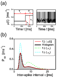
To estimate the ISI distribution in the complete stimulation period we assume that a given ISI of length was
either observed during the subinterval or the subinterval (see Fig. 1.a). This assumption constitutes an approximation, since in principle, an ISI can have its first spike in and the second one in . If and are sufficiently long, however, then the single ISI falling astride the two intervals can be neglected, compared to the numerous ISIs that lie entirely in one step or the other. The quasi-static approximation consists in assuming that the conditional probabilities of finding the ISI in each subinterval are equal to the stationary probabilities given by Eq. (2), with the corresponding values within each period (see Fig. 1.a). Notice that, again, this is not strictly true. Given that and are finite, boundary effects in the first and last ISIs could in principle modify the distribution.
In this context, we write
| (4) |
In this equation, weighs the probability of drawing ISIs from the interval . In addition, the probabilities and are
| (5) |
where is the expected number of ISIs in the -th subinterval, . Using Eq. (3) with to calculate we get
| (6) |
| (7) |
Eq. (7) implies that the overall density is a weighted average of the densities in each subinterval. In Fig. 1.b we show the histogram obtained from the simulation of Eq. (1) with the step-like input of Fig. 1.a, as well as the one obtained from the analytical expression, Eq. (7). Clearly, both densities agree.
II.3 Generalization to arbitrary time-dependent currents
Based on the quasi-static approximation, the result of the previous subsection can be extended to an arbitrary time-dependent input current. Suppose we make a partition of the stimulation period, {}, as shown in Fig. 2. The smooth positive function can be approximated by a sequence of constant strips, equal to the mean value of the function in each subinterval, {}. With this discrete partition, and proceeding as in the previous subsection, we obtain the ISI distribution valid for the complete stimulation period,
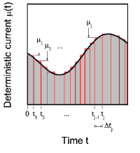
| (8) |
where . The partition can be inhomogeneous , for , and the functions are the stationary probability density of Eq. (2), for the particular values of the current within each subinterval. The continuum case is reached by making ,
| (9) |
Replacing in Eq. (9) by Eq. (2), the quasi-static ISI distribution in the entire stimulation period is
| (10) |
In the case of a two-step current, we averaged the distributions at each side of the jump, neglecting the single ISI that fell astride the two steps. In the case of continuous currents, in the limit of infinitesimal partitions, all ISIs fall on two or more partitions. The approximation, therefore, involves all ISIs. The procedure is justified when the stimulus varies only slightly inside each ISI. In this case, the input current since the last spike is essentially constant, and the approximation is expected to have a negligible effect.
Equation (10) is valid for PIF neurons with additive WGN of constant squared noise intensity . A similar argument can be used if also the noise intensity varies slowly in time. Since the noise intensity does not participate in the weighting factors, the extension of the previous result to this more general case is straightforward. In this case, we obtain
| (11) |
In summary, we have derived the ISI distribution of a PIF neuron valid in an extended stimulation period, when the input current (both signal and noise) vary slowly in time.
III Comparison to numerical data
We next test the validity of Eq. (10) for different input currents: linear, exponential, sinusoidal and Gaussian. We compare the analytical result with numerical simulations, to assess the validity of the quasi-static approximation. We show that the numerical and analytical distributions agree, when the stimulus varies slowly. As the time scale of stimulus variations becomes comparable to the mean ISI, the two results begin to differ.
III.0.1 Linear input current
A linear input current is defined by . Parameters and control the strength of the input, whereas the variation rate is determined by the length of the stimulation period .
For fixed , if decreases, the current varies faster.
The analytical expression given by Eq. (10) is integrable for linear currents, and the exact solution reads
| (12) |
Notice that the expression in Eq. (12) does not depend on the length of the stimulation period . Therefore, within the quasi-static approximation the ISI distribution only depends on the initial and final current values and . The total time taken to stimulate the neuron is irrelevant.
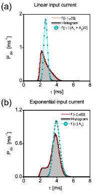
In Fig. 3.a we show the histogram obtained from the simulation of Eq. (1), and we compare it to the
probability density predicted by Eq. (12) for a large stimulation period, . The initial value of the membrane potential in different trials was randomly chosen between and , and ISIs were collected between the first and the last spikes within . The predicted ISI distribution agrees well with the real density. For comparison, we also show the density for a constant current equal to the arithmetic mean of and . Clearly, this distribution differs from the one obtained with a linear input current of the same mean.
For small , the input varies faster and the quasi-static approximation begins to fail. This occurs because of two reasons. In the first place, if at a given time the typical variation scale in the stimulus is smaller than the mean ISI, it is no longer true that the probability is well approximated by a constant current. In the second place, as the time before the first spike and the time after the last spike become comparable to the total interval , boundary effects are no longer negligible. In order to circumvent the impact of boundaries, the analysis of the failure of the quasi-static approximation is delayed to the case of sinusoidal stimulation (see below) where boundary effects are
negligible.
III.0.2 Exponential input current
The exponential current is defined by . Again, parameters and control the strength of the input, while defines the characteristic decay time. In this case, the explicit solution of the quasi-static expression Eq. (10) is not possible, so we resort to its numerical
integration (Simpson rule).
In Fig. 3.b we show the results for a large characteristic time . The total stimulation period was selected to be ten times the decay time . For even larger , the ISI distribution is dominated by the asymptotic value of the input. Again, the distribution obtained from the numerical simulation of Eq. (1) is in excellent agreement with the theoretical result of Eq. (10). We also show the density for the asymptotic constant current . The mismatch between this density and the real distribution shows that even for , the whole stimulus history influences .
III.0.3 Sinusoidal input current
The sinusoidal current is defined by . Numerical integration of Eq. (10) was used to obtain the quasi-static approximation for the ISI density. In this case, the characteristic time of variations in the stimulus is given by . Due to the periodicity of the input, the total stimulation time can be made arbitrarily long, thus minimizing boundary effects on the ISI distribution. Therefore, in this case, we can unambiguously explore the validity of the quasi-static approximation as the stimulus varies faster.
In Fig. 4.a we show the quasi-static ISI distribution and we compare it to the histogram constructed from simulations for a slow driving frequency (), and a large total stimulation period equal to a finite number of cycles (). Clearly, both distributions agree. For comparison, we also show the density for a constant input, with . Notably, the density for the mean value is completely different from the real distribution.
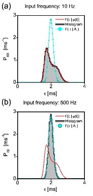
As the input frequency increases, the quasi-static approximation Eq. (10) begins to depart from the real ISI distribution. In Fig. 4.b we show a faster sinusoidal current with (). With this input, the real and the quasi-static densities are noticeable different, and actually the real distribution gets closer to the mean constant input density. Crudely, a fast oscillatory current produces a similar effect to that of a constant mean current, with higher noise amplitude.
III.0.4 Noisy Gaussian input currents
Finally, we test the quasi-static approximation with a more irregular input, as done previously for example in lansky2008 . In our case, the stimulus consists of a Gaussian signal with a sharp cutoff frequency . Similarly to the case of sinusoidal current, we denote the mean and the standard deviation of the signal in the temporal domain by and , respectively. These parameters control the strength of the input.
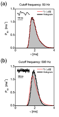
In particular, we tested two stimuli with different cutoff frequencies: and , respectively. As shown in the insets of Fig. 5, the signal with the higher cutoff frequency displays more rapid fluctuations. In Fig. 5.a we see the ISI distributions from both the simulation of Eq. (1) and the quasi-static approximation Eq. (10), for . The agreement between the two distributions is excellent. As the signal fluctuates more rapidly, the quasi-static approximation for the ISI distribution starts to deviate from the real behavior. Fig. 5.b shows the distributions for a stimulus of . In this case, the quasi-static approximation is no longer applicable.
IV Discussion and Conclusions
In this paper, we use a quasi-static approximation to derive the ISI distribution of a PIF neuron driven by a time-dependent input current. Different temporal dependencies were used to test the approximation. Linear currents were employed first, since they allow an analytic integration of the ISI distribution. Currents with other temporal dependencies required the numerical integration of Eq. (10). Exponential input currents are a realistic description of adaptation currents in the brain benda2003 . Sinusoidal stimuli represent periodic collective oscillations, as for example, the theta rhythm in hippocampus. Random low-passed Gaussian driving is an approximation to the LFP in sensory cortices. In all cases, for slowly varying stimuli, an excellent agreement between the theoretical ISI distribution and the one obtained by simulating the dynamical equations was achieved. As expected, when the stimulus varies in time-scales comparable to the ISIs themselves, the approximation begins to fail.
In previous studies, sinusoidal input currents were classified as either endogenous or exogenous lansky1997 . Exogenous stimuli are external signals, that do not depend on the activity of the neuron under study. Endogenous inputs, in contrast, are instantaneously reset to a particular phase, every time the cell generates a spike. Endogenous signals are more convenient for mathematical manipulations bulsara1994 . However, as discussed in plesser2001 , they do not
constitute a realistic description of external sensory or synaptic input. They can only be justified in the subthreshold, noise-driven regime, where spike generation is only possible in specific stimulus phases. In this regime, neuronal dynamics is characterized by a typical time scale, associated to the average time required by the input noise to drive the cell across threshold. When this time scale is an integer multiple of the period of the sinusoidal input current, stochastic resonance and multi peaked ISI distributions are obtained bulsara1994 ; plesser2001 ; bulsara1996 ; plesser1997 ; plesser1999 ; shimokawa1999 ; shimokawa2000 ; schindler2004 ; kostur2007 . In this paper, however, we have focused on positive currents , which mimic the supra-threshold regime of leaky integrate-and-fire neurons. In this regime, the drift current term is sufficient to generate firing. Input noise randomizes the process of spike generation, introducing spike-time jitter, but does not determine a characteristic waiting interval. Therefore, there is no noise-dependent escape time and the multi peaked ISI distributions characteristic of stochastic resonance are not observed.
The basic formulas of this paper Eqs. (10) to (12) are only valid for the PIF neuron. However, extensions to other neuron models can be developed. To that end, one needs to know how depends on the input strength (and possibly ), to be able to derive a relation analogous to Eq. (6). In addition,
must be known, in order to further proceed to Eq. (10) or Eq. (11). Therefore, the approach we pose in this paper could also be applied in other areas. For example, in an impressive modelling work about the nature of the ion channel gating, Goychuk and Hänggi developed a stochastic microscopic description of the transition from closed to open conformations of potassium channels goychuk2002 . In their model, the authors posed the problem in the Fokker-Planck formalism and argued for appropriate boundary conditions. They explicitly solved the residence time distribution in the Laplace domain and obtained the “unusual” opening rate of this kind of channels. One of the key points in their analysis is that the activation rate depends on a potential (describing the conformational energy barrier), which in turn depends on the voltage. However, in real conditions this voltage depends on time, since the extracellular environment surrounding any central neuron is modulated by the collective LFP. The Fokker-Planck formalism used in goychuk2002 can also be phrased within the Langevin approach used in our work. Thus, our method could be useful to extend their results to time-modulated potentials. This example shows the broad applicability of the quasi-static formulation.
The knowledge of the ISI distribution obtained for time-dependent stimuli is useful to assess the effect of an evolving current in the firing dynamics of a neuron. This distribution characterizes the running rate code, as received by a downstream target: if the post-synaptic neuron has a fairly long integration time, the statistics of ISIs received during the integration interval depend on the evolution of the stimulus inside that period. In addition, in the quasi-static limit, the ISI distribution can also be used to calculate mutual information rates zador1998 .
References
- (1) H. L. Bryant, and J. P. Segundo, J. Physiol. 260, 279 (1976).
- (2) Z. F. Mainen and T. J. Sejnowski, Science 268, 1503 (1995).
- (3) G. Buzsáki, Rhythms of the brain, (Oxford University Press, New York, 2006).
- (4) K. Tóth, T. F. Freund, and R. Miles, J. Physiol. 500, 463 (1997).
- (5) A. Fontanini, and J. M. Bower, Trends Neurosci. 29, 429 (2006).
- (6) P. Berens, G. A. Keliris, A. S. Ecker, N. K. Logothetis, and A. S. Tolias, Front. Syst. Neurosci. 2), 1 (2008).
- (7) C. B. Saper, Brain stem modulation of sensation, movement and consciousness, 889, in Principles of neural science (4th ed.), edited by E. R. Kandel, J. H. Schwartz, and T. M. Jessell (McGraw-Hill, New York, 2000).
- (8) K. Doya, Neural Networks 15, 495 (2002).
- (9) E. Marder, Modulating neural properties of neurons: role in information processing, in Exploring Brain Functions: Models in Neuroscience, edited by T. A. Poggio, and D. A. Glaser (John Wiley & Sons Ltd., New York, 1993).
- (10) P. S. Katz, Current Opinion in Neurobiology. 5, 799 (1995).
- (11) M. P. Nusbaum, and M. P. Beenhakker, Nature 417, 343 (2002).
- (12) B. Ermentrout, Neural Comput. 10, 1721 (1998).
- (13) J. Benda, and A. V. M. Herz, Neural Comput. 15, 2523 (2003).
- (14) P. Sah, Trends Neurosci. 19, 150 (1996).
- (15) F. Helmchen, K. Imoto, and B. Sakmann, Biophys. J. 70, 1069 (1996).
- (16) C. J. Wilson, A. Weyrick, D. Terman, N. E. Hallworth, and M. D. Bevan, J. Neurophysiol. 91, 1963 (2004).
- (17) A. N. Burkitt, Biol. Cybern. 95, 1 (2006).
- (18) A. N. Burkitt, Biol. Cybern. 95, 97 (2006).
- (19) W. Kistler, W. Gerstner, and J. L. van Hemmen, Neural Comput. 9, 1015 (1997).
- (20) H. C. Tuckwell, Introduction to Theoretical Neurobiology, (Cambridge University Press, Cambridge, 1988).
- (21) W. Gerstner, and W. Kistler, Spiking Neuron Models: Single Neurons, Populations, Plasticity, (Cambridge University Press, Cambridge, 2002).
- (22) A. Aldo Faisal, L. P. J. Selen, and D. M. Wolpert, Nat. Rev. Neurosci. 9, 292 (2008).
- (23) M. E. Larkum, W. Senn, and H. -R. Lüscher, Cer. Cortex 14, 1059 (2004).
- (24) J. A. White, J. T. Rubinstein, and A. R. Kay, Trends Neurosci. 23, 131 (2000).
- (25) E. Schneidman, B. Freedman, and I. Segev, Neural Comput. 10, 1679 (1998).
- (26) G. A. Jacobson, K. Diba, A. Y. -Jakoubovitch, Y. Oz, C. Koch, I. Segev, and Y. Yarom, J. Physiol. 564, 145 (2005).
- (27) A. Zador, J. Neurophysiol. 79, 1219 (1998).
- (28) M. London, A. Schreibman, M. Häusser, M. E. Larkum, and I. Segev, Nat. Neurosci. 5, 332 (2002).
- (29) W. Bialek, and S. Setayeshgar, Proc. Natl. Acad. Sci. USA 102, 10040 (2005).
- (30) G. L. Gerstein and B. Mandelbrot, Biophys. J. 4, 41 (1964).
- (31) P. Lánský, and L. Sacerdote, Phys. Lett. A 285, 132 (2001).
- (32) U. Picchini, S. Ditlevsen, A. De Gaetano, and P. Lánský, Neural Comput. 20, 2696-2714 (2008).
- (33) P. Lánský, Phys. Rev. E 55, 2040 (1997).
- (34) A. R. Bulsara, S. B. Lowen, and C. D. Rees, Phys. Rev. E 49, 4989 (1994).
- (35) H. E. Plesser, and T. Geisel, Phys. Rev. E 63, 031916 (2001).
- (36) A. R. Bulsara, T. C. Elston, C. R. Doering, S. B. Lowen, and K. Lindenberg, Phys. Rev. E 53, 3958 (1996).
- (37) H. E. Plesser, and S. Tanaka, Phys. Lett. A 225, 228 (1997).
- (38) H. E. Plesser, and T. Geisel, Phys. Rev. E 59, 7008 (1999).
- (39) T. Shimokawa, K. Pakdaman, and S. Sato, Phys. Rev. E 59, 3427 (1999).
- (40) T. Shimokawa, K. Pakdaman, T. Takahata, S. Tanabe, and S. Sato, Biol. Cybern. 83, 327 (2000).
- (41) M. Schindler, P. Talkner, and P. Hänggi, Phys. Rev. Lett. 93, 048102 (2004).
- (42) M. Kostur, M. Schindler, P. Talkner, and P. Hänggi, Math. Biosci. 207, 302 (2007).
- (43) I. Goychuk, and P. Hänggi, Proc. Natl. Acad. Sci. USA 99, 3552-3556 (2002).