An observation regarding systems which converge to steady states
for all constant inputs, yet become chaotic with periodic inputs

Abstract

This note provides a general construction, and gives a concrete example of, forced ordinary differential equation systems that have these two properties: (a) for each constant input $u$, all solutions converge to a steady state but (b) for some periodic inputs, the system has arbitrary (for example, “chaotic”) behavior. An alternative example has the property that all solutions converge to the same state (independently of initial conditions as well as input, so long as it is constant).

1 The question

We consider systems

$$\dot{x}(t)=f(x(t),u(t))$$

of forced ordinary differential equations, where $u=u(t)$ is an input, assumed scalar-valued for simplicity.

It is well-known fact that a system that exhibits periodic trajectories when unforced may well exhibit chaotic behavior when forced by a periodic signal, as shown by Van der Pol equations with nonlinear damping, and nonlinear-force Duffing systems. However, the following fact seems to be less appreciated.

Assume that the system has the property that, whenever $u(t)$ is constant (any value), all solutions converge to a steady state (which might depend on the input and on the initial conditions). Is it possible for such a system to behave pathologically with respect to periodic inputs (no “entrainment”)? We outline a general construction together with a specific example of this phenomenon.

A second construction is also given, which has the property that all solutions for constant inputs converge to the same state (independently of initial conditions as well as the input value, so long as it is constant). This second construction displays a more interesting phenomenon, but it is only done for an example (Lorentz attractor), and it seems difficult to prove rigorously that its solutions when forced by a periodic input are truly chaotic.

2 The general construction

The general construction is illustrated in Figure 1.

Figure 1: General construction

The block called “filter 1” consists of a linear system $\dot{x}=Ax+Bu$ with output $y=Cx+Du$ having the property that its transfer function $W(s)$ (the Laplace transform of the impulse response $Ce^{tA}B$) is not identically zero but has a zero at the origin: $W(0)=0$.

The differentiable function $\alpha:{\mathbb{R}}\rightarrow{\mathbb{R}}_{\geq 0}$ has the property that $\alpha(0)=0$ but $w(t)=\alpha(y(t))$ saturates at the value $1$ if $y(t)$ is outside a small neighborhood of zero.

The block called “filter 2” consists of a scalar linear system $\dot{p}=-p+w$. If the signal $w(t)$ converges to zero, then $p(t)$ also converges to zero. However, if the signal $w(t)\approx 1$ for a large set of times $t$, then $p(t)$ will, after a transient, stay always positive and bounded away from zero, through an averaging effect.

Finally, the block named “system” has the form $\dot{z}(t)=p(t)f(z(t))$, where $f$ is an arbitrary vector field with bounded solutions. Provided that the scalar signal $p(t)$ remains positive and bounded away from zero, the solutions of the system will be time-rescaled versions of solutions of $\dot{z}=f(z)$, and hence have the same pathologies.

When the input $u(t)$ is constant, the fact that the transfer function vanishes at zero means that $y(t)\rightarrow 0$ as $t\rightarrow\infty$. This implies that $w(t)\rightarrow 0$, and so $p(t)\rightarrow 0$ as well. Thus the velocity $\dot{z}(t)\rightarrow 0$, and solutions become asymptotically constant.

On the other hand, suppose that the input is $u(t)=\sin\omega t$, where $W(i\omega)\not=0$. This means that the output $y(t)$ will be asymptotically of the form $A\sin(\omega t+\varphi)$, for some phase $\varphi\in{\mathbb{R}}$ and some amplitude $A=\left|W(i\omega)\right|\not=0$. Assuming that $A$ is large enough, passing $y(t)$ through $\alpha$ will result in a signal $w$ that is mostly saturated near the value $1$, so $p(t)$ will stay away from zero and the solutions of the $z$ subsystem will look (asymptotically) like those of $\dot{z}=f(z)$.

3 An explicit example

Let us take “filter 1” to be the system $\dot{x}=-x-u$ with output $y=x+u$, the function $\alpha(y)=y^{2}/(K+y^{2})$ with $K=1/10$, and the vector field corresponding to the Lorentz attractor with parameters in the chaotic regime. Specifically, the complete system is as follows.

$$\dot{x} = -x-u$$

$$\dot{p} = -p+\alpha(x+u)$$

$$\dot{\xi} = p(s(\psi-\xi))$$

$$\dot{\psi} = p(r\xi-\psi-\xi\zeta)$$

$$\dot{\zeta} = p(\xi\psi-b\zeta)$$

with Prandtl number $s=10$, Rayleigh number $r=28$, and $b=8/3$. Figure 2 shows typical solutions of this system with a periodic and constant input respectively.

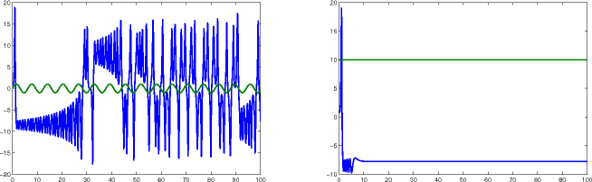
Figure 2: Some solutions of example system. Initial conditions are $x(0)=5$, $\xi(0)=1$, and all remaining variables zero. Green: inputs are $u(t)=\sin t$ (left panel) and $u(t)=10$ (right panel). Blue: $\xi(t)$. Note chaotic-like behavior in response to periodic input, but steady state in response to constant input.

4 An alternative example

Instead of multiplying the Lorentz vector field by $p(t)$, we may use $p(t)$ to eliminate the multiplicative terms, making the system asymptotically linear and time-invariant, and also changing one of the coefficients in such a way that the corresponding linear system is globally asymptotically stable. Simulations (using a Montecarlo sampling of initial conditions as well as input magnitudes) indicate that the system remains chaotic when forced by $\sin t$, but all solutions converge to zero when $u(t)$ is constant. Specifically, the complete system is as follows.

$$\dot{x} = -x-u$$

$$\dot{p} = -p+\alpha(x+u)$$

$$\dot{\xi} = 10(\psi-\xi)$$

$$\dot{\psi} = 28p\xi-\psi-p\xi\zeta$$

$$\dot{\zeta} = p\xi\psi-(8/3)\zeta$$

Observe that when $p=0$ one has, for the last three variables, the stable linear system:

$$\dot{\xi} = 10(\psi-\xi)$$

$$\dot{\psi} = -\psi$$

$$\dot{\zeta} = -(8/3)\zeta$$

and when $p=1$ the system is the usual Lorentz attractor

$$\dot{\xi} = 10(\psi-\xi)$$

$$\dot{\psi} = 28\xi-\psi-\xi\zeta$$

$$\dot{\zeta} = \xi\psi-(8/3)\zeta\,.$$

In order to achieve $p\approx 1$ for the input $\sin t$, we now pick $K=0.0001$ in the definition of $\alpha$. Figure 3 shows typical solutions of this system with a periodic and constant input respectively. The function “rand” was used in MATLAB to produce random values in the range $[-10,10]$.

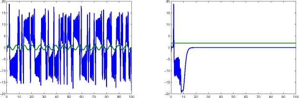
Figure 3: Simulation of second example, done with the following randomly-chosen input and initial conditions: $u(t)=1.89$, $x(0)=2.95$ $p(0)=-0.98$, $\xi(0)=0.94$, $\psi(0)=-4.07$, $\zeta(0)=4.89$. Green: inputs are $u(t)=\sin t$ (left panel) and $u(t)=5.13$ (randomly picked, right panel). Blue: $\xi(t)$. Note chaotic-like behavior in response to periodic input, but steady state in response to constant input.

To better understand the behavior of this system, Figure 4 shows the value of the input and the variable $p(t)$, for the same input and initial conditions as in Figure 3.

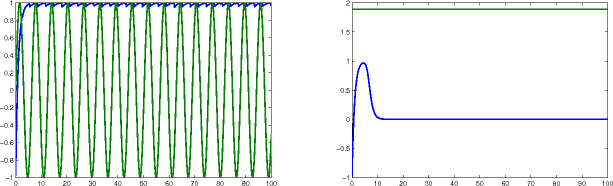
Figure 4: Inputs and variable $p(t)$ for simulation shown in Figure 4. Note that $p(t)\approx 1$ and $p(t)\approx 0$ for $t\gg 0$.

5 Remark

One could clearly extend the construction to “interpolate” between any two dynamics: using $\dot{z}(t)=p(t)f_{1}(z(t))+(1-p(t))f_{0}(z(t))$ means that, for constant inputs, asymptotically the system will behave like $\dot{z}=f_{0}(z(t))$, while for $u(t)=\sin t$ it will behave like $\dot{z}=f_{1}(z(t))$. Establishing a precise result in this generality would require a detailed study of chain-recurrent sets and other objects associated to asymptotically autonomous dynamics. We leave that to future work.