Calculation of Atomic Number States: a Bethe Ansatz Approach

Abstract

We analyze the conditions for producing atomic number states in a one-dimensional optical box using the Bethe ansatz method. This approach provides a general framework, enabling the study of number state production over a wide range of realistic experimental parameters.

I Introduction

The realization of Bose-Einstein condensation (BEC) in dilute gases has enabled the study and control of many-body systems. While most of the work has focused on the properties and excitations of the condensate, it has provided a new path towards generation of atomic number (or Fock) states. These few body states with a definite number of atoms in the ground state are of great interest for quantum information where individual qubits can be addressed Dudarev:2003 ; Jaksch:1999 ; Andersson:2000 , and could also be important for atom interferometry in order to reach the Heisenberg limit of detection. Experimentally, realization of Fock states requires a BEC confined in an optical box coupled with single-atom counting. The challenge is to obtain confinement in a trap that is comparable to optical lattices, but with only a single site Meyrath:2005 . Recent experimental work has demonstrated all the necessary steps towards this goal and they are now being incorporated into a single system Chuu:2005 . In parallel, the theoretical analysis of this problem has focused on the conditions for optimum number state production Dudarev:2007 ; ACampo:2008-2009 . These include the role of varying trap depth and size, either separately or in tandem. The interaction strength is a third control parameter that can be tuned with the the help of Feshbach resonances or by tuning the transverse confinement of the optical trap Meyrath:2005 ; Inouye:1998 and is considered here in more detail.

It is clear that strong repulsion between atoms are desirable for the production of number states. The infinitely strong interaction regime is the so-called Tonks-Girardeau regime where calculation has been made trivial thanks to the boson-fermion correspondence Girardeau:1960 . However, this is only an unreachable limiting case. To make realistic predictions about what can be experimentally realized, we must consider the regime of relatively but not infinitely strong interactions. Previous studies of this regime were carried out using numerical methods which are both time-consuming and reveal little insight on how number states vary with interaction strength. In this paper we develop an approach that takes interaction as a parameter and by which we are able to chart number states in the parameter space with interaction as one of its dimensions comment1 .

Our analysis of the production of atomic number states in a 1D optical box is based on the so-called Bethe ansatz approach. This method was first developed by Hans Bethe to solve the problem of a one-dimensional (1D) spin 1/2 Heisenberg ferromagnet Bethe:1931 . Since it’s invention, Bethe’s method has found important applications in the study of interacting spin systems Orbach:1958 ; Walker:1959 ; Lieb:Schultz:Mattis:1961 . It has also been applied to solve the problem of a 1D bosonic gas with repulsive $\delta$-function interactions Lieb:Liniger:1963 ; McGuire:1964 ; Yang:1967 ; Gaudin:1967 ; Sutherland:1968 ; Li:1995 ; Hao:2006 . An outline for the structure of this article is as follows. In section II, we formulate the problem; in section III, we present approximate solutions to our problem with Bethe ansatz approach; in section IV, we use Bethe ansatz solutions to analyze issues related to number state production.

II Formulation of the problem

The problem of many bosons with a $\delta$-function interaction trapped in 1D square well potential with finite well depth was studied using the Bethe ansatz in Ref Li:1995 . We find the problem of producing Fock states in the ultracold atom systems trapped in 1D optical box bears similar characteristics. We treat the 1D optical trap as a square well potential of length $L$ and depth $V_{0}$. We write the interaction potential as $\frac{\hbar^{2}}{m}c\delta(x_{i}-x_{j})$, where $x_{i}$ and $x_{j}$ are the positions of the interacting particles, $\hbar$ is Planck’s constant and $m$ is an atom’s mass, and $c$ is the interaction strength and has dimension of $[1/\mbox{length}]$. According to Olshanii:1998 we have the following expression for $c$,

$$c=\frac{4a}{{a_{\perp}}^{2}}\left(1-C\frac{a}{a_{\bot}}\right)^{-1},$$ (1)

where $a$ is the s-wave scattering length in 3-dimensional space, $a_{\perp}=\sqrt{{2\hbar^{2}}/m\omega_{\perp}}$, $\omega_{\perp}$ is the transverse trapping frequency, and $C\approx 1.4603$ is an empirical constant number. Since the interaction strength $c$ depends on both scattering length and transverse trapping frequency $\omega_{\perp}$, tuning either of them will affect the interaction strength. The transverse trapping frequency may be controlled by optical box parameters Meyrath:2005 . Scattering length may be adjusted by Feshbach resonance Inouye:1998 . To give a sense of order of magnitude, for sodium atoms trapped in a 1D optical box with transverse trapping frequency $\omega_{\perp}=2\pi\times 150$ kHz and zero magnetic field, we have $c=16863.6\mbox{ cm}^{-1}$. For ⁸⁷Rb atoms in a similar trap with zero magnetic field, we have $c=92391.6\mbox{ cm}^{-1}$.

To make our equations dimensionless, we use $1/c$ as the length unit and $\hbar^{2}c^{2}/m$ as the energy unit. The square well potential is then

$$V\left(x\right)=\left\{\begin{array}[]{cc}-{k_{0}}^{2}/2,&|x|<x_{0}/2,\\ 0,&\mbox{ otherwise},\\ \end{array}\right.$$ (2)

where $k_{0}$ and $x_{0}$ are dimensionless numbers. With these parameters, the well width is $L=x_{0}/c$ and well depth is $V_{0}=\hbar^{2}c^{2}{k_{0}}^{2}/2m$ in cgs unit.

The hamiltonian for the many-body system may be written as

$${\mathcal{H}}=-\frac{1}{2}\sum_{i=1}^{N}{\frac{\partial^{2}}{\partial x_{i}^{2}}}+\sum_{i=1}^{N}{V\left(x_{i}\right)}+\mathop{\sum_{i,j=1}^{N}}_{i>j}{\delta\left(x_{i}-x_{j}\right)}.$$ (3)

Our first main step is to solve the following eigenvalue problem

$${\mathcal{H}}\psi(\overrightarrow{x})=E\psi(\overrightarrow{x}),$$ (4)

where $\overrightarrow{x}$ is shorthand for $x_{1},x_{2},\cdots,x_{N}$. We are primarily interested in bound states whose wavefunctions must be normalizable. As a minimum requirement, the wavefunction of a bound state must satisfy $\lim_{x\to\pm\infty}{\psi(\overrightarrow{x})}=0$.

III Bethe Ansatz solutions

In section II, we defined a boundary value problem relevant to the production of number states. We will in this section apply Bethe ansatz and obtain solutions for it.

As studied in previous literatures Li:1995 ; Yang:1967 ; Lieb:Liniger:1963 , Bethe ansatz solution of this problem introduces a set of $N$ as-yet-unknown wave numbers $\overrightarrow{k}=\{k_{1},k_{2},\cdots,k_{N}\}$. In conjugate to these wave numbers, another set $\overrightarrow{\kappa}=\{\kappa_{1},\kappa_{2},\cdots,\kappa_{N}\}$ is defined as

$$\kappa_{j}=\sqrt{k_{0}^{2}-{k_{j}}^{2}},$$ (5)

for $j=1,2,\cdots,N$. The total energy of the Bethe ansatz state is $E=-\sum_{j}^{N}{{\kappa_{j}}^{2}/2}=\sum_{j}^{N}{\left({k_{j}}^{2}-{k_{0}}^{2}\right)/2}$. The eigenfunction (wavefunction) of Eq.(4) is piecewise continuous in the $N$-dimensional coordinate space $\{x_{1},x_{2},\cdots,x_{N}\}$. For simplicity, we consider three representative regions in the $N$-dimensional coordinate space:

$$R_{1} : -x_{0}/2<x_{1}<x_{2}<\cdots<x_{N}<x_{0}/2,$$ (6)

$$R_{2} : x_{1}<-x_{0}/2<x_{2}<\cdots<x_{N}<x_{0}/2,$$ (7)

$$R_{3} : -x_{0}/2<x_{1}<\cdots<x_{N-1}<x_{0}/2<x_{N}.$$ (8)

$R_{1}$ represents a region where all particles are trapped; $R_{2,(3)}$ represent a region where the $1$st ($N$th) particle tunnels into the left (right) barrier. In fact, each of these regions falls in a class consisting of $N!$ regions that are related by coordinate permutation. For ease of reference, we name $\mathcal{A}$ the class of regions that can be obtained from $R_{1}$ by mere coordinate permutations and study the wavefunctions in these regions at once.

We denote the wavefunctions in a region of $\mathcal{A}$ as $\phi_{\tau}(\overrightarrow{x})$, where $\tau$ is the permutation operator that transforms $R_{1}$ into this region, i.e., $R_{\tau}=\tau R_{1}$. This wavefunction is the superposition of pure plane waves with “$\pm$ signs” times permuted wave numbers,

$$\phi_{\mathbf{\tau}}(\overrightarrow{x})=\sum_{\varsigma\in C_{2}^{N}}{\sum_{\mathbf{\sigma}\in\mathbf{G}}{A\left(\varsigma,\sigma;\mathbf{\tau}\right)e^{i(\varsigma\mathbf{\sigma}\overrightarrow{k})\cdot\overrightarrow{x}}}}.$$ (9)

where $\varsigma\equiv\left\{\varsigma_{1},\varsigma_{2},\cdots,\varsigma_{N}\right\}$ represents a possible combination of $N$ signs each of which is either $+$ or $-$ and $C_{2}^{N}$ represents the group of such operations, $\mathbf{G}$ is the permutation group of $N$ particles, and $A(\varsigma,\mathbf{\sigma};\tau)$ is the superposition amplitude.

It is clear that the superposition amplitude $A(\varsigma,\mathbf{\sigma};\mathbf{\tau})$ is a functional of the sign-flipping operator, the wave number permutation operator, and the region permutation operator. By bosonic particle permutation symmetry, we establish the first set of equations among the superposition amplitudes,

$$A(\varsigma,\mathbf{\sigma};\mathbf{\tau})=A(\varsigma,\mathbf{\tau\sigma};\mathbf{I}),$$ (10)

where $\mathbf{I}$ is the identity element in the permutation group.

The wavefunctions in region $R_{2}$ have a more complicated form,

$$\phi_{2}(\overrightarrow{x})=\sum_{\varsigma}{\sum_{\mathbf{\sigma}\in\mathbf{G}}{B(\varsigma,\mathbf{\sigma})e^{{(\mathbf{\sigma}\overrightarrow{\kappa})}_{1}x_{1}}e^{i\sum_{j=2}^{N}{(\mathbf{\varsigma\sigma}\overrightarrow{k})_{j}x_{j}}}}},$$ (11)

where $(\mathbf{\varsigma\sigma}\overrightarrow{k})_{j}$ is the $j$th component wave number after the permutation operation $\sigma$ and the sign-flipping operation $\varsigma$, ${(\mathbf{\sigma}\overrightarrow{\kappa})}_{1}\equiv\sqrt{k_{0}^{2}-{(\mathbf{\sigma}\overrightarrow{k})_{1}}^{2}}$, which can be regarded as an extra operator on top of the permutation operator $\mathbf{\sigma}$, and $B(\mathbf{\varsigma,\sigma})$ is the superposition amplitude. Similarly, the wavefunctions in region $R_{3}$ may be written as,

$$\phi_{3}(\overrightarrow{x})=\sum_{\varsigma}{\sum_{\mathbf{\sigma}\in\mathbf{G}}{C(\mathbf{\varsigma,\sigma})e^{i\sum_{j=1}^{N-1}{(\varsigma\sigma\overrightarrow{k})_{j}x_{j}}}e^{-(\mathbf{\sigma}\overrightarrow{\kappa})_{N}x_{N}}}},$$ (12)

where ${(\mathbf{\sigma}\overrightarrow{\kappa})}_{N}\equiv\sqrt{k_{0}^{2}-{(\mathbf{\sigma}\overrightarrow{k})_{N}}^{2}}$ and $C(\mathbf{\varsigma,\sigma})$ is the superposition amplitude.

From Eq.(5), it is clear that if, for any i, $k_{i}>k_{0}$ then there will be a corresponding pure imaginary $\kappa_{i}$. From Eq.(11), Eq.(12), any pure imaginary $\kappa_{i}$ will cause the Bethe ansatz wavefunction unnormalizable. Then from the normalizability requirement stated at the end of Section I, we reason that a Bethe ansatz state is bound if and only if all of the wave numbers are real and smaller than $k_{0}$. Since we are primarily interested in bound states, from now on we implicitly mean bound state when we say Bethe ansatz state, unless otherwise stated.

Once we get the Bethe ansatz wavefunctions written down, the rest is straightforward. The main features of Eq. (4) are the singular $\delta$-function particle-particle interaction and the nonzero potential step at the edge of the square well. Bethe ansatz method elegantly treats both as boundary conditions. The boundary conditions at $x_{i}-x_{j}=0$ for $i,j=1,2,\cdots,N$ in regions of class $\mathcal{A}$ requires continuity of wavefunctions on the one hand,

$$\left.\psi\right|_{x_{i}={x_{j}}^{+}}=\left.\psi\right|_{x_{i}={x_{j}}^{-}}$$ (13)

and certain discontinuity in their first-derivatives on the other,

$$\left.\left[\frac{\partial\psi}{\partial x_{i}}-\frac{\partial\psi}{\partial x_{j}}\right]\right|_{x_{i}={x_{j}}^{+}}-\left.\left[\frac{\partial\psi}{\partial x_{i}}-\frac{\partial\psi}{\partial x_{j}}\right]\right|_{x_{i}={x_{j}}^{-}}=2c\left.\psi\right|_{x_{i}=x_{j}}.$$ (14)

The boundary conditions at $x_{i}=\pm x_{0}/2,i=1,2,\cdots,N$ require continuity of both wavefunctions and their first-derivatives:

$$\left.\psi\right|_{x_{i}={x_{0}/2}^{+}} = \left.\psi\right|_{x_{i}={x_{0}/2}^{-}}$$ (15)

$$\left.\frac{\partial\psi}{\partial x_{i}}\right|_{x_{i}={x_{0}/2}^{+}} = \left.\frac{\partial\psi}{\partial x_{i}}\right|_{x_{i}={x_{0}/2}^{-}}.$$ (16)

Plugging Eq.(9), (11), and (12) into Eq.(13), (14), (15), and (16) and including Eq.(10), we obtain the complete group of equations for our original problem.

For the purpose of this article, it suffices to keep just the wave numbers and eliminate all other unknowns. Doing so yields the following secular equations for the $N$ wave numbers,

$$-x_{0}k_{j}=-\pi I_{j}+2\sin^{-1}{\left(\frac{k_{j}}{k_{0}}\right)}+$$ (17)

$$+\sum_{l=1,l\neq j}^{N}{\left[\tan^{-1}{\left({k_{j}+k_{l}}\right)}+\tan^{-1}{\left({k_{j}-k_{l}}\right)}\right]},$$

where $j=1,2,\cdots,N$, and $I=\{I_{1},I_{2},\cdots,I_{N}\}$ is a set of preselected integers.

Now a retrospect on the three regions we selected in the coordinate space might make you wonder why we haven’t included more regions (and more equations), possibly with 2 or more particles lying outside the trap area simultaneously. In reality, this is possible, but only with small probability for deeply bound state. The effect on the number-state condition should be ignorable. Firstly, insofar as representative limiting cases (strong interaction limit and deep trap limit), Bethe ansatz solution agrees with known results (see Fig. 2a). Secondly, the energy spacings between single-particle levels are big near the strong interaction regime where number state experiments take place most likely and therefore the probability for more than one particle to tunnel into the barrier is ignorably small at all times. For this reason, we argue that the Bethe ansatz-based approach is a sufficiently good approximation to our problem.

There are a few notable aspects of Eq. (17). Firstly it is a transcendental equation and so does not have analytic solution. Secondly, we must pick a set of integers $I=\{I_{1},I_{2},\cdots,I_{N}\}$ before we start the numerical computation. Apparently, not any set of integers would lead to a physically meaningful solution. Then a natural question to ask is what does. As argued in Appendix A, we find that Eq. (17) yield valid solution if and only if the set of integers $I$ are mutually distinct, somewhat similar to the theorem in Ref. Yang:1967 . A corollary of is that wave numbers thus obtained have mutually distinct absolute values. Because of this one-one correspondence, we use the set $I$ as the quantum numbers for the corresponding Bethe ansatz state.

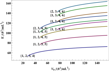
Figure 1: (color online) Bethe ansatz states for sodium atoms. The total energy of 4-particle bound states are plotted against trap depth. The numbers at the beginning of each energy level are the quantum numbers of the bound state. We shifted the energy zero to the bottom of the trap for ease of presentation. Trap size $L=5\mbox{ }\mu$m. Transverse trapping frequency $\omega_{\perp}=2\pi\times 150$ kHz.

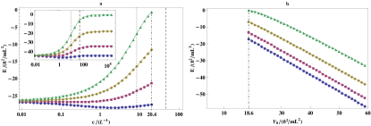
Figure 2: (color online) Single particle energies of $4$ sodium atoms in Bethe ansatz ground states. Trap size $L=5\mu$m. a. Dependence on interaction strengths ($c$). Trap depth $V_{0}=k_{B}\times 25$nK, where $k_{B}$ is Boltzmann’s constant. The dotdashed vertical line denotes the maximum interaction strength above which no Bethe ansatz state of 4-boson system exists. The other two vertical lines denote the interaction strengths of sodium (dotted) and ⁸⁷Rb (dashed) atoms at $\omega_{\perp}=2\pi\times 150$ kHz and zero magnetic field. Inset, the trap depth is lifted to $k_{B}\times 40$nK, at which condition all 4 atoms remain trapped to the Tonks limit. b. Dependence on trap depths ($V_{0}$). Transverse trapping frequency $\omega_{\perp}=2\pi\times 150$ kHz. Magnetic field is zero. The vertical line (dotdashed) denotes the minimum trap depth below which no bound state of 4-boson system exists.

Besides knowing what set of integers are valid quantum numbers, we need further identify the ground state and the first-excited state. As argued in Appendix B, we find that the ground state of an $N$-boson system has the quantum number $\{1,2,\cdots,N\}$; the first-excited state has the quantum number $\{1,2,\cdots,N-1,N+1\}$ (see Fig. 1).

Without loss of generality, we re-organize the set of wave numbers such that $0<k_{1}<k_{2}<\cdots<k_{N}<k_{0}$. We define the $j$th single particle energy as $e_{j}=-{\kappa_{j}}^{2}/2$, for $j=1,2,\cdots,N$. Fig. 1 gives total energies of the low-lying Bethe ansatz states.

IV Number states

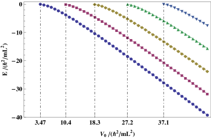
Figure 3: (color online) Ionization thresholds of sodium atoms with all parameters fixed except trap depth (we use $\hbar^{2}/mL^{2}$ as energy unit for convenience). Only highest single particle energies of the Bethe ansatz $N$-boson states are shown with $N=$ 2 (circle), 3 (square), 4 (diamond), 5 (upright triangle), and 6 (invert triangle). Trap size $L=5\mbox{ }\mu$m; Transverse trapping frequency $\omega_{\perp}=2\pi\times 150$ kHz. The ionization thresholds (with the current numeric calculation step size) are marked with vertical lines (dot-dashed).

We now apply the results of the previous sections to the problem of number state production. We can safely assume no atom with positive energy presents in space near the trapped area. In reality, if an atom acquires positive energy, it would be quickly swept out of the vacuum chamber. Therefore, it is safe to assume that the states in the continuum spectrum are virtually unoccupied all the time.

As dictated by Bethe ansatz, for some given trap parameters (depth $V_{0}$, trap size $L$, scattering length $a$, and transverse trapping frequency $\omega_{\perp}$), $N$ bosons can be contained in the trap if and only if there is an $N$-boson Bethe ansatz state. The energy levels for an $N$-boson system has been computed by Eq.(17) numerically. As an example, Fig. 2 shows a $4$-boson Bethe ansatz state that ceases to exist in certain regions of the parameter space. The Bethe ansatz state can only exist down to a certain trap depth in panel a and can only exist up to certain interaction strength in panel b, provided that all other parameters are held unchanged. We call the maximum number of particles that can be contained in the trap the trap capacity. The trap capacity puts an upper bound on the number states for a given point in the parameter space. The whole parameter space is thus partitioned into zones of certain trap capacities. We define the boundaries of these partitions as the ionization threshold, because as we cross the boundaries from higher trap capacity side to lower capacity side adiabatically, the system state changes from stable to unstable and must release some particle(s). In Fig. 3 we show the ionization threshold for a system of 2, 3, 4, 5 and 6 bosons.

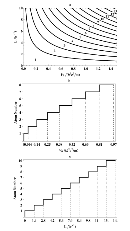
Figure 4: Map of number states and the ionization thresholds for sodium atoms in 1D optical trap in adiabatic limit. Transverse trapping frequency $\omega_{\perp}=2\pi\times 150$ kHz and zero magnetic field are assumed. Note that $c^{-1}$ and $\hbar^{2}c^{2}/m$ are used to make the axes dimensionless. a. Contour plot of number states as function of trap depth and size; b. and c. cross-sectional cut views at the indicated trap size ($5\mu$m) and depth ($4$nK) (solid lines) of a. The ticks on horizontal axes give the calculated ionization thresholds.

Now that we have a clear upper limit, the trap capacity, on the number state that may be present for a given trap and other physical parameters. It remains questionable whether or not the trap capacity can be reached. The adiabatic laser culling technique developed in Ref. Dudarev:2007 and the simulations in Tonks-Girardeau region made in Ref. ACampo:2008-2009 seem to suggest that it is possible to reach the trap capacity with the ultra-cold technique developed in Ref. Chuu:2005 ; Meyrath:2005 .

The starting point is a almost-pure Bose Einstein condensate (BEC) that is optically trapped. Ignore excitation effects for now, it is useful to view the process from the angle of quantum optics and regard the state of the BEC as a coherent state Andrews:1997 . A coherent state is essentially a superposition of Fock states with a Poisson-distribution in the boson numbers. As we adiabatically change experimental parameters from partitions with higher trap capacity to lower capacity targeting some number state, the Bethe ansatz solution puts a tighter and tighter restriction on the maximum number state. The system state thus undergoes two changes side by side: 1, more and more high-energy atoms are forced out; 2, more and more high-number Fock states are quantum mechanically ‘projected’ out of the system state (resulting in the so-called squeezed state). Each of these two changes has its distinctive effect on the system state: the first leads to smaller and smaller average particle number $\overline{N}=\left\langle N\right\rangle$ whereas the second leads to a reduction in the number uncertainty $\sigma^{2}=\left\langle N^{2}-\overline{N}^{2}\right\rangle$. Under optimal experimental conditions, the process continues until at some point, while the average number $\left\langle N\right\rangle>0$, the number uncertainty $\sigma\approx 0$. A rigorous simulation of this would require calculating the value $\frac{\sigma}{\overline{N}}$ as a function of time in a dynamic process and is certainly beyond the scope of this article. In Fig. 4, we show trap capacities and ionization thresholds as functions of trap depth and size. The interaction strength is implicit in the unit we adopted.

There are several ways to tune the physical parameters to achieve the above goals. In previous references Dudarev:2007 ; ACampo:2008-2009 , only culling (changing trap depth), squeezing (changing trap size), or some combinations of the two are discussed. In certain circumstances, we propose that atom-atom interaction strength $c$ be possibly tuned to supplement the production of number states. In view of the intrinsic limitations in tuning the trap parameters, it’s possible that tuning of interaction strengths could play a key role in number state experiments.

The path to a number state becomes clear now. By tuning the physical parameters of the 1D optical trap adiabatically, we force the ultracold atom sample through a series of quantum collapses until it eventually reaches the desired Fock state with some acceptable fidelity. Ideally, the course connecting the starting point and a targeted Fock state consists of a series of states (the Bethe ansatz states) with well-defined particle number. But in reality, there are always some elementary excitations, which is defined as any deviation from the ideal adiabatic course. Possible elementary excitations include occupations of excited Bethe ansatz state (of the same particle number), earlier ionizations (loss of particles before reaching the Bethe ansatz ionization threshold), and simultaneous ionizations of more than one particles.

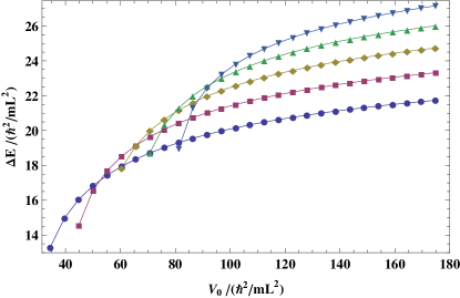
Figure 5: (color online) Excitation energy gaps between ground and first-excited states as function of trap depth for 2 (circle), 3 (square), 4 (diamond), 5 (upright triangle), and 6 (invert triangle) sodium atoms. Trap size is $5\mbox{ }\mu$m.

We now analyze the effects of excitations. Abrupt changes in the trapping potential tend to introduce extra terms into the system density matrix. As the system gets near an ionization threshold, the system becomes particularly delicate, since the particle with the highest energy can tunnel further away from the center of the trap and thus external disturbance has bigger exciting effect on the system. Moreover, immediately after the ionization threshold is passed, the system density matrix is subject to various excitations due to wavefunction collapses. These excitations are crucial to the fidelity of Fock state production, since they cause significant reversion in the number uncertainty of the final state. A characteristic measurement of tendency of excitation is the energy gap, $\Delta$, which is define as the difference between total energies of ground and first-excited Bethe ansatz states (if both exist). According to our calculation, they are on the order of a few $k_{B}\times 10$nK (see Fig. 5). $\Delta$ puts restrictions in two-fold. Firstly, the temperature must be maintained lower than a few $10$nK, otherwise, fidelity could be endangered due to thermal excitation. Furthermore, the energy gap puts a requirement on the adiabaticity condition adiab:theorem : the culling speed must be much smaller than $\frac{\Delta^{2}}{\hbar}$ to maintain a relatively high fidelity. To give a sense of number, we consider the culling of trapping potential from the ionization threshold of 3 particles down to that of 2 particles at trap size of $5\mu$m and transverse trapping frequency $\omega_{\perp}=2\pi\times 150$kHz. According to our calculation, the minimum time required to complete this portion of the culling should be no less than $0.3$ms to be considered as adiabatic.

V conclusion

In conclusion, we calculated the conditions for number states of ultracold atoms in 1D optical trap with the Bethe ansatz approach. We charted ionization thresholds in the parameter space. We also discussed the quantum mechanical processes in producing number states in the ideal case and the effect of excitations.

Appendix A Valid Bethe ansatz solutions

First of all, we need a change of unit to make the dependence of secular equation on interaction strength explicit. (See Section I for the previous choice of unit.) To that end, we choose the trap length $L$ as the length unit, $\hbar^{2}/mL^{2}$ as the energy unit. Then the secular equation Eq.(17) is transformed to

$$-k_{j}L=\pi I_{j}+2\sin^{-1}{\left(\frac{k_{j}}{V_{0}}\right)}+$$ (18)

$$\sum_{l\neq j}{\left[\tan^{-1}{\left(\frac{k_{j}+k_{l}}{c}\right)}+\tan^{-1}{\left(\frac{k_{j}-k_{l}}{c}\right)}\right]},$$

Now Eq.(18) depends both on the set of integers $I$ and the interaction strength $c$. For the mere purpose of solving Eq.17, any set of integers $I$ may be used. Note that the choice of integers is discrete and is usually enumerable while that of the interaction strength $c$ is continuous and non-enumerable. Based on this fact, we claim that if a given set of integers lead to valid solution at some interaction strength, it does so at any interaction strength. Particularly, the solution in the weak interaction region should approach that of the non-interacting case as $c\to 0$. Solution of the latter is a well-taught exercise in many quantum mechanics textbooks.

Thus, a ‘promising solution’ to Eq.(18) should converge onto that of the $c=0$ case and we can use the known solutions to reject spurious ‘solutions’ for the interacting cases. With a few examples of $N$ and upper limits $M$, we exhaust all the combinadics of $N$ numbers from the range $[0,M]$ and solve Eq.(18) with each combination. Our experiments show that in the limit $c\to 0$, a solution approaches that of $c=0$ if and only if the set $I$ consists of positive and mutually distinct integers. Furthermore, we also find that the wave numbers in the solution are mutually distinct if and only if the integers in the set $I$ are mutually distinct.

Appendix B Order of Bethe ansatz states

With the valid solutions found in Appendix A, it still left to determine which one is the ground state and which is the first excited state, and so on. In a similar manner as in Appendix A, we will argue based on intuition that for any given $N$, the set $I=\{1,2,\cdots,N\}$ leads to the ground state and the set $I=\{1,2,\cdots,N-1,N+1\}$ to the first excited state.

Our clue comes from the strong interaction limit. As is well known, in the strongly interacting limit the particles behave as fermions Girardeau:1960 . Thus the ground state of our system must be like that of a degenerate fermion system. Our numerical calculations show that solving Eq.(18) with the set $I=\{1,2,\cdots,N\}$ leads to a solution with energy that approaches that of the ground state of the degenerate fermion system in the limit $c\to\infty$. Furthermore, the solution obtained with the set $I=\{1,2,\cdots,N-1,N+1\}$ approaches that of the first-excited state of the same system in the same limit. We thus established what are ground state and first excited state for our system in general. However, there is little we could say beyond that. Within limit of calculation error, our experiment is not conclusive about which is the second excited states. It might be $1,2,\cdots,N-1,N+2$, $1,2,\cdots,N-2,N,N+1$, or still other, depending on $N$ and the trap parameters. In general the order in the energy level of a Bethe ansatz state depends on both the highest quantum number and the total of these quantum numbers. For complete ordering, one need something as what Hund’s Rule is in atomic physics. For our paper, it suffices to know just the ground state and first excited state.

References

- (1) D. Jaksch, H.-J. Briegel, J.I. Cirac, C.W. Gardiner, and P. Zoller, Phys. Rev. Lett. 82, 1975 (1999).
- (2) A.M. Dudarev, R.B. Diener, B. Wu, M.G. Raizen, and Q. Niu, Phys. Rev. Lett. 91, 010402 (2003).
- (3) E. Andersson and S.M. Barnett, Phys. Rev. A 62, 052311 (2000).
- (4) T.P. Meyrath, et al., Phys. Rev. A 71, 041604 (2005); T.P. Meyrath, et al., Opt. Express 13, 2843 (2005).
- (5) C.-S. Chuu, F. Schreck, T.P. Meyrath, J.L Hanssen, G.N. Price, and M.G. Raizen, Phys. Rev. Lett. 95, 206403 (2005).
- (6) A.M.Dudarev, M.G. Raizen, and Q. Niu, Phys. Rev. Lett. 98, 063001 (2007).
- (7) A. del Campo and J.G. Muga., Phys. Rev. A 78, 023412 (2008); M. Pons, A. del Campo, J.G. Muga, and M.G. Raizen, Phys. Rev. A 79, 033629 (2009).
- (8) Inouye, S. et al. Nature 392, 151 (1998); Courteille, Ph., Freeland, R. S., Heinzen, D. J., van Abeelen, F. A. and Verhaar, B. J., Phys. Rev. Lett. 81, 69 (1998).
- (9) Girardeau, M., J. Math. Phys. 1, 516 (1960).
- (10) There are other technical reasons in tuning the interaction strength. To facilitate efficient loading of Bose Einstein condensate into the optical box, the transverse trapping frequency is often relaxed in the beginning and tightened up toward the end to promote atom-atom interaction. This process often gets involved with that of the number-state production. Therefore, we need to study the connections across various interaction regimes.
- (11) H.A. Bethe, Zeitschrift für Physik 71, 205 (1931), see also the English translation in ”Selected works of Hans A. Bethe: with commentary”, ISBN 9810228767, World Scientific, 1997.
- (12) R.Orbach, Phys. Rev. 112, 309 (1958).
- (13) L.R. Walker, Phys. Rev. 116, 1089 (1959).
- (14) E. Lieb, T. Schultz and D. Mattis, Ann. Phys. (N.Y.) 16, 407 (1961).
- (15) E.H. Lieb and W. Liniger, Phys. Rev. 130, 1605 (1963); E.H. Lieb, ibid. 130, 1616 (1963).
- (16) J.B. McGuire, J. Math. Phys. 5, 622 (1964).
- (17) C.N. Yang, Phys. Rev. Lett. 19, 1312 (1967).
- (18) B. Sutherland, Phys. Rev. Lett. 20, 98 (1968); J. Math. Phys. 21, 1770 (1980).
- (19) Y. Hao, Y. Zhang, J.Q. Liang, S. Chen, Phys. Rev. A 063617 (2006).
- (20) M. Gaudin, Phys. Rev. A 24, 55 (1967).
- (21) Y.Q. Li, Phys. Rev. A 52, 65 (1995).
- (22) M. Olshanii, Phys. Rev. Lett. 81, 938 (1998).
- (23) M.R. Andrews, C.G. Townsend, H.-J. Miesner, D.S. Durfee, D.M. Kurn, and W. Ketterle, Science, 275, 637 (1997).
- (24) Y. Aharonov and J. Anandan, Phys. Rev. Lett. 58, 1593 (1987).