Bolometric Light Curves for 33 Type II-Plateau Supernovae

Abstract

Using data of three well-observed type-II plateau supernovae (SNe II-P), SNe 1987A, 1999em and 2003hn; and two atmosphere models by Eastman et al. (1996) and Dessart $\&$ Hillier (2005b) we derive calibrations for bolometric corrections and effective temperature from BVI photometry. The typical scatter of the bolometric correction is 0.11 mag. With these results we obtain bolometric light curves and effective temperature evolution for a sample of 33 SNe II-P. The SN sample shows a range of 1 dex in plateau luminosity and plateau durations from 75 to 120 days. Comparing the shape of the transition between the plateau and the radioactive tail, we find that the size of the drop is in the range of 0.8 to 1.12 dex.

1 INTRODUCTION

Nowadays we know that the type II plateau supernovae, the most common type of supernovae (SNe) in nature (Mannucci et al., 2005; Cappellaro et al., 2005; Smartt et al., 2009), are part of a larger group known as “core-collapse supernovae” (CCSNe) —which includes type Ib, type Ic, and other subclasses of type II SNe (Filippenko, 1997)— sharing, in general terms, the same explosion mechanism (Burrows, 2000; Gal-Yam et al., 2007). Stars which are born with masses above 8 M_⊙ are thought to end their lives as CCSNe (Heger et al., 2003; Eldridge & Tout, 2004). The observational characteristics of these events strongly depend on the final stage of the progenitor object and on the properties of the circumstellar medium at the time of explosion. In the case of type II plateau supernovae (SNe II-P) it is believed that the progenitors are red supergiants with thick hydrogen envelopes (generally several solar masses) (Grassberg et al., 1971; Falk & Arnett, 1977; Litvinova & Nadezhin, 1983; Smartt et al., 2004). It is this particular feature and the fact that the star explodes in a very low-density environment (Baron et al., 2000; Chevalier et al., 2006) which are responsible for the type II classification (H lines in the spectrum) and also for the plateau typing (plateau-shaped light curve).

The study of SNe II-P is critically important for understanding the range of progenitor masses, radii and energies which produce these objects. One way to estimate such parameters is by comparing observations (light curves, colors, spectra) with hydrodynamical models. Some of the classical theoretical studies are those by Litvinova & Nadezhin (1983) and Litvinova & Nadezhin (1985). Attempts to compare these models with observations have been addressed by Hamuy (2003) and Nadyozhin (2003). However, these studies have not been satistactory owing to 1) the lack of good-quality data, 2) the usage of simplified relations between ill-defined and hard-to-measure photometric and spectroscopic parameters, and 3) the fact that some of the models are based on simplified physical assumptions.

In order to improve this situation, we have 1) enlarged the database of spectra and light curves for 33 SNe II-P, and 2) developed our own hydrodynamical models using better physics. Since our code produces bolometric light curves and effective temperatures, it proves necessary to calculate these quantities from the observed photometry. Our final goal is to do this comparison for the 33 SNe, but only three of them (SN 1987A, SN 1999em, and SN 2003hn) were observed over a sufficiently broad wavelength range to allow the calculation of bolometric fluxes. The purpose of this paper is to 1) use the data for these three well-observed objects and explore the feasibility to derive a bolometric correction that could be applied for the remaining SNe with optical observations alone, and 2) derive a calibration for effective temperature from optical colors.

Here we focus only on SNe II-P since these objects possess extended, spherically symmetric hydrogen envelopes which smooth out possible inhomogeneities arising from differences in the explosions themselves (Chevalier & Soker, 1989; Leonard & Filippenko, 2001). Therefore, at least during the optically thick plateau phase, we expect a photosphere radiating as a “dilute” blackbody whose properties are mainly driven by the photospheric temperature (Eastman et al., 1996; Dessart & Hillier, 2005a). As the SN expands the temperature drops monotically, so we expect a regular spectroscopic evolution for this class of objects, and a well-behaved bolometric correction with color during the plateau phase. The inhomogeneities are expected to become more noticeable by the end of the plateau, at which point the hydrogen envelope is almost completely recombined, the photosphere lies near the center of the object, and the inner layers becomes visible.

Usually the approach used to calculate bolometric light curves consists in integrating the flux observed in all available photometric bands and making some assumption about the missing flux based on spectroscopic observations or models (Elmhamdi et al., 2003; Folatelli et al., 2006). Here we propose a quantitative method to estimate the missing flux in the ultraviolet and infrared ranges using data from the three well-observed SNe, and two sets of atmosphere models. The derived bolometric corrections correlate so well with optical colors that this calibration can be used to calculate bolometric light curves for many other SNe II-P having $BVI$ photometry alone, opening thus the possibility for a statistical analysis of the physical properties of this type of objects.

We begin in § 2 by describing the observational and theorical material used and the procedure followed to calculate bolometric luminosities. In § 3 we derive calibrations for the bolometric correction and effective temperature as a function of colors. Then in § 4 we apply these calibrations to obtain bolometric luminosities and effective temperatures for the sample of 33 SNe II-P presented by Hamuy et al. (2009). Finally in § 5 we outline our main results and conclusions of this paper. In an upcoming paper (Bersten et al., 2009) we will present theoretical light curves from our hydrodynamical models in order to derive physical parameters for this set of SNe.

2 Bolometric Flux for Calibrating Supernovae and Atmosphere Models

In this section, we describe how we calculate bolometric fluxes for the three SNe II-P which possess UV, optical and IR photometry, namely, SN 1987A, SN 1999em and SN 2003hn, and the two sets of atmosphere models available in the literature (Eastman et al., 1996; Dessart & Hillier, 2005a) (E96 and D05 hereafter, respectively). This is our first step in order to examine if a bolometric correction can be derived from optical photometry alone. From now on, we will refer to the SN evolution in terms of time or color indistinctly. This is well justified during the plateau phase in which the SN atmosphere expands, cools and monotically turns reddder.

2.1 Observational and Theoretical Data

In order to examine if a bolometric correction can be derived from optical colors, we made use of the three SNe II that possess the best wavelength and temporal coverage. Two of these are genuine SNe II-P, SN 1999em and SN 2003hn, and the third is the famous SN 1987A which, except for its peculiar light curve, shares most of the spectroscopic properties of SNe II-P. Most of the data of these three SNe was obtained at Cerro Tololo Inter-American Observatory (CTIO), Las Campanas Observatory (LCO), and the European Southern Observatory (ESO) at La Silla. For more details about the data reduction and instruments used see Hamuy & Suntzeff (1990) and Bouchet et al. (1989) for SN 1987A, Hamuy et al. (2009) for SN 1999em, and Krisciunas et al. (2009) for SN 2003hn. The photometric bands used in this analysis were $UBVRIZJHK$ for SN 1999em and SN 2003hn, and $UBVRIZJHKLM$ for SN 1987A.

We adopted Cepheid distances for SN 1987A and SN 1999em with corresponding values of 50 kpc (Freedman et al., 2001) and 11.7 Mpc (Leonard et al., 2003). For SN 2003hn we used a distance of 16.8 Mpc, as derived by Olivares et al. 2008 using the Standardized Candle Method. We corrected the photometry for Galactic and host-galaxy extinction. We performed such corrections using Galactic visual absorptions of A${}_{V}^{GAL}$=0.249 for SN 1987A, A${}_{V}^{GAL}$=0.13 for SN 1999em, and A${}_{V}^{GAL}$=0.043 for SN 2003hn (Schlegel et al., 1998), assuming a standard reddening law with R_V= 3.1 as given by Cardelli et al. (1989). The values used for host-galaxy absorption were, A${}_{V}^{host}$=0.216 for SN 1987A, A${}_{V}^{host}$=0.18 for SN 1999em (Hamuy, 2001) and A${}_{V}^{host}$=0.56 for SN 2003hn (Dessart, 2008), again assuming R_V= 3.1.

We also used in this analysis spectral energy distributions (SEDs) from two sets of SN atmosphere models (E96 and D05). These models depend on several parameters such as, luminosity, density structure, velocity and composition. For more details on the input parameters of such models the reader is referred to Eastman et al. (1996) and Dessart & Hillier (2005a). We used a total of 61 model spectra from E96, and 107 from D05. We discarded 31 spectra from D05 which did not have enough UV coverage.

2.2 Bolometric Luminosity Calculations

By definition, the bolometric luminosity is the integral of the flux over all frequencies. This integration can be done in a straight-forward way for the spectral models of E96 and D05 summing the flux over wavelength. With the purpose to estimate bolometric corrections and colors for the models we computed $BVI$ synthetic magnitudes using the filter transmission functions and zero points given by Hamuy (2001).

For the three well-observed SNe the calculation of bolometric luminosities was performed from reddening-corrected broadband magnitudes using the values mentioned in section  2.1. K-corrections were negleected due to the small redshifts involved. We began by computing a quasi-bolometric light curve using all the available broadband data. The magnitudes were converted to monochromatic fluxes at the specific effective wavelength of each filter using the transmission functions and zero points of the photometric system (Hamuy, 2001). At epochs when a certain filter observation was not available, we interpolated its magnitude in time using the closest points. The total “quasi-bolometric” flux, $F_{qbol}$ was computed using trapezium integration.

To estimate the missing flux in the UV and IR, $F_{UV}$ and $F_{IR}$, we fitted at each epoch a blackbody (BB) function to the monochromatic fluxes. At early epochs the BB model provided very good fits to the fluxes in all bands. As the photosphere became cooler the $U$-band flux started to depart from the BB model in which cases we excluded this point from the fit. At later epochs, subsequently the $B$-band and $V$-band data points showed the same behavior, departing from the BB model. The reason for this is related to the strong line blanketing that develops with time in that part of the spectrum.

On the IR side the flux was extrapolated to $\lambda=\infty$ using the BB fits described above. The integral of that function between the longest observed effective wavelength and $\lambda=\infty$ was adopted as the IR correction (F_IR). This correction increased with time but it always remained below 7$\%$ for the three SNe.

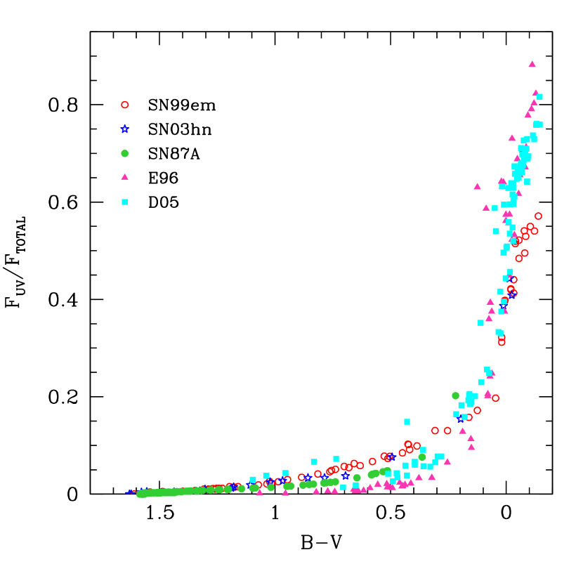
Figure 1: UV contribution to the total flux as a function of $(B-V)$ for the SN 1987A, SN 1999em and SN 2003hn and for the models of E96 and D05. At early times, when $(B-V)\lesssim 0.2$, the UV flux represents a significant fraction of the total flux, implying larger uncertainties in the UV correction.

On the UV side, we extrapolated from the effective wavelength of the $U$ band to $\lambda$=0 using the BB fit on all epochs except when the $U$-band flux fell below the BB model. In these cases, we extrapolated the $U$-band flux using a straight line to zero flux at 2000 Å. Our choice of $\lambda$= 2000 Å as the wavelength where the flux goes to zero was based on the behavior of the atmospheric models for which the flux blueward of 2000 Å is negligible in comparison with the total flux. The integrated flux under the Plank function (or straight line) between the effective wavelength of the $U$ filter and $\lambda$=0 (or $\lambda$=2000 Å) was taken as the UV correction (F_UV). The size of this correction relative to the total flux for the three SNe and the two sets of atmospheric models is shown in Figure  1 as a function of $(B-V)$. The first thing to note is the overall good agreement in F_UV between the observed SNe and the atmopshere models. Second, it is evident that the UV correction is very important at early epochs and becomes nearly irrelevant at the latest epochs. Thirdly, note that in the very blue end, where the UV corrections are of order 50-80%, there is some disagreement between the atmosphere models and SN 1999em. The spectral models suggest larger UV corrections and, as argued below, they are more thrustworthy at these early epochs than the extrapolation of the broadband magnitudes. To prove this point, we calculated F_UV for the models using the same technique that we employed for SN 1999em, i.e. by computing synthetic magnitudes for all passbands, converting them to monochromatic fluxes, and fitting a BB to the resulting points (instead of the direct integration of the SED). In this case the UV correction proved closer to the UV correction derived from SN 1999em. We conclude that the UV extrapolation using the BB fits to the broadband magnitudes at very early epochs underestimates somewhat F_UV, so we ended up using only the atmosphere models at such epochs. At later times ($B-V$$>-0.04$), where the differences between data and theory become negligible, we adopted both the models and the observed data.

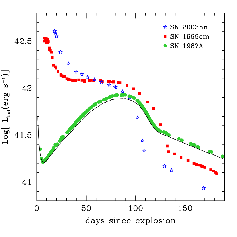
Figure 2: Bolometric luminosity of SN 1987A, SN 1999em and SN 2003hn computed from the integration of broadband optical and near-infrared data plus UV and IR contributions as explained in section 2.2. For comparison we included the bolometric luminosity of SN 1987A obtained by Suntzeff & Bouchet (1990)(solid line).

The sum F_qbol+F_UV+F_IR yielded the bolometic flux F_bol. Then we transformed flux into luminosity using the distances given in section 2.1. The resulting bolometric luminosities for SN 1987A, SN 1999em and SN 2003hn are shown in Figure  2. As a comparison, the solid line shows the bolometric luminosity of the SN 1987A obtained by Suntzeff & Bouchet (1990). We found a very good qualitative agreement between both bolometric light curves for SN 1987A. There is a systematic difference which remains smaller than 0.04 dex at all times between both calculations. Such differences are consistent with the uncertainties estimated for the use of different datasets and different integration and interpolation scheme (Suntzeff & Bouchet, 1990).

As it can be seen in Figure 2, the morphologies of the bolometric light curves for the three SNe are differents, specially that of SN 1987A which shows a broad maximum, not observed in the classical SN II-P, and a less luminous light curve (up to the transition to the radioactive tail). It is a well known fact that SN 1987A showed a peculiar light curve and this was because its progenitor was a compact blue supergiant that lead to a dim initial plateau and to a light curve promptly powered by radioactivity (Woosley, 1988; Shigeyama & Nomoto, 1990) . However, the three SNe showed a similar initial phase where the supernova rapidly faded and cooled until the outermost parts of the ejecta reached the temperature of hydrogen recombination (adiabatic cooling phase). A second phase can be distinguished for SN 1999em and SN 2003hn which corresponds to the plateau where the brightness of the supernovae remained nearly constant while hydrogen is recombining (Grassberg et al., 1971). The duration and the slope of the light curve during this phase were different for each supernova. This is related to the properties of the progenitor object, mainly to the mass and radius of the hydrogen envelope. The shape of the light curve for the SN 1987A during this phase was very different as mentioned above. It showed a broad maximum characterize by a slow rise of $\sim$ 90 days followed by a more rapid decline for about 30 days. Finally, we can distinguish a third phase the radioactive tail which has a similar shape for the three SNe. Here, the luminosity has a lineal behavior and it is dominated by radioactive decay of ⁵⁶Co. The luminosity in this part of the light curve is a direct indicator of the mass of ⁵⁶Ni synthesized in the explosion (Woosley et al., 1989), in the sense of that more luminosity implies more ⁵⁶Ni mass. We deduce from this that SN 1987A produced more ⁵⁶Ni than the other two SNe.

3 Calibrations

3.1 Bolometric corrections versus Color

There are many SNe that lack IR and UV observations for which it is not possible to calculate the bolometric luminosity using the method described in the previous section. For these cases it is necessary to know the bolometric correction required to convert a $V$-band magnitude into a bolometric flux, i.e.,

$$BC=m_{bol}-[V-A_{V}],$$ (1)

where $A_{V}$ is the total visual extinction and $m_{bol}$ is the bolometric magnitude in the Vega system. Note that, since BC is defined as a magnitude difference, it is independent of the distance assumed for each object.

We calculated BC at all epochs for each of the calibrating SNe and for all of the SN models using the bolometric luminosities computed in section 2.2. The bolometric fluxes were converted into Vega magnitudes in the following manner,

$$m_{bol}=-2.5\,\,log_{10}\,\,F_{bol}\,+11.64,$$ (2)

where the zeropoint is obtained by integrating the SED of Vega given by Hamuy(2001) and forcing the resulting magnitude to vanish, i.e., m_bol(Vega)= 0.

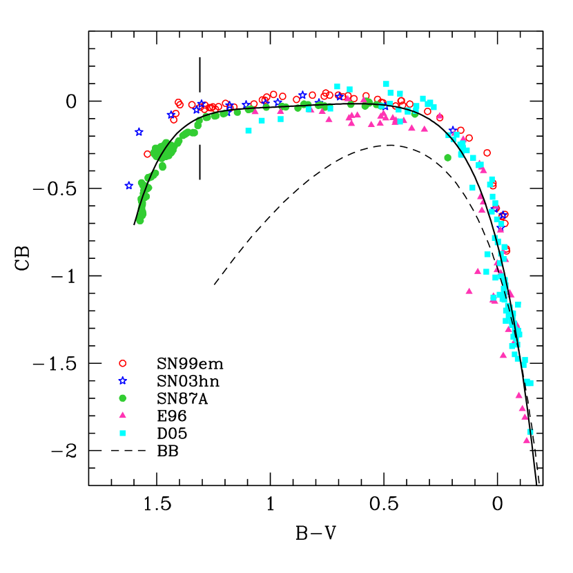
Figure 3: Bolometric corrections versus $(B-V)$ for SN 1999em (open circles), SN 2003hn (stars), SN 1987A (filled circles) and the models of E96 (triangles) and D05 (squares). The vertical lines indicate the color end at the the plateau phase. The solid line shows a polynomial fits to the points. The dashed curve correspond to the bolometric corrections of a blackbody spectrum.

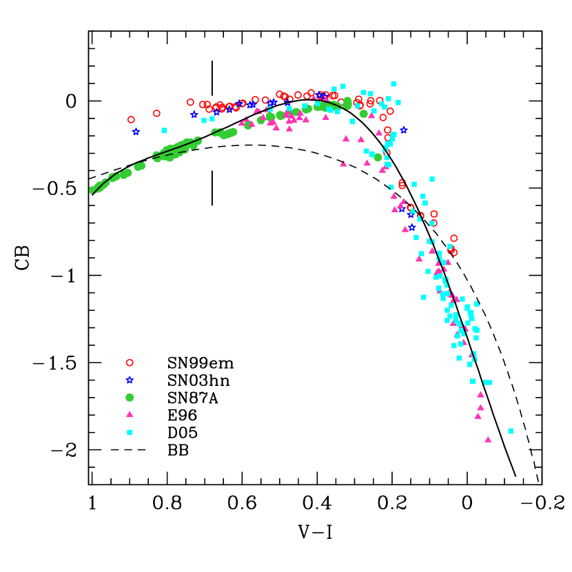
Figure 4: Bolometric corrections versus $(V-I)$ for SN 1999em (open circles), SN 2003hn (stars), SN 1987A (filled circles) and the models of E96 (triangles) and D05 (squares). The vertical lines indicate the color end at the the plateau phase. The solid line shows a polynomial fits to the points. The dashed curve correspond to the bolometric corrections of a blackbody spectrum.

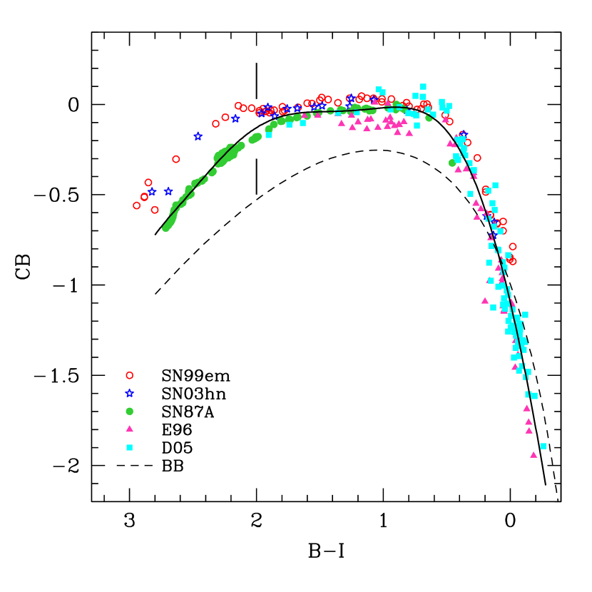
Figure 5: Bolometric corrections versus $(B-I)$ for SN 1999em (open circles), SN 2003hn (stars), SN 1987A (filled circles) and the models of E96 (triangles) and D05 (squares). The vertical lines indicate the color end at the the plateau phase. The solid line shows a polynomial fits to the points. The dashed curve correspond to the bolometric corrections of a blackbody spectrum.

We analyzed the dependence of the BC on color, using $(B-V)$, $(V-I)$ and $(B-I)$. The main reason why we did not try colors involving the $R$ band is because our sample (Hamuy et al., 2009) has few SNe with $R$-band observations. Figures 3, 4 and 5 show the resulting corrections as a function of the mentioned colors (corrected for dust) for SN 1987A, SN 1999em, SN 2003hn, and the models of E96 and D05. In each of these plots the vertical bar indicates the approximate color corresponding to the end of the plateau (see section 4 for a precise definition of plateau phase). To the red of this mark are shown the BC corresponding to the transition between the plateau and the radioactive tail for the three SNe (no atmosphere models cover this phase). We do not include any of the nebular data in these diagrams, since the BB fits are not appropriate to extrapolate UV or IR fluxes at these epochs.

These plots reveal a remarkable correlation between BC and intrinsic color, both for the objects and the models. It is very satisfactory that, even though SN 1987A has a very different light curve compared with normal SNe II-P, it matches quite well the behavior of the other two SNe and the models. At very early times the BCs are quite large owing to the relatively larger flux contribution of the UV. During most of the plateau the BC remains very small around a value of zero, which implies that the $V$ magnitude provides a very close proxy for the bolometric magnitude. During the transition from the plateau to the radioactive tail (redward from the vertical bar) the BC starts to depart from zero due to the larger flux contribution in the IR. At these phase SN 1987A shows some discrepancies, at the level of $\sim$0.1-0.2 mag, with respect to the other two SNe. Since the bolometric fluxes for SN 1987A comprise two more IR bands, $L$ and $M$, we examined the possibility that these discrepancies could be due to this fact. For this, we excluded the $L$ and $M$ bands for SN 1987A and recomputed the bolometric flux in the same manner as for the other two SNe, i.e, by calculating $F_{IR}$ as the extrapolation of a BB fit to $U-K$ photometry. This exercise showed that, while the BC corrections over the plateau phase do not change in any significant way (lending support to the $F_{IR}$ derived from BB fits), by the end of the plateau and at later times the new BCs increase and get closer to the other two SNe. The conclusion is that the differences observed during the transition are due to an inaccurate estimate of $F_{IR}$ from the BB fits restricted to $U-K$ photometry. Adding $L$ and $M$ photometry at these late epochs do help and provides a more accurate estimate of $F_{IR}$. Therefore, during the transition we decided to exclude the BCs derived from SN 1999em and 2003hn.

A good representation of the correlation between BC and colors can be obtained with polynomial fits of the form,

$$BC(color)=\sum_{i=0}^{n}a_{i}\,(color)^{i},$$ (3)

where the order $n$ varies for each color. Table  1 lists the coefficients obtained for the fit of each color, their range of validity and the number of data points used. The fits have dispersions (rms) of 0.11 mag for ($B-V$), 0.11 mag for ($V-I$) and 0.09 mag for ($B-I$) in the whole range (plateau plus transition to the radioactive tail).

The corresponding polynomials fits are also shown with solid lines in Figure 3, 4 and 5. As a comparison, the dashed line in these Figures show the BC derived for a blackbody. The blackbody models represent well the data at early times (bluest colors), but evidently differ from the atmosphere models and the observed SNe at later epochs.

As argued in section  2.2, we have good reasons to trust more the atmopshere models than the early data of SN 1999em, so we decided to exclude the latter from our fits. Therefore, our calibration should be considered more uncertain here. A further complication at early phases is the steep dependence of the BC on color. This means that a slight error in the measurement of the color, such as that due to a poor extinction determination, could cause a significant error in the determination of the BC. This problem is less pronounced if we use $(V-I)$ to estimate BC at these epochs. We also tested if a bolometric correction with respect to the $R$ band instead of $V$ would improve the situation, but we did not find any improvement.

Using the coefficients given in Table  1, it is possible to derive a bolometric luminosity for any SN II-P using only two (or three in the case of the $(B-I)$ color) optical filters. If one knows the extinction and the distance to the object the bolometric luminosity can be computed as,

$$\log L[\mathrm{erg\,~{}s}^{-1}]=-0.4\,\,[BC(color)+V-A_{total}(V)-11.64]+\log(4\,\pi D^{2}),$$ (4)

where $D$ is the distance in cm to the SN and $A_{total}(V)$ is the total, host plus Galactic, visual absorption. Note that combining this equation with equations (1) and (2), the luminosity becomes independent of the arbitrary zero points chosen for the Vega magnitude scale, and it only depends on the observed flux density, color, extinction and distance.

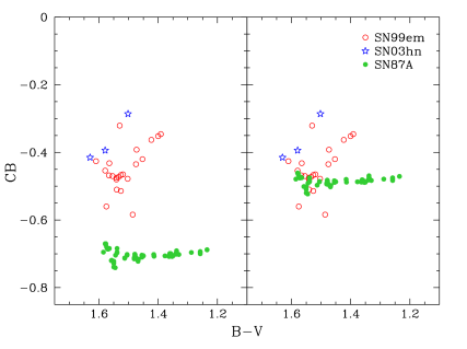
Figure 6: (Left) Bolometric corrections obtained during the radioactive tail phase versus $(B-V)$, as derived using $U$ thru $M$ photometry for SN 1987A (filled circles), and $U$ thru $K$ photometry for SN 1999em (open circles) and SN 2003hn (stars). (Right) Same as before, but excluding the $L$ and $M$ bands for SN 1987A.

The calibrations of BC versus colors shown above are only valid during the optically thick phases since they involve BB fits to the photometry. In the nebular phase, we calculated BCs for the three SNe using the integrated flux between the observed bands (i.e. $U-K$ for SN 1999em and SN 2003hn, and $U-M$ for SN 1987A). We did not attempt to add any flux beyond these limits since we did not have any physical model to extrapolate. As shown in the left panel of Figure 6 the BC for SN 1987A is almost independent of color, with a value of $-0.70$ mag and a scatter of only 0.015 mag. The other two SNe yield BCs 0.2–0.3 mag higher, with a slight dependence on color. We investigated whether this differences could be due to the inclusion of the two additional bands for SN 1987A: we removed the $L$ and $M$ bands from the BC and, not surprisingly, the agreement proved very good (Right panel of Figure 6). We conclude that the $L$ and $M$ contributions to the bolometric flux is not negligible at the nebular phase. Hence, we take the value of $-0.70$ derived from SN 1987A as the best estimate of the BC at the onset of the nebular phase.

We conclude this section with the claim that we have implemented a robust method to estimate BCs for SNe II-P which allows one to derive bolometric luminosities. If we trust the late behavior of SN 1987A as being representative of SNe II-P in general, our analysis implies an overall accuracy of 0.05 dex in BCs. Clearly, it would be interesting to check this result using L and M photometric data of other SNe II-P, but such data are currently unavailable. Our calibrations have the potential to be applied to many SNe observed over a limited wavelength range.

3.2 Effective Temperature-Color Relation

Along with bolometric luminosity, the effective temperature is a critical parameter in the comparison of observations with hydrodynamical models. Each model spectrum of E96 and D05 has an associated effective temperature (T_eff), defined by the relation $L=4\pi R_{ph}^{2}\sigma T_{eff}^{4}$ where L is the input luminosity of the atmospheric models and $R_{ph}$, the photospheric radius, is an output of the models. We examined the dependence of T_eff on $(B-V)$ and $(V-I)$ colors derived via synthetic photometry from the model spectra, as described in section 2.2. The purpose of this analysis was to provide a calibration between temperature and color which could be used to easily derive estimates of T_eff from observed colors for any SN II-P. Note, however, that T_eff does not have a direct physical meaning for this type of objects. It is simply a convenient contact point between hydrodinamical models and observations.

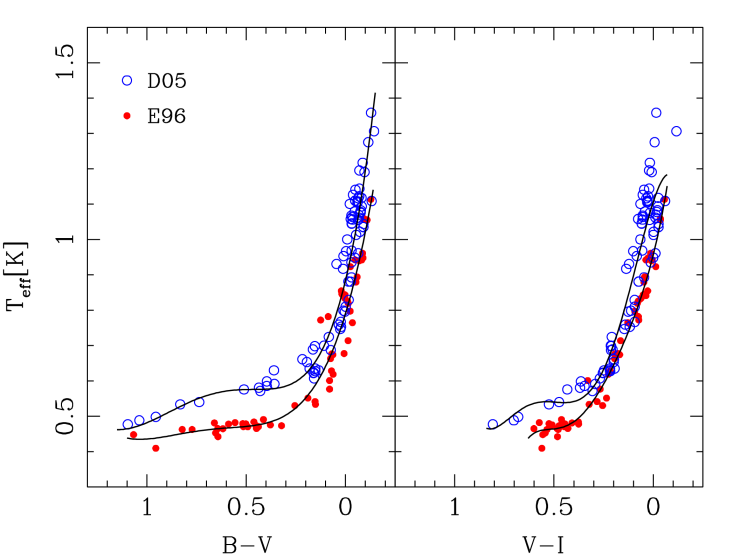
Figure 7: Effective temperature versus $(B-V)$ (left) and $(V-I)$ (right) from the models of E96 (filled circles) and D05 (open circles). The solid lines show polynomial fits for each model set.

Figure 7 shows the effective temperature versus synthetic $(B-V)$ and $(V-I)$ colors for E96 and D05 models. As expected, there is a tight correlation between these quantities for each set of models. At early epochs, when $(B-V)\lesssim 0.2$ and $(V-I)\lesssim 0.3$, both models show consistent values of the effective temperature within their internal dispersion. Later on, however, when the plateau phase is well established, there are systematic differences in the behavior of both sets, with the models of D05 giving larger effective temperatures. Similar differences have been reported in the literature with regard to the dilution factors calculated from both sets of models (Dessart & Hillier, 2005b; Jones et al., 2009), but there has been no clear explanation for the discrepancies. Note that T_eff ( $\propto\sqrt{R_{ph}}$) is an output of the atmosphere model and depends on complicated details of the solution of radiation transport through the envelope, such as non-LTE treatment of the different species and metal line opacities.

In order to represent the correlation between T_eff and colors shown in Figure 7, we fit polynomial functions of the form,

$$T_{eff}(color)[10^{4}K]=\sum_{i=0}^{n}a_{i}\,(color)^{i}.$$ (5)

The fits were done for each set of models separately and they are shown in Figure 7 with solid lines. The coefficients of the fits, ranges of validity for $(B-V)$ and $(V-I)$ colors, and dispersions are given in Table 2. The fits to the E96 models are characterized by a scatter of $\sim$500 K in $(B-V)$ and $\sim$350 K in $(V-I)$. For the D05 models the scatter is $\sim$670 K in $(B-V)$ and $\sim$800 K in $(V-I)$. We do not have any strong argument to rule out either set of models. We therefore keep both results even if they show significant systematic differences. But we notice that the value of T_eff during the recombination phase (where it is nearly constant) appears to be somewhat underestimated (T${}_{eff}\sim 4600$ K) by E96. We recall that these calibrations are only valid until the end of the plateau phase.

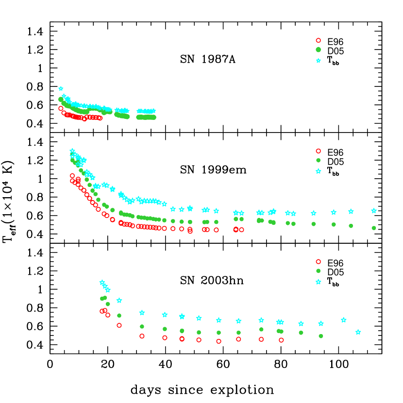
Figure 8: Effective temperatures for SN 1987A (upper panel), SN 1999em (middle panel) and SN 2003hn (bottom panel ) as a function of time since explosion calculated using the polynomial fits given in table 2 for the models of E96 (open circles) and D05 (filled circles). As a comparison we included in these plots the color temperatures obtained from the BB fits described in section 2.2.

In Figure 8 we show how these calibrations work for estimating T_eff for SN 1987A, SN 1999em, and SN 2003hn. As a comparison we included in these plots the color temperatures obtained from the BB fits described in section 2.2. Note that for the three SNe the color temperatures are greater than $T_{eff}$, which is expected for “dilute” atmospheres whose continuum opacity is dominated by electron scattering. As we said before, the usefulness of these fits is that they allow one to obtain T_eff for any SN II-P from their $(B-V)$ or $(V-I)$ colors, and thereby use this quantity to compare with hydrodynamical models. Note that we could equivalently have chosen to calibrate R_ph vs color.

4 Application to SNe II-P Data

We applied our calibrations for bolometric corrections and effective temperatures to a sample of 33 SNe II-P with precise optical photometry. This sample of SNe II-P was observed in the course of four systematic follow-up programs: the Cerro Tololo Supernova Program (1986-2003), the Calán/Tololo Supernova Program (CT; 1990-1993), the Optical and Infrared Supernova Survey (SOIRS; 1999-2000), and the Carnegie Type II Supernova Program (CATS; 2002-2003). Currently, all of the optical data have been reduced and they are in course of publication (Hamuy et al., 2009). Additionally, we included four SNe from the literature: SN 1999gi (Leonard et al., 2002), SN 2004dj (Vinkó et al., 2006), SN 2004et (Sahu et al., 2006), and SN 2005cs (Pastorello et al., 2006; Tsvetkov et al., 2006).

To calculate bolometric light curves for these SNe we only need to apply equation (4). Thus, we need to have (1) $BVI$ photometry, (2) extinction corrections due to our own Galaxy, (3) host-galaxy reddening corrections, and (4) distances.

We obtained Galactic extinction from Schlegel et al. (1998). Host-galaxy extinctions and distances for the present sample were calculated by Olivares et al. (2009) (see their Tables 2.2, 3.1, 4.4) using the Standardized Candle Method. For two objects, SN 2003ef and SN 2005cs, Olivares et al. (2009) did not provide distances. For SN 2003ef we used the EPM distance estimated by Jones et al. (2009) , converted to the distance scale of Olivares et al. (2009) using the conversion coefficients given by the authors. The resulting value was of $48.55$ Mpc. For SN 2005cs we used the distance modulus of $\mu=29.62$ mag given by Pastorello et al 2006, which corresponds to 8.4 Mpc.

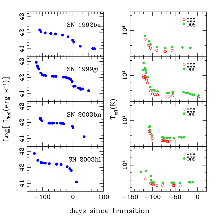
Figure 9: (left) Bolometric luminosity curves for four well-observed objects of our sample: SN 1992ba, SN 1999gi, SN 2003hn, and SN 2003hl. (right) Effective temperatures for the same four SNe. The origin of time in these plots is the middle point between the plateau and the linear tail (Olivares et al., 2009).

We obtained bolometric light curves and effective temperatures for the 33 SNe II-P in the sample and placed them in the same scale of time in order to compare them. Given that we did not have an estimate of the explosion time for the majority of the SNe used in this analysis, we decided to use as origin of time the epoch defined by Olivares 2008 et al., i.e. the middle point of the transition between the plateau and the radioactive tail. Figure 9 shows the bolometric light curves and effective temperatures for a subsample of four objects. Bolometric light curves and effective temperatures for the remaining 29 SNe are provided only in the electronic edition.

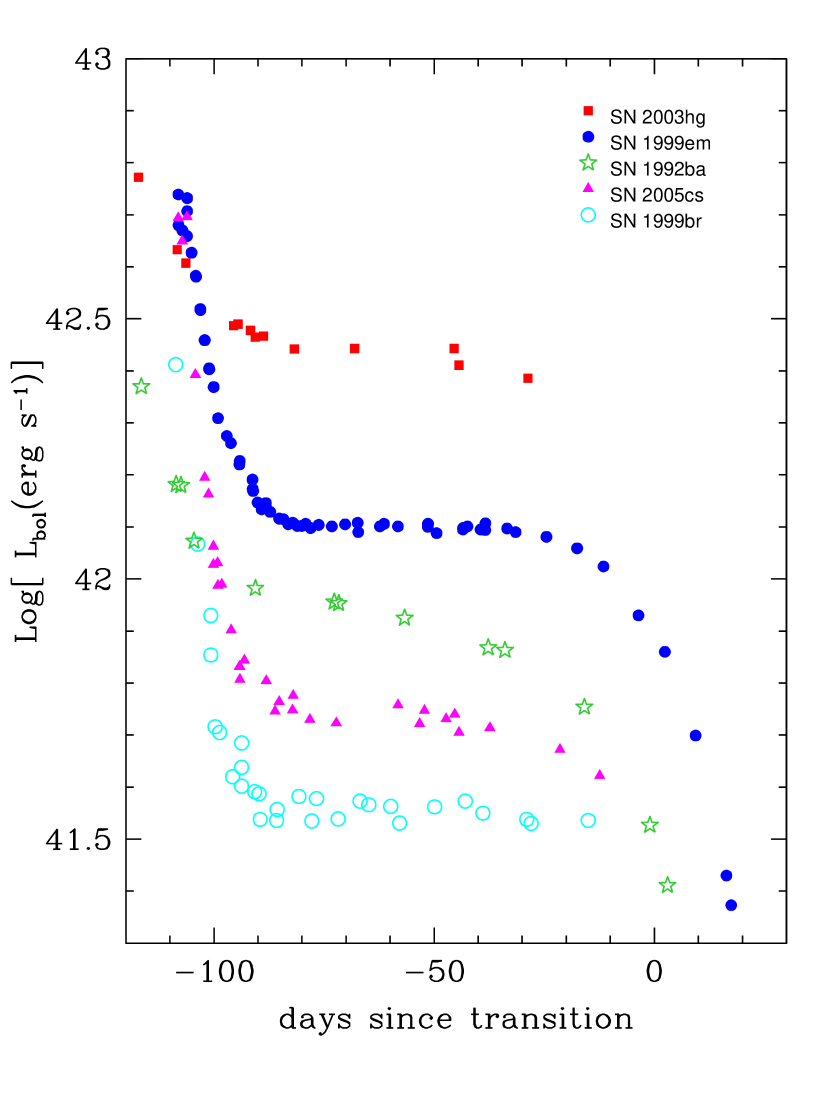
Figure 10: Bolometric light curves for five SNe of our sample showing the range of variation of the plateau luminosities.

A simple inspection of the resulting bolometric light curves of our sample reveals a high degree of heterogeneity among these SNe II-P which can be also seen in the subsample Figure 9. In Figure 10 we compare five exemplary SNe to illustrate the well known fact that SNe II-P display a wide range of plateau luminosities (Hamuy, 2001). The range of luminosities encompassed by our sample is $\sim$1 dex, equivalent to one order of magnitude of spread in their radiative energy output. The most frequent value of the plateau luminosity in our whole sample was $\sim 1.2\times 10^{42}$ erg s^-1.

There are 16 SNe with data previous to the plateau phase, i.e. during the adiabatic cooling phase. Among these, there are three subluminous objects, SN 1999br, SN 2003bl and SN 2005cs which, in comparison with the rest, appear to have a steeper slope during the adiabatic cooling phase and a flatter plateau (see Figure 10). In all cases where we observed a plateau where the luminosity remained nearly constant, or it slowly decreased, but it never increased. Utrobin (2007) has predicted that part of the dense core of the massive star should be ejected in order to produce a plateau phase as observed. On the contrary, if the whole core remains in the compact remnant and the density profile encountered by the shock wave in the envelope is relatively flat, the resulting luminosity increases with time. Our data suggest that all SN II-P ejecta involve part of the dense core of the progenitor star.

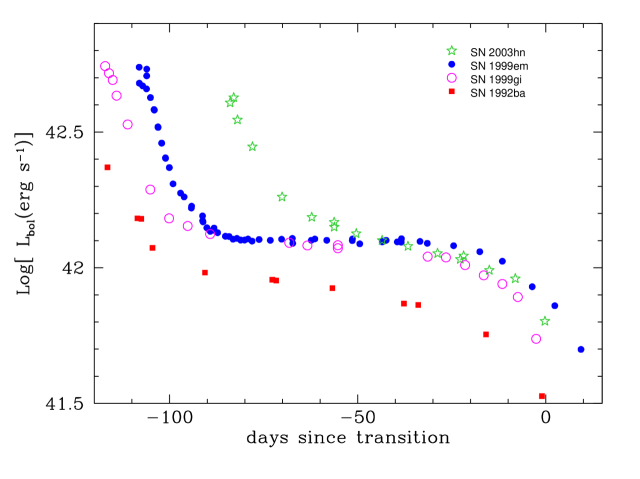
Figure 11: Bolometric light curves for four SNe of our sample showing the range of variation of the plateau lengths.

Twelve SNe with complete coverage between the adiabatic cooling phase and the transition to the radioactive tail showed a range of plateau durations between 75 and 120 days. In this study, we have defined the plateau phase as the part of the light curve on which the luminosity remains within 1 mag (or 0.4 dex) of the mean value calculated between 20 and 80 days before the epoch in the middle point of the transition to the radioactive tail (Olivares et al., 2009). Figure 11 shows a comparison of the light curves of four SNe selected to illustrate the variety of plateau lengths. It is known that the duration of the plateau is strongly related to the envelope mass of the progenitor object more than other parameters such as explosion energy and radius (Litvinova & Nadezhin, 1983; Popov, 1993). See for example the equation for the plateau duration ($t_{p}$) given by Popov (1993),$\;t_{p}\;\propto\;R^{1/6}E^{-1/6}M^{1/2}$ where R is the initial radius of the progenitor object, M is the ejected mass and E is the energy of the explosion. Based on this, our results indicate that there is a variety of envelope masses among the progenitors of SNe II-P. A quantitative assertion on this respect requires detailed modeling of the data.

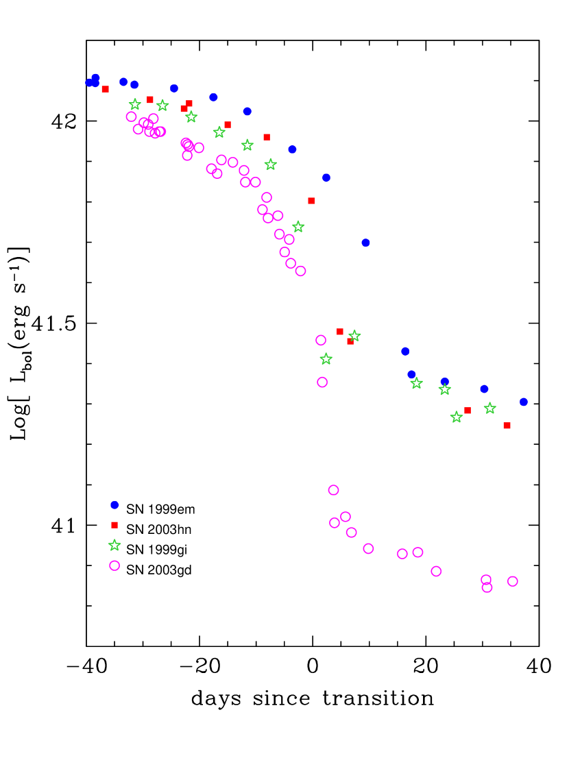
Figure 12: Bolometric light curves of four SNe of our sample with different transition properties.

Finally, we compared the shape of the transition between the plateau phase and the radioactive tail. Unfortunately, there are only six SNe for which this transition is well sampled. In Figure 12 we show this transition phase for four of the six SNe in this group. The luminosity drop is in the range of $\sim$ 0.8–1.12 dex. This behavior is related to the ⁵⁶Ni mass synthesized in the explosion and its degree of mixing. The amount of ⁵⁶Ni sinthetized by the SN determines the height of the radioactive tail. More ⁵⁶Ni mixing produces a more gradual transition between the plateau and the tail (Eastman et al., 1994; Utrobin, 2007). The drop for SN 2003gd appears to be steeper and larger than for the other SNe, which is indicative of less mixing and a smaller ⁵⁶Ni mass. From this preliminary study we can state that the ⁵⁶Ni mass produced and its mixing degree varies significantly among SNe II-P.

We are currently working on the determination of physical parameters for the progenitor stars of this sample of SNe using a hydrodynamical code recently developed by us (Bersten et al., 2009). The goal of that work, to be published soon, is to analyze the distribution of physical parameters for this sample of SNe II-P.

5 Conclusions

Using data from three SNe with excellent observations and two atmospheric models we derived reliable calibrations for bolometric corrections and effective temperature from $BVI$ photometry applicable to SNe II-P. The characteristic scatter of the BC calibration during the plateau phase is of 0.11 mag which corresponds to an uncertainty of 0.044 dex in bolometric luminosity. On the radioactive tail we found that the BC was independent of color with a value of $-0.70$ mag and a scatter of 0.02 mag based only on the behavior of SN 1987A. We noticed the importance of including $L$ and $M$ photometry in order to derive an accurate BC during this phase.

We emphasize that the largest uncertainties in our calibration of the BC occur at the earliest epochs corresponding to $(B-V)\lesssim 0.2$, where the discrepancies between models and data are the largest. During the rest of the SN evolution, we found an overall very good agreement between models and observations. A possible improvement to this calibration could be achieved from early spectra of SNe II-P in order to confirm the behavior shown by the models. In this sense it is important to note the recent suggestion by Gal-Yam et al. (2008) that the UV behavior of SNe II-P is very uniform. Another complication at early phases is the steep dependence of the BC on color. We point out that caution may be taken in the estimate of the extinction in order to use the BC to estimate luminosities at the earliest epochs. In this sense, the BC of the $(V-I)$ color appears to be less sensitive to extinction and therefore offers a better calibration at early epochs.

Regarding the effective temperature calibration, we found systematic differences between the two sets of models considered but we did not find any strong reason to rule out any of them. The characteristic scatter of the T_eff versus color calibration was $500$K for $(B-V)$ and $350$K for $(V-I)$ in the case of the E96 models, while for the D05 models it was $670$K for $(B-V)$ and $800$K for $(V-I)$.

Based on these calibrations we derived bolometric luminosities and effective temperatures for 33 SNe II-P, which prove a useful resource to extract physical properties of this type of objects. In this preliminary analysis we found that the SNe II-P in our sample showed a range of $\sim$ 1 dex in plateau luminosity (Lp) with most of the SNe having Lp $\sim 1.2\times 10^{42}$ erg s^-1. Plateau durations ranged between 75 and 120 days, which indicates the existence of a variety of ejected masses among SNe II-P. We also compared the shape of the transition between the plateau and the radioactive tail. We found that the size of the drop ranged between 0.8 and 1.12 dex indicating a variety of masses and degrees of mixing of ⁵⁶Ni for this SN sample.

Table 1: Coefficients of the fits to BC(color).

ai	$B-V$	$V-I$	$B-I$
a0	-0.823	-1.355	-1.096
a1	5.027	6.262	3.038
a2	-13.409	-2.676	-2.246
a3	20.133	-22.973	-0.497
a4	-18.096	35.542	0.7078
a5	9.084	-15.340	0.576
a6	-1.950	$\cdots$	-0.713
a7	$\cdots$	$\cdots$	0.239
a8	$\cdots$	$\cdots$	-0.027
ranges	$[-0.2,1.65]$	$[-0.1,1]$	$[-0.4,3]$
No. points	512	465	512
rms [mag]	0.113	0.109	0.091

Table 2: Coefficients of the fits to T_eff(color).

	$B-V$	$B-V$	$V-I$	$V-I$
ai	$E96$	$D05$	$E96$	$D05$
a0	0.790	0.884	0.957	1.106
a1	-1.856	-2.340	-2.254	-1.736
a2	4.055	6.628	5.922	-6.403
a3	-3.922	-8.456	-18.476	33.762
a4	1.368	4.619	36.058	-48.260
a5	$\cdots$	-0.849	-25.291	22.362
ranges	$[-0.2,1.15]$	$[-0.2,1.15]$	$[-0.1,0.65]$	$[-0.07,0.83]$
rms [K]	500	670	350	800

References

- Baron et al. (2000) Baron, E., et al. 2000, ApJ, 545, 444
- Bersten et al. (2009) Bersten, M., et al. 2009, in preparation
- Bouchet et al. (1989) Bouchet, P., Slezak, E., Le Bertre, T., Moneti, A., & Manfroid, J. 1989, A&AS, 80, 379
- Burrows (2000) Burrows, A. 2000, Nature, 403, 727
- Cappellaro et al. (2005) Cappellaro, E., et al. 2005, A&A, 430, 83
- Cardelli et al. (1989) Cardelli, J. A., Clayton, G. C., & Mathis, J. S. 1989, ApJ, 345, 245
- Chevalier & Soker (1989) Chevalier, R. A., & Soker, N. 1989, ApJ, 341, 867
- Chevalier et al. (2006) Chevalier, R. A., Fransson, C., & Nymark, T. K. 2006, ApJ, 641, 1029 Clayton, G. C., & Mathis, J. S. 1989, ApJ, 345, 245
- Dessart & Hillier (2005a) Dessart, L., & Hillier, D. J. 2005, A&A, 437, 667
- Dessart & Hillier (2005b) Dessart, L., & Hillier, D. J. 2005, A&A, 439, 671
- Dessart (2008) Dessart, L. 2008 private communication
- Eastman et al. (1994) Eastman, R. G., Woosley, S. E., Weaver, T. A., & Pinto, P. A. 1994, ApJ, 430, 300
- Eastman et al. (1996) Eastman, R. G., Schmidt, B. P., & Kirshner, R. 1996, ApJ, 466, 911
- Eldridge & Tout (2004) Eldridge, J. J., & Tout, C. A. 2004, MNRAS, 353, 87
- Elmhamdi et al. (2003) Elmhamdi, A., Chugai, N. N., & Danziger, I. J. 2003, A&A, 404, 1077
- Falk & Arnett (1977) Falk, S. W., & Arnett, W. D. 1977, ApJS, 33, 515
- Filippenko (1997) Filippenko, A. V. 1997, ARA&A, 35, 309
- Folatelli et al. (2006) Folatelli, G., et al. 2006, ApJ, 641, 1039
- Freedman et al. (2001) Freedman, W. L., et al. 2001, ApJ, 553, 47
- Gal-Yam et al. (2007) Gal-Yam, A., et al. 2007, ApJ, 656, 372
- Gal-Yam et al. (2008) Gal-Yam, A., et al. 2008, ApJ, 685, L117
- Grassberg et al. (1971) Grassberg, E. K., Imshennik, V. S., & Nadyozhin, D. K. 1971, Ap&SS, 10, 28
- Hamuy & Suntzeff (1990) Hamuy, M., & Suntzeff, N. B. 1990, AJ, 99, 1146
- Hamuy (2001) Hamuy, M. 2001, Ph.D. thesis, Univ. Arizona
- Hamuy & Pinto (2002) Hamuy, M., & Pinto, P. A. 2002, ApJ, 566, L63
- Hamuy (2003) Hamuy, M. 2003, ApJ, 582, 905
- Hamuy et al. (2009) Hamuy, M., et al. 2009, in preparation
- Heger et al. (2003) Heger, A., Fryer, C. L., Woosley, S. E., Langer, N., & Hartmann, D. H. 2003, ApJ, 591, 288
- Jones et al. (2009) Jones, M. I., et al. 2009, ApJ, 696, 1176
- Krisciunas et al. (2009) Krisciunas, K., et al. 2009, AJ, 137, 34
- Leonard & Filippenko (2001) Leonard, D. C., & Filippenko, A. V. 2001, PASP, 113, 920
- Leonard et al. (2002) Leonard, D. C., et al. 2002, AJ, 124, 2490
- Leonard et al. (2003) Leonard, D. C., Kanbur, S. M., Ngeow, C. C., & Tanvir, N. R. 2003, ApJ, 594, 247
- Litvinova & Nadezhin (1983) Litvinova, I. I., & Nadezhin, D. K. 1983, Ap&SS, 89, 89
- Litvinova & Nadezhin (1985) Litvinova, I. Y., & Nadezhin, D. K. 1985, Soviet Astronomy Letters, 11, 145
- Nadyozhin (2003) Nadyozhin, D. K. 2003, MNRAS, 346, 97
- Mannucci et al. (2005) Mannucci, F., Della Valle, M., Panagia, N., Cappellaro, E., Cresci, G., Maiolino, R., Petrosian, A., & Turatto, M. 2005, A&A, 433, 807
- Olivares et al. (2009) Olivares F., et al. 2009, in preparation
- Pastorello et al. (2006) Pastorello, A., et al. 2006, MNRAS, 370, 1752
- Popov (1993) Popov, D. V. 1993, ApJ, 414, 712
- Sahu et al. (2006) Sahu, D. K., Anupama, G. C., Srividya, S., & Muneer, S. 2006, MNRAS, 372, 1315
- Schlegel et al. (1998) Schlegel, D. J., Finkbeiner, D. P., & Davis, M. 1998, ApJ, 500, 525
- Shigeyama & Nomoto (1990) Shigeyama, T., & Nomoto, K. 1990, ApJ, 360, 242
- Smartt et al. (2004) Smartt, S. J., Maund, J. R., Hendry, M. A., Tout, C. A., Gilmore, G. F., Mattila, S., & Benn, C. R. 2004, Science, 303, 499
- Smartt et al. (2009) Smartt, S. J., Eldridge, J. J., Crockett, R. M., & Maund, J. R. 2009, MNRAS, 395, 1409
- Suntzeff & Bouchet (1990) Suntzeff, N. B., & Bouchet, P. 1990, AJ, 99, 650
- Tsvetkov et al. (2006) Tsvetkov, D. Y., Volnova, A. A., Shulga, A. P., Korotkiy, S. A., Elmhamdi, A., Danziger, I. J., & Ereshko, M. V. 2006, A&A, 460, 769
- Utrobin (2007) Utrobin, V. P. 2007, A&A, 461, 233
- Vinkó et al. (2006) Vinkó, J., et al. 2006, MNRAS, 369, 1780
- Woosley (1988) Woosley, S. E. 1988, ApJ, 330, 218
- Woosley et al. (1989) Woosley, S. E., Hartmann, D., & Pinto, P. A. 1989, ApJ, 346, 395