Ideal Stabilization

Abstract

We define and explore the concept of ideal stabilization. The program is ideally stabilizing if its every state is legitimate. Ideal stabilization allows the specification designer to prescribe with arbitrary degree of precision not only the fault-free program behavior but also its recovery operation. Specifications may or may not mention all possible states. We identify approaches to designing ideal stabilization to both kinds of specifications. For the first kind, we state the necessary condition for an ideally stabilizing solution. On the basis of this condition we prove that there is no ideally stabilizing solution to the leader election problem. We illustrate the utility of the concept by providing examples of well-known programs and proving them ideally stabilizing. Specifically, we prove ideal stabilization of the conflict manager, the alternator, the propagation of information with feedback and the alternating bit protocol.

1 Introduction

A program is self-stabilizing [8, 9, 20] (or just stabilizing) if, regardless of the initial state, it eventually satisfies its specification. This elegant property enables the program to recover from transient faults or lack of initialization. During this stabilization period the program behavior is unpredictable. It is tempting to attempt to engineer the specification such that the program behavior during fault-recovery is controlled. For example, the program starts behaving correctly in no more than ten steps, or critical messages are never lost. However, one of the features of classic stabilization is that the program does not have to satisfy the specification for an arbitrary amount of time. That is, the program is free to ignore the recovery constrains built into the specification.

Another disadvantage of stabilizing programs is their poor compositional properties. Stabilization programs are usually composed by layers: an lower level components are not influenced by the higher level components and, after the lower component starts behaving correctly, they higher level, due to stabilization will eventually behave correctly as well. However, if there is non-trivial two-way interaction between components, the stabilization or correct operation of the composed system is not guaranteed. These shortcomings diminish the attractiveness of stabilization as a viable fault-tolerance technique.

In this paper we study the class of programs that always satisfy their specification. We call such programs ideally stabilizing. Related concepts are periodically considered by fault-tolerance researchers. However, these approaches are often regarded as theoretical curiosity with a few isolated examples of no practical importance. Our thesis is that the opposite is true. Ideal stabilization retains most of the advantages of classical stabilization while allowing the engineers and program designers to control the program behavior during fault recovery. Moreover, since the ideally stabilizing programs always satisfy their specification, their composition is similar to conventional program composition. Thus, the vast array of established program composition techniques can be applied to ideally stabilizing programs. We are thus hopeful that our approach to stabilization makes the general concept of self-stabilization more attractive to fault-tolerance practitioners.

Related work.

Ideal stabilization is close to snap-stabilization [3, 6] and should be considered complementary. However, snap-stabilization is defined in terms of immediate correct satisfaction of external invocations. Such definition may lead to specifications with sequence-based safety and liveness properties. Proving stabilization to such specifications often results in operational proofs that are difficult to verify. Ideal stabilization, on the other hand, does not restrict specifications in any way.

Adding safety properties to self-stabilizing protocols has been a very active recent path of research, however most approaches make some restrictions on the nature or the extent of the faults in order to guarantee a particular kind of safety. Safe stabilization [12, 2] refers to the fact that few faults hitting the network should not compromise a particular safety predicate, while preserving global self-stabilization of the system. Also, the line of work about fault-containing stabilization [13] may handle only a single transient failure to ensure actual containment and recovery, and super-stabilizing protocols [10] can withstand one topology change at a time. When faults are simple enough to be detected by checksums [16], it is also possible to maintain elaborate safety predicates. Other approaches included using external entities that enforce safety [11] or make use of non-corruptible memory [18]. By contrast, ideal stabilization does not restrict the nature or the extent of the transient faults that can hit the system in any way, and does not make use of any external entity.

Our contribution.

In this paper we study two approaches to ideal stabilization. The approaches depend on the specification type. Specification itself is ideal if it allows (i.e. mentions) all possible states. Specification is not ideal otherwise. Ideal stabilization to specifications that are not ideal hinges on the approach we call state displacement. The specification implementer provides such mapping from program states to specification states that none of the possible program states map to disallowed specification states. We identify the necessary condition for such specifications to allow ideal stabilization and explain how two well-known programs: conflict manager and the alternator use state displacement to achieve ideal stabilization.

The second approach relies on stating the specification such that all the possible states are allowed. This allows the engineer to specify precisely what behavior, including failure recovery behavior, is expected of the program. Ideally stabilizing program, by definition, has to follow this specification exactly. We state a proposition that states that such programs are rather common. As an example, we consider the problem specifications for two well-known stabilizing programs: propagation of information with feedback and alternating-bit protocol and provide assertional proofs that the programs ideally stabilize to these specifications.

2 Model

This section introduces the notation and terms we use in the rest of the paper. To the person familiar with the literature on self-stabilization, our notation may look fairly conventional. However, we encourage even the specialists to read this section as the understanding of the results in the further sections hinges on the notions defined in this one.

Program. A program consists of a set of $N$ processes. Each process contains a set of variables. Every variable ranges over a fixed domain of values. Variable $v$ of process $p$ is denoted $v.p$. A process state is an assignment of a value from its domain to each variable of the process. A program state, in turn, is an assignment of a value to every variable of each process. The Cartesian product of the values of all program variables is program state universe. That is, the state universe defines all states that the program can assume.

Each process also contains a set of actions. An action has the form $\langle name\rangle:\langle guard\rangle\longrightarrow\langle command\rangle$. A guard is a predicate over the variables of the process. A command is a sequence of assignment and branching statements.

An action whose guard is true at some program state is enabled in that state. The execution of an enabled action changes the values of program variables and thus transitions the program from one state to another. A program computation is a maximal sequence of such transitions. By maximality we mean that the computation is either infinite or it ends in a state where none of the actions are enabled. Note that we do not assume any fairness of action execution for infinite computations.

Communication model, extended state. Processes that share variables are neighbors. The communication model determines the type and access method of the variables shared by neighbor processes. For example, in shared-memory communication model, the process may mention the variables of the neighbor processes in its actions. That is, the process may read the state of its neighbor processes. The extended state of the process is the state of its local variables and the variables that the process can read.

Problem specifications and program sequence mapping. Problem specification prescribes the program behavior. This is done by defining the program inputs and outputs through external variables. External variables are thus either input or output variables. Input variables are modified by the environment while the program may only read them. The output variables are updated by the program, they are used to display the results of the program computation.

The problem specification is the set of sequences of states of external variables. A program implements the specification. Part of the implementation is the mapping from the program states to the specification states. This mapping does not have to be one-to-one. However, we only consider unambiguous programs where each program state maps to only one specification state.

We make another important assumption about program sequence mappings. The mappings have to be merge-symmetric. Specifically, let there be a set of program states $pr_{1}$ through $pr_{k}$ such that they map to specification states $s_{1}$ through $s_{k}$. Then, if there is a specification state $s_{m}$ such that the extended state of each process $p$ in $s_{m}$ is the same as in one of the states $s_{1}$ through $s_{k}$, then there exists a program state $pr_{m}$ that maps to $s_{m}$. In other words, any specification state formed by extended process state-preserving combination of other specification states, has a program state that maps to this new specification state. Most known mappings are merge-symmetric.

Identical mapping maps every program state to the specification state. That is, the program operates external variables only. Another simple program mapping is projection. Each process maintains output variables and internal variables for computations and record keeping. The projection of program states onto specification states removes the internal variables. However, the mapping may not be as straightforward as identical mapping or projection. For example, the specification requires the output variable of a process be boolean while the program maintains an integer variable. The mapping is such that the even values of the integer variable are mapped to true while odd values to false.

Once the mapping between program and specification states is established, the program computations are mapped to specification sequences as follows. Each program state is mapped to the corresponding specification state. Then, stuttering, the consequent identical specification states, is eliminated.

The program does not have to implement all specification sequences. However, the program cannot select implementation sequences so that it ignores environment input. Hence the following notion of input completeness. Given a set of sequences ${\cal A}$, a subset ${\cal B}\subset{\cal A}$ is input-complete if, for every sequence $\alpha\in{\cal A}$, there exists a sequence $\beta\in{\cal B}$ such that: every step $s_{1}$ of $\alpha$ is also in $\beta$ and for every pair of steps $s_{1}$ and $s_{2}$ their order in $\alpha$ and $\beta$ is the same. Informally, the sequences in an input-complete subset ${\cal B}$ preserve the results and the order of the input steps in ${\cal A}$.

The state universe of the specification is the Cartesian product of the values of all the external variables. The state that is present in one of the specification sequences is allowed by the specification. The state is disallowed otherwise. The specification is ideal if it allows every state in its state universe; otherwise the specification is not ideal.

We only consider specifications that are suffix-closed. That is, every suffix of a specification sequence is also a sequence in this specification. Suffix closure enables us to discuss the correctness of the program on the basis of its current state rather than potentially arbitrary long program history. This facilitates assertional reasoning about program correctness.

Predicates, invariants, stabilization. A state predicate is a boolean expression over program variables. A program state conforms to predicate $R$, if $R$ evaluates to true in this state; otherwise, the state violates $R$. By this definition every state in the program state universe conforms to predicate true and none conforms to false.

The predicate defines a set of program states that conform to it. In the sequel we use the predicate and the set of states it defines interchangeably. Predicate $R$ is closed in a certain program ${\cal P}$, if every state of every computation of ${\cal P}$ conforms to $R$ provided that the computation starts in a state conforming to $R$.

A closed predicate $I$ is an invariant of the program ${\cal P}$ with respect to specification ${\cal S}$ if $I$ has the following property: every computation of ${\cal P}$ that starts in a state conforming to $I$, maps to a sequence that belongs to the specification. A program state is legitimate if it conforms to the invariant and illegitimate otherwise.

Program ${\cal P}$ satisfies (or solves) specification ${\cal S}$, if there exists an invariant $I$ of ${\cal P}$ with respect to ${\cal S}$ such that the mappings of the program computations that start from $I$ form an input-complete subset of ${\cal S}$. That is, the program does not have to implement all the specification sequences, but it does need to accommodate all possible inputs. Specifically, it needs to implement an input-complete subset of these sequences.

A program ${\cal P}$ is stabilizing to specification ${\cal S}$ if every computation that starts in an arbitrary state of the program sate universe contains a state conforming to the invariant with respect to ${\cal S}$. Therefore, any computation of a stabilizing program contains a suffix that implements a specification sequence.

Definition 1

A program is ideally stabilizing if every state in its state universe is legitimate.

That is, true is an invariant of an ideally stabilizing program.

3 State Displacement

3.1 Necessary Condition for Specification

A non-ideal specification disallows certain states in its state universe. Yet, every state in the program state universe is legitimate. Thus, for a program to ideally stabilize to such specification, the state mapping should be such that the disallowed states are displaced. That is, none of the states in the program state universe maps to the disallowed states. However, state displacements may not be possible for an arbitrary specification. In this section we provide a theorem that establishes a necessary condition for a specification to be solvable by an ideally-stabilizing program.

Theorem 3.1

An ideal stabilization is possible to non-ideal specification only if the specification contains an input-complete subset of sequences such that in every disallowed specification state there is at least one process whose extended state does not occur in any of the specification states of this subset.

Proof:Assume the opposite. There is, a non-ideal specification ${\cal S}$ that disallows state $d$ and for every input-complete subset ${\cal C}$ of ${\cal S}$ and for every process $p_{i}$, where $i=1,N$, there is a specification state $c_{i}$ in one of the sequences of ${\cal C}$ such that the extended state of $p_{i}$ is the same in $c_{i}$ and in $d$. However, there is a program ${\cal P}$ that ideally stabilizes to ${\cal S}$.

Since ${\cal P}$ solves ${\cal S}$, ${\cal P}$ implements an input complete-subset of ${\cal S}$. Assume, without loss of generality, that ${\cal P}$ implements ${\cal C}$. That is, for every sequence of ${\cal C}$ there is a computation of ${\cal P}$ that maps to this sequence. This means that for each specification state of ${\cal C}$, there is a program state of ${\cal P}$ that maps to it. This includes the states $c_{i}$. For each $i$, let $pr_{i}$ be the program state of ${\cal P}$ that maps to $c_{i}$.

Recall that the extended state of each process in $d$ is the same as in one of the states $c_{i}$. If this is the case then, according to merge-symmetry of program mapping, there exists are program state $pr_{d}$ that maps to $d$. Let us consider the computation of ${\cal P}$ that starts in $pr_{d}$. This computation contains a state that maps to a disallowed state, $pr_{d}$ itself. That is, this computation maps to a sequence outside the specification ${\cal S}$. This means that $d$ does not conform to an invariant of ${\cal P}$ with respect to ${\cal S}$. That is, $pr_{d}$ is an illegitimate state. However, if ${\cal P}$ has an illegitimate state then, contrary to our initial assumption, ${\cal P}$ does not ideally stabilize to ${\cal S}$. Hence the theorem. $\Box$

3.2 Examples

To illustrate the concept of ideal stabilization to non-ideal specifications and the ramifications of Theorem 3.1, we provide several examples.

Conflict manager. The specification we consider is a simplified (unfair) variant of the dining philosophers problem [4, 7] that we call ${\cal UDP}$. The program is adapted from the deterministic conflict manager presented by Gradinariu and Tixeuil [15]. The processes are arranged in a chain. Every process has a unique identifier. The specification defines one external output boolean variable $in$ per process. If the value of $in$ is true, the process may execute the exclusive critical section of code. The specification defines infinite sequences where $in$ variables alternate between true and false. The sequences are not necessarily fair as a certain process may never be given a chance to execute the crucial section. That is, an input-complete subset of the specification contains any subset of such sequences.

The specification prohibits concurrent critical section access by neighbor processes. That is, the specification disallows states where $in$ variables of two neighbors are true in the same state. Assuming shared memory communication, the extended state of the process contains the state of its neighbors. Hence, none of the allowed specification states contain an extended process state where both the process and one of its neighbors are inside the critical section. The specification thus satisfies the conditions of Theorem 3.1.

The conflict manager program ${\cal CM}$ is as follows. Each process has a single boolean variable access and a single action flip that is always enabled. The action toggles the value of access.

$$\emph{flip}:\textbf{true}\longrightarrow access:=\neg access$$

The program mapping is this. For each process $p$ the variable $p.in$ is true if $p.access$ is true and $p$ has the highest identifier among its neighbors with $access$ set to true.

Let us discuss why this mapping is merge-symmetric. Any extended process state-preserving combination of specification states produces a specification state where neighbors are not accessing the critical section. Then, by appropriately setting $access$ variables, we can generate the program state that maps to this specification state.

Let us give an illustration for this reasoning. Assume we have a chain of four processes with identifiers $\langle 2,1,3,4\rangle$. The extended state of each process in this case is its own state plus the state of its left and right neighbors. Consider two specification states

$$s_{1}\equiv\langle\textbf{true},\textbf{false},\textbf{false},\textbf{false}\rangle$$

and

$$s_{2}\equiv\langle\textbf{false},\textbf{false},\textbf{false},\textbf{true}\rangle$$

Some of the program states that map to $s_{1}$ and $s_{2}$ are respectively $pr_{1}\equiv\langle\textbf{true},\textbf{true},\textbf{false},\textbf{false}\rangle$ and $pr_{2}\equiv\langle\textbf{false},\textbf{false},\textbf{false},\textbf{true}\rangle$.

Specification state $s_{3}\equiv\langle\textbf{true},\textbf{false},\textbf{false},\textbf{true}\rangle$ is formed by merging states $s_{1}$ and $s_{2}$. Note that the extended states of each process in $s_{3}$ are the same in either $s_{1}$ or $s_{2}$. For example, the extended state of process $p_{2}$ is $\langle\textbf{true},\textbf{false},\textbf{false}\rangle$, which is the same in $s_{1}$ and $s_{3}$. Note that there are a number of program states that map to $s_{3}$. For example, $pr_{3}\equiv\langle\textbf{true},\textbf{false},\textbf{false},\textbf{true}\rangle$.

Theorem 3.2

Program ${\cal CM}$ ideally stabilizes to the unfair dining philosophers specification ${\cal UDP}$.

Proof:To prove ideal stabilization we need to show that a computation of ${\cal CM}$ from an arbitrary program state satisfies ${\cal UDP}$. First, we show that every state of ${\cal CM}$ maps to an allowed state of ${\cal UDP}$. Indeed, among the neighbors whose $access$ is true, $in$ is set to true only for the process with the highest identifier. That is, every program state maps to the state of ${\cal UDP}$ where neighbors do not access the critical section concurrently. Hence, no program state maps to a disallowed state.

Moreover in every computation of the program at least one process, the process with the largest identifier in the system, alternates between setting access to true and false. This means that this process alternates between entering and exiting the CS indefinitely. Such computations satisfy the specification. That is, ${\cal CM}$ ideally stabilizes to ${\cal UDP}$. $\Box$

Leader election. We show a simplified leader election problem ${\cal LE}$ as an example of the specification to which ideally stabilizing solutions do not exist. Again, the processes form a chain. In this case, we only consider $N>3$. In the external state, each process has two boolean variables: an input variable $contend$ and an output variable $leader$. The value of the input variable $contend$ is set to a particular value and does not change throughout the specification sequence. In each specification state $leader$ of at most one process is true. To exclude trivial solutions, the specification requires that the leader is elected only out of the processes that contend for leadership. That is, the processes whose $contend$ variable is true. Each specification sequence is finite and ends with a state where the leader is elected. Note that the input complete subset of sequences has to contain a sequence for every combination of the contending processes.

Theorem 3.3

There does not exist a program that ideally stabilizes to the simplified leader election specification ${\cal LE}$.

Proof:Let us consider state $s_{1}$ where the first process is the only one contending for leadership. This is the process that has to be elected leader. That is, the following output state has to be in every input-complete subset. $s_{1}\equiv\langle\textbf{true},\textbf{false},\cdots,\textbf{false},\textbf{false}\rangle$ Similarly, let $s_{2}$ be the state where the last process is the only one contending: $s_{2}\equiv\langle\textbf{false},\textbf{false},\cdots,\textbf{false},\textbf{true}\rangle$.

We now form the state $s_{3}$ where both the first and the forth processes are contending for leadership and both of them are elected. That is,

$$s_{3}\equiv\langle\textbf{true},\textbf{false},\cdots,\textbf{false},\textbf{true}\rangle$$

This state is disallowed . Yet, the extended state of every process is present in either $s_{1}$ or $s_{2}$. Thus, according to Theorem 3.1, ideal stabilization is not possible to ${\cal LE}$. $\Box$

Linear alternator. For another example, we demonstrate how a well-known program called the linear alternator ${\cal LA}$ proposed by Gouda and Haddix [14] fits into our ideal stabilization model. The alternator provides a solution to the fair variant of the dining philosophers problem ${\cal FDP}$. The problem specification is the same as described above except all the sequences are fair with respect to the process critical section access. The modified specification still excludes the states where two neighbors are executing the critical section concurrently and the specification still satisfies the conditions of Theorem 3.1. Therefore, the ideal solution is still possible for this specification.

The implementation of ${\cal LA}$ is as follows. Similar to ${\cal CM}$ manager, each process has a boolean variable $x$. This time though we assume that the processes in the chain are numbered in the increasing order from $1$ to $N$. The numbering is for presentation purposes only as as each process only need to be aware of its right and left neighbor. The process actions are as follows. In the actions, parameter $j$ ranges from $2$ to $N-1$.

$$\begin{array}[]{lll}x.p_{1}=x.p_{2}&\longrightarrow&x.p_{1}:=\neg x.p_{1}\\ (x.p_{j}\neq x.p_{j-1})\wedge(x.p_{j}=x.p_{j+1})&\longrightarrow&x.p_{j}:=\neg x.p_{j}\\ x.p_{N-1}\neq x.p_{N}&\longrightarrow&x.p_{N}:=\neg x.p_{N}\end{array}$$

The program to specification states mapping is as follows. For each process $p_{j}$, the output variable $in.p_{j}$ evaluates to true if process’ action is enabled.

Theorem 3.4

Program ${\cal LA}$ ideally stabilizes to the fair dining philosophers specification ${\cal FDP}$.

Proof:

Gouda and Haddix [14] prove that the alternator satisfies the fairness properties of the dining philosophers specification from an arbitrary program state. We only show the displacement of disallowed states. Note that an action of a process $p$ is enabled if $x.p$ is not equal to the left neighbor’s variable and equal to the right neighbor’s variable. This can only hold for one process in the neighborhood. That is, every program state maps to a specification state where none of the neighbors are in the critical sections concurrently. In other words, the program states only map to the allowed states. Hence the theorem. $\Box$

4 Stabilizing to Ideal Specifications

4.1 Forming Ideal Specifications

Another method of achieving ideal stabilization is by stating the specification such that all the states in its universe are legitimate. That is, stating ideal specification. At first sight this seems difficult to achieve. However, the following proposition demonstrates that such specifications are rather common.

Proposition 1

For every program there is an ideal specification to which this program ideally stabilizes.

We provide an informal argument for the validity of this proposition. Consider any program and all the computations produced by this program when it starts from an arbitrary state of its universe. Now define the specification that contains exactly these computations. This specification is ideal as all the states of its state universe are allowed while the program ideally stabilizes to this specification.

Naturally, this kind of specification may not be very useful as it, in essence, defines specification to be whatever the program computes. However, below we describe how a number of stabilizing program published in the literature can be defined as ideally stabilizing to ideal specifications.

4.2 Examples

Propagation of Information with Feedback. As the first example we describe a program ${\cal PIF}$ that ideally stabilizes to the propagation of information with feedback [5, 19] specification. The presentation of this program as snap-stabilizing is well-known [3]. The program is presented on rooted trees. However, to simplify the presentation, we describe the operation of this program on a chain.

For ease of exposition we preserve the rooted tree terminology. Similarly to the alternator, we assume that the processes are numbered from $1$ to $N$ from left to right in the chain. We refer to the leftmost processor, with identifier $1$, as root; the rightmost, with identifier $N$, as leaf; and the processes in between as intermediate. For each process $p$, the processes to the left of it are ancestors and to the right — descendants.

Each process has a state variable $st$. In the intermediate processes, the variable may hold one of the three values: i, rq, rp which stand for idle, requesting and replying respectively. The root can only be idle or requesting while the leaf can be either idle or replying.

The objective of the program is to send a signal from the root to the leaf and in return receive an acknowledgment that matches this signal. Operationally, the program should ensure that after the root makes a request then every process propagates this request along the chain from left to right in causally ordered steps transitioning from idle to requesting. Afterwards, the processes propagate the reply from right to left in causally ordered steps transitioning from requesting to replying.

We define the following state predicates. $RP(k)$ are the specification states where all $k$ processes on the left are requesting $(k=1,N-1)$ and the rest of the processes are replying. $RQ(l,m)$ are the specification states where all $l$ processes on the left are requesting $(l=0,N-1)$ and all $m-l$ processes following them are idle $(m=l+1,N)$ while the remaining processes are replying. Specification ${\cal SPIF}$ includes the sequences where the system satisfies one of the predicates and transitions from one to the other infinitely.

Let us define another pair of predicates. Predicate $RP^{\prime}(k)$ defines the states where $k$ processes on the left are requesting $(k=1,N-1)$, the process $k+1$ is replying and none of the rest are idle. Notice that $RP(k)\subset RP^{\prime}(k)$. Predicate $RQ^{\prime}(l,m)$ are the states where all $l$ processes on the left are requesting $(l=0,N-1)$, all $m-1$ following them are idle $(m=l+1,N)$ and the state of the other processes is arbitrary. Similarly, $RQ(l,m)\subset RQ^{\prime}(l,m)$. Specification ${\cal IPIF}$ includes the sequences where the system always satisfies either $RP^{\prime}(k)$ or $RQ^{\prime}(l,m)$, each sequence has a sequence in ${\cal SPIF}$ as a suffix and the transition from $RQ^{\prime}(l,m)$ is only to $RP(k)$.

We now describe program ${\cal PIF}$. It has only external variables. The mapping between the program and specification variables is identical. The actions of ${\cal PIF}$ are shown in Figure 1.

$$\begin{array}[]{llllllll}\emph{request}:&&&st.p_{1}=\textbf{i}&\wedge&st.p_{2}=\textbf{i}&\longrightarrow&st.p_{1}:=\textbf{rq}\\ \emph{clear}:&&&st.p_{1}=\textbf{rq}&\wedge&st.p_{2}=\textbf{rp}&\longrightarrow&st.p_{1}:=\textbf{i}\\ \emph{forward}:&st.p_{j-1}=\textbf{rq}&\wedge&st.p_{j}=\textbf{i}&\wedge&st.p_{j+1}=\textbf{i}&\longrightarrow&st.p_{j}:=\textbf{rq}\\ \emph{back}:&st.p_{j-1}=\textbf{rq}&\wedge&st.p_{j}=\textbf{rq}&\wedge&st.p_{j+1}=\textbf{rp}&\longrightarrow&st.p_{j}:=\textbf{rp}\\ \emph{stop}:&st.p_{j-1}=\textbf{i}&\wedge&st.p_{j}\neq\textbf{i}&&&\longrightarrow&st.p_{j}:=\textbf{i}\\ \emph{reflect}:&st.p_{N-1}=\textbf{rq}&\wedge&st.p_{N}=\textbf{i}&&&\longrightarrow&st.p_{N}:=\textbf{rp}\\ \emph{reset}:&st.p_{N-1}=\textbf{i}&\wedge&st.p_{N}=\textbf{rp}&&&\longrightarrow&st.p_{N}:=\textbf{i}\end{array}$$

Figure 1: ${\cal PIF}$ program actions. Actions request and clear belong to the root process; actions forward, back, and stop – to intermediate processes, i.e parameter $j$ ranges from $2$ to $N-1$; actions reflect and reset – to the leaf.

Theorem 4.1

${\cal PIF}$ classically stabilizes to ${\cal SPIF}$ and ideally stabilizes to ${\cal IPIF}$.

Proof:First, we prove that $RQ(l,m)\vee RP(k)$ is an invariant of ${\cal PIF}$ with respect to ${\cal SPIF}$. Notice that this disjunction is closed in ${\cal PIF}$. That is, none of the actions of ${\cal PIF}$ violate the predicate. Let us show that a program transitions from $RQ(l,m)$ to $RP(k)$ and back. If the program satisfies $RQ(l,m)$, at least one action is enabled. Indeed, if $l=0,m<N$, request is enabled in stop is enabled in process $p_{m+1}$. If, $l<m-1,m\leq N$, request is enabled in $p_{l+1}$. With the execution of an action either $l$ or $m$ are incremented. If $l=N-1,m=N$, reflect is enabled that transitions the program into $RP(N-1)$. Similarly, if the system satisfies $RP(k)$ for $k=2,N-1$, action back is enabled. The execution of this action keeps the system in $RP(k)$ but decrements $k$. If $k=1$, clear is enabled. Its execution moves the program back in $RQ(l,m)$. That is, the disjunction of the two predicates is closed and a ${\cal PIF}$ computation that starts in a state conforming to one of them, satisfies ${\cal SPIF}$. Hence, $RQ(l,m)\vee RP(k)$ is an invariant of ${\cal SPIF}$.

Observe that the disjunction of $RQ^{\prime}(l,m)\vee RP^{\prime}(k)$ contains the program, as well as specification, state universe. We show that ${\cal PIF}$ stabilizes to ${\cal SPIF}$ from this predicate as required by ${\cal IPIF}$. An argument similar to the above demonstrates that an action is enabled if ${\cal PIF}$ satisfies $RP^{\prime}(k)$. This action either decrements $k$ or moves the system to $RQ^{\prime}(l,m)$. Also, similarly, if ${\cal PIF}$ satisfies $RQ^{\prime}(l,m)$, then an action is enabled that increments either $l$ or $m$. Moreover, if $l=N-1,m-N$, the execution of reflect transitions the system to $RP(k)$. That is, ${\cal PIF}$ moves from $RP^{\prime}(k)$ to $RQ^{\prime}(l,m)$ to $RP(k)$. This means that the program stabilizes to ${\cal SPIF}$ and ideally stabilizes to ${\cal IPIF}$. $\Box$

Alternating bit protocol. Alternating bit protocol is an elementary data-link network protocol. There is a number of classic stabilizing implementations of the protocol. Refer to Howell et al [17] for an extensive list of citations. There is also a snap-stabilizing version [6].

The problem is stated as follows. There are two processes: sender — $p$, and receiver — $q$. The processes maintain boolean sequence numbers $ns.p$ and $nr.q$. The processes exchange messages over communication channels. The channels are reliable and their capacity is one. That is, if the channel is empty, the message is reliably sent. If the channel already contains a message, an attempt to send another message leads to the loss of the new message. The processes exchange two types of messages: $data$ and $ack$. Both carry the sequence numbers.

Specification ${\cal SABP}$ prescribes infinite sequences of states where there is exactly one message in the channels. The message carries the sequence number of the sender. The state transitions are such that $p$ changes the value of $ns$. This change is followed by the change of the value in $nr$ that matches the value of $ns$.

Specification of ${\cal IABP}$ is such that for every state in the universe there is a sequence that starts in it and every sequence contains a sequence of ${\cal SABP}$ as a suffix. Specification of ${\cal IABP}$ is thus ideal.

The program ${\cal ABP}$ uses only external variables as described by ${\cal SABP}$ and ${\cal IABP}$. ${\cal ABP}$ actions are shown in Figure 3. The sender has two actions: next and timeout. Action next is enabled if there is a message from $q$ in the channel. The timeout action is enabled if there are no messages in either channel. Upon receiving a message from $q$ with matching sequence number, $p$ increments the sequence number and sends the next message. If $p$ times out, it resubmits the same message. The receiver has a single action. When $q$, receives a message, it sends an acknowledgment back to $p$. If the message bears a sequence number different from $rn$, $q$ increments $rn$ signifying the successful receipt of the message.

next:	$\textbf{receive}\ ack(nm)\longrightarrow$
		$\textbf{if}\ nm=ns\ \textbf{then}$
			$ns:=\neg ns$
			$\textbf{send}\ data(ns)$
timeout:	$\textbf{timeout}()\longrightarrow\textbf{send}\ data(ns)$
reply:	$\textbf{receive}\ data(nm)\longrightarrow$
		$\textbf{if}\ nm\neq nr\ \textbf{then}$
			$nr:=nm$
		$\textbf{send}\ ack(nm)$

Figure 2: ${\cal ABP}$ actions.

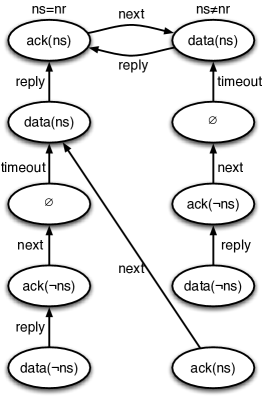
Figure 3: ${\cal ABP}$ state transitions.

Theorem 4.2

${\cal ABP}$ classically stabilizes to ${\cal SABP}$ and ideally stabilizes to ${\cal IABP}$.

Proof:We prove the correctness of the theorem by enumerating the state transitions of ${\cal PIF}$. We classify the state universe of ${\cal ABP}$ into two groups: (i) $ns$ is equal to $nr$ and (ii) $ns$ is not equal to $nr$. The states are further classified according to the type of messages in the channels. The states and state transitions are shown in Figure 3. Note that to simplify the diagram we do not show the states that contain more than a single message. However, after a single transition, the program moves from one of those states to a state shown in the figure. The correctness of the theorem claims can be ascertained by examining the states and transitions shown in the figure. $\Box$

5 The Impact of Ideal Stabilization Approach

In this paper we proposed a new way of approaching stabilization. Our approach eliminates two of the most problematic features of classic stabilization: unpredictable behavior during stabilization and poor composability. We hope that this work adds more credence to stabilization as a viable fault-tolerance technique and generates more interest in the subject among both theoretical researches and reliability engineers.

References

- [1] Anish Arora, editor. 1999 ICDCS Workshop on Self-stabilizing Systems, Austin, Texas, June 5, 1999, Proceedings. IEEE Computer Society, 1999.
- [2] Alina Bejan, Sukumar Ghosh, and Shrisha Rao. An extended framework of safe stabilization. In David Jeff Jackson, editor, Computers and Their Applications, pages 276–282. ISCA, 2006.
- [3] Alain Bui, Ajoy Kumar Datta, Franck Petit, and Vincent Villain. State-optimal snap-stabilizing pif in tree networks. In Arora [1], pages 78–85.
- [4] K.M. Chandy and J. Misra. The drinking philosophers problem. ACM Transactions on Programming Languages and Systems, 6(4):632–646, October 1984.
- [5] Ernest J. H. Chang. Echo algorithms: Depth parallel operations on general graphs. IEEE Transactions on Software Engineering, 8(4):391–401, July 1982.
- [6] Sylvie Delaët, Stéphane Devismes, Mikhail Nesterenko, and Sébastien Tixeuil. Brief announcement: Snap-stabilization in message-passing systems. In Principles of Distributed Computing (PODC 2008), August 2008.
- [7] E. Dijkstra. Cooperating Sequential Processes, pages 43–112. Academic Press, 1968.
- [8] Edsger W. Dijkstra. Self-stabilizing systems in spite of distributed control. Commun. ACM, 17(11):643–644, 1974.
- [9] S. Dolev. Self-stabilization. MIT Press, March 2000.
- [10] Shlomi Dolev and Ted Herman. Superstabilizing protocols for dynamic distributed systems. Chicago J. Theor. Comput. Sci., 1997, 1997.
- [11] Shlomi Dolev and Frank A. Stomp. Safety assurance via on-line monitoring. Distributed Computing, 16(4):269–277, 2003.
- [12] Sukumar Ghosh and Alina Bejan. A framework of safe stabilization. In Shing-Tsaan Huang and Ted Herman, editors, Self-Stabilizing Systems, volume 2704 of Lecture Notes in Computer Science, pages 129–140. Springer, 2003.
- [13] Sukumar Ghosh, Arobinda Gupta, Ted Herman, and Sriram V. Pemmaraju. Fault-containing self-stabilizing algorithms. In Proceedings of the Fifteenth Annual ACM Symposium on Principles of Distributed Computing, pages 45–54, 1996.
- [14] Mohamed G. Gouda and F. Furman Haddix. The alternator. In Arora [1], pages 48–53.
- [15] Maria Gradinariu and Sébastien Tixeuil. Conflict managers for self-stabilization without fairness assumption. In Proceedings of the International Conference on Distributed Computing Systems (ICDCS 2007), page 46. IEEE, June 2007.
- [16] Ted Herman and Sriram V. Pemmaraju. Error-detecting codes and fault-containing self-stabilization. Inf. Process. Lett., 73(1-2):41–46, 2000.
- [17] Rodney R. Howell, Mikhail Nesterenko, and Masaaki Mizuno. Finite-state self-stabilizing protocols in message-passing systems. In Arora [1], pages 62–69.
- [18] Chengdian Lin and Janos Simon. Observing self-stabilization. In PODC, pages 113–123, 1992.
- [19] A. Segall. Distributed network protocols. IEEE Transactions on Information Theory, 29(2):23–35, January 1983.
- [20] Sébastien Tixeuil. Algorithms and Theory of Computation Handbook, Second Edition, chapter Self-stabilizing Algorithms. Chapman & Hall/CRC Applied Algorithms and Data Structures. Taylor & Francis, 2009.