Interacting non-minimally coupled canonical, phantom and quintom models of holographic dark energy in non-flat universe

Abstract

Motivated by our recent work [26], we generalize this work to the interacting non-flat case. Therefore in this paper we deal with canonical, phantom and quintom models, with the various fields being non-minimally coupled to gravity, within the framework of interacting holographic dark energy. We employ the holographic model of interacting dark energy to obtain the equation of state for the holographic energy density in non-flat (closed) universe enclosed by the event horizon measured from the sphere of horizon named $L$.

1 Introduction

Recent astrophysical data [1] strongly indicate that the universe is accelerating at present. Therefore, it is of paramount importance to explain why this is happening. Many theories have been proposed recently that try to address this issue, which has become the most important problem in cosmology. Although theories that try to modify Einstein equations [2] constitute a big part of these attempts, the mainstream explanation for this problem, however, is known as theories of dark energy. The most accepted idea indicates that a mysterious dominant component, dubbed dark energy, which has negative pressure, leads to this cosmic acceleration, though its nature and cosmological origin still remain unknown.

The combined analysis of the cosmological observations suggests that the universe consists of about $70\%$ dark energy, $30\%$ dust matter (cold dark matter plus baryons), and a negligible percentage of radiation. Although little about dark energy is known, we can still propose some candidates to describe it. The most natural candidate to account for this acceleration is the cosmological constant, by given the problems associated with it we turn our attention to dynamical dark energy models. The dynamical nature of dark energy, at least at an effective level, can be originated from various fields, such as a canonical scalar field (quintessence) [3], a phantom field, that is, a scalar field with a negative sign of the kinetic term [4], or the combination of quintessence and phantom in a unified model named quintom [5]. The advantage of this combined model is that although in quintessence the dark energy equation of state parameter remains always greater than $-1$ and in phantom cosmology always smaller than $-1$, in the quintom scenario it can cross $-1$.
The general consensus among theorists is that we can not entirely understand the nature of dark energy until a complete theory of quantum gravity is established [6]. The dark energy problem may be then in essence a problem that belongs to quantum gravity [6]. Thus, a complete theory of quantum gravity should explain the properties of dark energy, such that the energy density and the equation of state would be determined definitely and uniquely. However, in spite of the fact that we still lack a theory of quantum gravity, we can make some attempts to probe the nature of dark energy by making use of the holographic principle, which is thought to be present in a final theory of quantum gravity. In particular, an interesting attempt within the framework of quantum gravity is the holographic dark energy (HDE) proposal [7, 8, 9, 10], which is constructed in the light of the holographic principle and therefore possesses some significant features of an underlying theory of dark energy. The HDE model has been tested and constrained by various astronomical observations [11, 12] as well as by the Anthropic Principle [13]. Furthermore, the HDE model has been extended to include the spatial curvature contribution, i.e. the HDE model in non-flat space [14].

On the other hand, it is usually assumed that both dark energy and dark energy only couple gravitationally. However, given their unknown nature and that the underlying symmetry that would set the interaction to zero is still to be discovered, an entirely independent behavior between the dark sectors would be very special indeed. Moreover, since dark energy gravitates, it must be accreted by massive compact objects such as black holes and, in a cosmological context, the energy transfer from dark energy to dark matter may be small but non-vanishing.

Furthermore, the coupling is not only likely but may even be inevitable [15]. In addition, it might explain or at least alleviate the coincidence problem [16, 17]. It was found that an appropriate interaction between dark energy and dark matter can influence the perturbation dynamics and affect the lowest multipoles of the CMB angular power spectrum [18, 19]. Thus, it could be inferred from the expansion history of the Universe, as manifested in several experimental data. Moreover, it was suggested that the dynamical equilibrium of collapsed structures such as clusters would be modified due to the coupling between dark energy and dark matter [20, 21]. There is no clear consensus on the form of the coupling. Most studies on the interaction between dark sectors rely either on the assumption of interacting fields from the outset [17, 22], or from phenomenological requirements [16]. The coupling not only affects the expansion history of the Universe but modifies the structure formation scenario as well because we no longer have $\rho_{m}\propto a^{-3}$. The aforesaid interaction has also been considered from a thermodynamical perspective [23, 24] and has been shown that the second law of thermodynamics imposes an energy transfer from dark energy to dark matter.

A pressureless dark matter in interaction with holographic dark energy is more than just another model to describe an accelerated expansion of the universe. It provides a unifying view of different models which are viewed as different realizations of the interacting HDE model at the perturbative level [25].

In the present paper we extend our recent work [26] to the interacting HDE scenario in a non-flat universe. We utilized the horizon’s radius $L$ measured from the sphere of the horizon as the system’s IR cut-off. The organization of our work is as follows: In section 2 we construct the cosmological scenarios of non-minimally coupled canonical, phantom and quintom fields, in the framework of HDE. In section 3 we examine their behavior and we discuss their cosmological implications. Finally, in section 4 we summarize our results.

2 Interacting non-minimally coupled fields of holographic dark energy in non-flat universe

2.1 Canonical field

We first consider a canonical scalar field with a non-minimal coupling. This case was partially investigated in [27], and recently extended in [26]. The action of the universe is

$$S=\int d^{4}x\sqrt{-g}\left[\frac{1}{2\kappa^{2}}R-\frac{1}{2}\,\xi_{\phi}\phi^{2}R-\frac{1}{2}g^{\mu\nu}\partial_{\mu}\phi\partial_{\nu}\phi+\chi\cal{L}_{M}\right],$$ (1)

where $\kappa^{2}$ is a gravitational constant. In this action we have added a canonical scalar field $\phi$, which in non-minimally coupled to the curvature with coupling parameter $\xi_{\phi}$. Lastly, the term $\cal{L}_{M}$ represents the matter content of the universe and the term $\chi$ multiplying it accounts for the interaction.

The presence of the non-minimal coupling leads to the effective Newton’s constant

$$8\pi G_{eff}=\kappa^{2}\left(1-\xi_{\phi}\kappa^{2}\phi^{2}\right)^{-1}\,.$$ (2)

We proceed now to calculate the equation of state for the HDE density when there is an interaction between the HDE $\rho_{\Lambda}$ and Cold Dark Matter(CDM) with $w_{m}=0$. The continuity equations for the HDE and CDM are

$$\dot{\rho}_{\rm\Lambda}+3H(1+w_{\rm\Lambda})\rho_{\rm\Lambda}=-Q,$$ (3)

$$\dot{\rho}_{\rm m}+3H\rho_{\rm m}=Q$$ (4)

here $H=\dot{a}/a$ is the Hubble parameter. The interaction is given by the quantity $Q=\Gamma\rho_{\Lambda}$ and describes a decay of the HDE component into CDM with the decay rate given by $\Gamma$. Taking the ratio of the two energy densities as $r_{m}=\rho_{\rm m}/\rho_{\rm\Lambda}$, the above equations lead to

$$\dot{r_{m}}=3Hr_{m}\Big{[}w_{\rm\Lambda}+\frac{1+r_{m}}{r_{m}}\frac{\Gamma}{3H}\Big{]}$$ (5)

Following Ref.[28], we define

$$w_{\Lambda}^{\rm eff}=w_{\Lambda}+{{\Gamma}\over{3H}}\;,\qquad w_{m}^{\rm eff}=-{1\over r_{m}}{{\Gamma}\over{3H}}\;.$$ (6)

Thus, the continuity equations can be written in their standard form as

$$\dot{\rho}_{\Lambda}+3H(1+w_{\Lambda}^{\rm eff})\rho_{\Lambda}=0\;,$$ (7)

$$\dot{\rho}_{m}+3H(1+w_{m}^{\rm eff})\rho_{m}=0\;.$$ (8)

We now consider the non-flat Friedmann-Robertson-Walker universe with line element

$$ds^{2}=-dt^{2}+a^{2}(t)\left(\frac{dr^{2}}{1-kr^{2}}+r^{2}d\Omega^{2}\right).$$ (9)

where $k$ denotes the curvature of space $k=0,1,-1$ for flat, closed and open universe, respectively. It must be noticed that a closed universe with a small positive curvature ($\Omega_{k}\sim 0.01$) is compatible with observations [29, 30]. As usual, we use the Friedmann equation to relate the curvature of the universe to the energy density. In the interacting case we are dealing with, the Friedmann equations and the evolution equation for the scalar field are

$$H^{2}=\frac{\kappa^{2}\left(\rho_{m}+\rho_{\Lambda}+\frac{1}{2}\dot{\phi}^{2}+6\xi_{\phi}H\phi\dot{\phi}\right)}{3\left(1-\xi_{\phi}\kappa^{2}\phi^{2}\right)}$$ (10)

$$\dot{\phi}\left[\ddot{\phi}+3H\dot{\phi}+6\xi_{\phi}\left(\dot{H}+2H^{2}\right)\phi\right]=-Q$$ (11)

$$\dot{\rho}_{m}+\dot{\rho}_{\Lambda}+3H\left(\rho_{m}+\rho_{\Lambda}+p_{m}+p_{\Lambda}\right)=0.$$ (12)

In these expressions, $p_{m}$ and $\rho_{m}$ are the pressure and density of the matter content of the universe, respectively. Finally, $p_{\Lambda}$ and $\rho_{\Lambda}$ are the corresponding components of dark energy, which are attributed to the scalar field.

We define as usual

$$\Omega_{\rm m}=\frac{\rho_{m}}{\rho_{cr}}=\frac{\rho_{\rm m}}{3M_{p}^{2}H^{2}},\hskip 28.45274pt\Omega_{\rm\Lambda}=\frac{\rho_{\Lambda}}{\rho_{cr}}=\frac{\rho_{\rm\Lambda}}{3M^{2}_{p}H^{2}},\hskip 28.45274pt\Omega_{k}=\frac{k}{a^{2}H^{2}}$$ (13)

where $M^{2}_{p}=(8\pi G_{eff})^{-1}$.

Now we can rewrite the first Friedmann equation as

$$\Omega_{\rm m}+\Omega_{\rm\Lambda}=1+\Omega_{k}.$$ (14)

This allows us to express $r_{\rm m}$ and $r_{\rm k}=\rho_{\rm k}/\rho_{\rm\Lambda}$ in terms of $\Omega_{\rm\Lambda}$ and $\Omega_{\rm k}$ as

$$r_{\rm m}=\frac{1-\Omega_{\rm\Lambda}+\Omega_{\rm k}}{\Omega_{\rm\Lambda}},~{}~{}r_{\rm k}=\frac{\Omega_{\rm k}}{\Omega_{\rm\Lambda}}.$$ (15)

In the non-flat universe, our choice for HDE density is

$$\rho_{\Lambda}=\frac{3}{\kappa^{2}}(1-\xi_{\phi}\kappa^{2}\phi^{2})L^{-2},$$ (16)

where $L$ is defined as

$$L=ar(t),$$ (17)

here, $a$, is the scale factor and $r(t)$ can be obtained from the following equation

$$\int_{0}^{r(t)}\frac{dr}{\sqrt{1-kr^{2}}}=\int_{t}^{\infty}\frac{dt}{a}=\frac{R_{h}}{a},$$ (18)

where $R_{h}$ is the event horizon. Therefore while $R_{h}$ is the radial size of the event horizon measured in the $r$ direction, $L$ is the radius of the event horizon measured on the sphere of the horizon. For the closed universe we have (the same calculation is valid for the open universe by a transformation)

$$r(t)=\frac{1}{\sqrt{k}}siny.$$ (19)

where $y\equiv\sqrt{k}R_{h}/a$. As in [26] we are interested in extracting power-law solutions of our cosmological model (10)-(12), in the case of a dark-energy dominated universe ($\rho_{m},p_{m}\ll 1$). Thus, we are looking for solutions of the form

$$a(t)=a_{0}t^{r}$$

$$\phi(t)=\phi_{0}t^{s_{\phi}}.$$ (20)

The insertion of the second ansatz allows us to express the HDE density as

$$\rho_{\Lambda}(t)=\frac{3}{\kappa^{2}}(1-\xi_{\phi}\kappa^{2}{{\phi_{0}}}^{2}t^{2s_{\phi}})L^{-2}.$$ (21)

Using the definitions $\Omega_{\Lambda}=\frac{\rho_{\Lambda}}{\rho_{cr}}$ and $\rho_{cr}=3M_{p}^{2}H^{2}$, we get

$$HL=\frac{1}{\sqrt{\Omega_{\Lambda}}}.$$ (22)

Now using Eqs.(17, 18, 19, 22), we obtain

$$\dot{L}=HL+a\dot{r}(t)=\frac{1}{\sqrt{\Omega_{\Lambda}}}-cosy.$$ (23)

By considering the definition of Eq.(21) for the HDE $\rho_{\rm\Lambda}(t)$, and using Eqs.(22, 23) one can find

$$\dot{\rho_{\Lambda}}=-2s_{\phi}t^{-1}\varrho_{\Lambda}\left(\frac{\xi_{\phi}\kappa^{2}{{\phi_{0}}}^{2}t^{2s_{\phi}}}{1-\xi_{\phi}\kappa^{2}{{\phi_{0}}}^{2}t^{2s_{\phi}}}\right)-2H\left(1-{\sqrt{\Omega_{\Lambda}}}\cos y\right)\rho_{\Lambda}.$$ (24)

If we substitute the above relation into Eq.(3) and use the definition $Q=\Gamma\rho_{\Lambda}$, we arrive at

$$w_{\rm\Lambda}(t)=-\frac{8\xi_{\phi}(\xi_{\phi}\kappa^{2}{{\phi_{0}}}^{2})}{t^{-2s_{\phi}}-\xi_{\phi}\kappa^{2}{{\phi_{0}}}^{2}}-\left(\frac{1}{3}+\frac{2\sqrt{\Omega_{\rm\Lambda}}}{3}\cos y+\frac{\Gamma}{3H}\right).$$ (25)

Here as in Ref.[31], we choose the following relation for the decay rate

$$\Gamma=3b^{2}(1+r_{m})H$$ (26)

with the coupling constant $b^{2}$. Using Eq.(15), the above decay rate yields

$$\Gamma=3b^{2}H\frac{(1+\Omega_{k})}{\Omega_{\Lambda}}.$$ (27)

Substituting this relation into Eq.(25), one finds the HDE equation of state parameter

$$w_{\rm\Lambda}(t)=-\frac{8\xi_{\phi}(\xi_{\phi}\kappa^{2}{{\phi_{0}}}^{2})}{t^{-2s_{\phi}}-\xi_{\phi}\kappa^{2}{{\phi_{0}}}^{2}}-\frac{1}{3}\left[1+2\sqrt{\Omega_{\rm\Lambda}}\cos y+\frac{3b^{2}(1+\Omega_{k})}{\Omega_{\rm\Lambda}}\right].$$ (28)

According to relation $y\equiv\sqrt{k}R_{h}/a$, $\cos y=1$ when $k=0$, so in this case $\Omega_{k}=0$ and therefore, in flat universe, the HDE equation of state is given by

$$w_{\rm\Lambda}(t)=-\frac{8\xi_{\phi}(\xi_{\phi}\kappa^{2}{{\phi_{0}}}^{2})}{t^{-2s_{\phi}}-\xi_{\phi}\kappa^{2}{{\phi_{0}}}^{2}}-\frac{1}{3}\left(1+2\sqrt{\Omega_{\rm\Lambda}}+\frac{3b^{2}}{\Omega_{\rm\Lambda}}\right).$$ (29)

From Eqs.(6, 27, 28), we have the effective equation of state as

$$w_{\rm\Lambda}^{eff}=-\frac{8\xi_{\phi}(\xi_{\phi}\kappa^{2}{{\phi_{0}}}^{2})}{t^{-2s_{\phi}}-\xi_{\phi}\kappa^{2}{{\phi_{0}}}^{2}}-\frac{1}{3}\left(1+2\sqrt{\Omega_{\rm\Lambda}}\cos y\right).$$ (30)

or expressed in terms of the redshift $z$ as

$$w_{\rm\Lambda}^{eff}(z)=-\frac{8\xi_{\phi}(\xi_{\phi}\kappa^{2}{{\phi_{0}}}^{2})}{e^{-24\xi_{\phi}ln(1+z)}-\xi_{\phi}\kappa^{2}{{\phi_{0}}}^{2}}-\frac{1}{3}\left(1+2\sqrt{\Omega_{\rm\Lambda}}\cos y\right).$$ (31)

On the other hand, the effective equation of state for CDM is given differently by

$$\omega^{\rm eff}_{\rm m}(z)=-\frac{b^{2}(1+\Omega_{k})}{(1+\Omega_{k}-\Omega_{\Lambda})}.$$ (32)

Now we are in a position to derive two coupled equations whose solutions determine the effective equations of state (as in Ref.[24]). Eq.(5) leads to one differential equation for $\Omega_{\rm\Lambda}$

$$-(1+z)\frac{d\Omega_{\rm\Lambda}}{dz}=-3\Omega_{\rm\Lambda}(1-\Omega_{\rm\Lambda}+\Omega_{\rm k})\Big{(}\omega^{\rm eff}_{\rm\Lambda}-\omega^{\rm eff}_{\rm m}\Big{)}+\Omega_{\rm k}\Omega_{\rm\Lambda}(1+3\omega^{\rm eff}_{\rm\Lambda}\Big{)}.$$ (33)

The remaining differential equation for $\Omega_{\rm k}$ comes from the derivative of $r_{\rm k}$ in Eq.(15) using Eq.(14) as

$$-(1+z)\frac{d\Omega_{\rm k}}{dz}=-3\Omega_{\rm k}(1-\Omega_{\rm\Lambda}+\Omega_{\rm k})\Big{(}\omega^{\rm eff}_{\rm\Lambda}-\omega^{\rm eff}_{\rm m}\Big{)}+\Omega_{\rm k}\Big{(}1+\Omega_{\rm k}\Big{)}\Big{(}1+3\omega^{\rm eff}_{\rm\Lambda}\Big{)}.$$ (34)

In order to obtain a solution, we have to solve the above coupled equations numerically by considering the initial condition at the present time: $\frac{d\Omega_{\rm\Lambda}}{dz}|_{z=0}>0,~{}\Omega^{0}_{\rm\Lambda}=0.73,\Omega^{0}_{\rm k=1}=0.01$ and $\Omega^{0}_{\rm k=0}=0.0$.

2.2 Phantom field

In this subsection we consider a phantom field with a non-minimal coupling, that is, a field with an opposite sign in the kinetic term in the Lagrangian [4]. Such models are widely used in order to have $w_{\Lambda}$ less than $-1$. The action of the universe in this case is

$$S=\int d^{4}x\sqrt{-g}\left[\frac{1}{2\kappa^{2}}R-\frac{1}{2}\xi_{\sigma}\sigma^{2}R+\frac{1}{2}g^{\mu\nu}\partial_{\mu}\sigma\partial_{\nu}\sigma+\chi\cal{L}_{M}\right].$$ (35)

In this action we have added a phantom field $\sigma$, which in non-minimally coupled to the curvature with coupling parameter $\xi_{\sigma}$. Lastly, the term $\cal{L}_{M}$ represents the matter content of the universe and the term $\chi$ multiplying it accounts for the interaction. The presence of the non-minimal coupling leads to the effective Newton’s constant:

$$8\pi G_{eff}=\kappa^{2}\left(1-\xi_{\sigma}\kappa^{2}\sigma^{2}\right)^{-1}\,.$$ (36)

We shall follow a procedure similar to the one used in the previous subsection in order to obtain the equation of state.

The cosmological equations and the evolution equation for the interacting phantom field are given by

$$H^{2}=\frac{\kappa^{2}\left(\rho_{m}+\rho_{\Lambda}-\frac{1}{2}\dot{\sigma}^{2}+6\xi_{\phi}H\sigma\dot{\sigma}\right)}{3\left(1-\xi_{\phi}\kappa^{2}\sigma^{2}\right)}$$ (37)

$$\dot{\sigma}\left[\ddot{\sigma}+3H\dot{\sigma}-6\xi_{\sigma}\left(\dot{H}+2H^{2}\right)\sigma\right]=-Q$$ (38)

$$\dot{\rho}_{m}+\dot{\rho}_{\Lambda}+3H\left(\rho_{m}+\rho_{\Lambda}+p_{m}+p_{\Lambda}\right)=0$$ (39)

and the non-flat HDE can be expressed as

$$\rho_{\Lambda}=\frac{3}{\kappa^{2}}(1-\xi_{\sigma}\kappa^{2}\sigma^{2})L^{-2}$$ (40)

where we have used the effective nature of the Newton’s constant (36).

We examine power-law solutions of equations (37)-(39), in the case of a dark-energy dominated universe ($\rho_{m},p_{m}\ll 1$). Thus, we impose:

$$a(t)=a_{0}t^{r}$$

$$\sigma(t)=\sigma_{0}t^{s_{\sigma}}.$$ (41)

Using (40) we have that

$$\rho_{\Lambda}(t)=\frac{3}{\kappa^{2}}(1-\xi_{\sigma}\kappa^{2}\sigma_{0}^{2}t^{2s_{\sigma}})L^{-2}$$ (42)

and as in the previous subsection $L$ is defined as in Eq.(17). By taking the definition of Eq.(42) for the HDE density $\rho_{\rm\Lambda}(t)$, and making use of Eqs.(22, 23) one can obtain

$$\dot{\rho_{\Lambda}}=-2s_{\sigma}t^{-1}\varrho_{\Lambda}\left(\frac{\xi_{\sigma}\kappa^{2}{{\sigma_{0}}}^{2}t^{2s_{\sigma}}}{1-\xi_{\sigma}\kappa^{2}{{\sigma_{0}}}^{2}t^{2s_{\sigma}}}\right)-2H\left(1-{\sqrt{\Omega_{\Lambda}}}\cos y\right)\rho_{\Lambda}.$$ (43)

Substitution of the above relation into Eq.(3) and use of the definition $Q=\Gamma\rho_{\Lambda}$, yields

$$w_{\rm\Lambda}(t)=\frac{8\xi_{\sigma}(\xi_{\sigma}\kappa^{2}{{\sigma_{0}}}^{2})}{t^{-2s_{\sigma}}-\xi_{\sigma}\kappa^{2}{{\sigma_{0}}}^{2}}-\left(\frac{1}{3}+\frac{2\sqrt{\Omega_{\rm\Lambda}}}{3}\cos y+\frac{\Gamma}{3H}\right).$$ (44)

Inserting Eq.(27) into Eq.(44) allows us to obtain the equation of state parameter

$$w_{\rm\Lambda}(t)=\frac{8\xi_{\sigma}(\xi_{\sigma}\kappa^{2}{{\sigma_{0}}}^{2})}{t^{-2s_{\sigma}}-\xi_{\sigma}\kappa^{2}{{\sigma_{0}}}^{2}}-\frac{1}{3}\left[1+2\sqrt{\Omega_{\rm\Lambda}}\cos y+\frac{3b^{2}(1+\Omega_{k})}{\Omega_{\rm\Lambda}}\right].$$ (45)

Considering the relation $y\equiv\sqrt{k}R_{h}/a$, $\cos y=1$ when $k=0$, i.e. $\Omega_{k}=0$ and therefore, in flat universe, the HDE equation of state is expressed as

$$w_{\rm\Lambda}(t)=\frac{8\xi_{\sigma}(\xi_{\sigma}\kappa^{2}{{\sigma_{0}}}^{2})}{t^{-2s_{\sigma}}-\xi_{\sigma}\kappa^{2}{{\sigma_{0}}}^{2}}-\frac{1}{3}\left(1+2\sqrt{\Omega_{\rm\Lambda}}+\frac{3b^{2}}{\Omega_{\rm\Lambda}}\right).$$ (46)

From Eqs.(6, 27, 45), we arrive at the effective equation of state

$$w_{\rm\Lambda}^{eff}=\frac{8\xi_{\sigma}(\xi_{\sigma}\kappa^{2}{{\sigma_{0}}}^{2})}{t^{-2s_{\sigma}}-\xi_{\sigma}\kappa^{2}{{\sigma_{0}}}^{2}}-\frac{1}{3}\left(1+2\sqrt{\Omega_{\rm\Lambda}}\cos y\right).$$ (47)

Similarly to what was done in the previous subsection, we can express (47) in terms of the redshift $z$ obtaining

$$w_{\rm\Lambda}^{eff}(z)=\frac{8\xi_{\sigma}(\xi_{\sigma}\kappa^{2}{{\sigma_{0}}}^{2})}{e^{24\xi_{\sigma}ln(1+z)}-\xi_{\sigma}\kappa^{2}{{\sigma_{0}}}^{2}}-\frac{1}{3}\left(1+2\sqrt{\Omega_{\rm\Lambda}}\cos y\right).$$ (48)

Finally, we insert Eq.(48) into Eqs.(33) and (34) and solve them numerically by considering the initial condition at the present time: $\frac{d\Omega_{\rm\Lambda}}{dz}|_{z=0}>0,~{}\Omega^{0}_{\rm\Lambda}=0.73,\Omega^{0}_{\rm k=1}=0.01$ and $\Omega^{0}_{\rm k=0}=0.0$.

2.3 Quintom model

In this subsection we consider the quintom cosmological scenario [5], where we consider simultaneously a canonical and a phantom field, both with non-minimal coupling. As we have stated in the introduction, this combined cosmological paradigm has been shown to be capable to describe the crossing of the phantom divide $w_{\Lambda}=-1$. The action of this model is given by

$$S=\int d^{4}x\sqrt{-g}\left[\frac{1}{2\kappa^{2}}R-\frac{1}{2}\xi_{\phi}\phi^{2}R-\frac{1}{2}\xi_{\sigma}\sigma^{2}R-\right.$$

$$\left.-\frac{1}{2}g^{\mu\nu}\partial_{\mu}\phi\partial_{\nu}\phi+\frac{1}{2}g^{\mu\nu}\partial_{\mu}\sigma\partial_{\nu}\sigma+\chi\cal{L}_{M}\right],$$ (49)

and the presence of the non-minimal coupling leads to the effective Newton’s constant

$$8\pi G_{eff}=\kappa^{2}\left[1-\kappa^{2}(\xi_{\phi}\phi^{2}+\xi_{\sigma}\sigma^{2})\right]^{-1}\,.$$ (50)

The cosmological equations and the evolution equation for the canonical and phantom fields in the interacting case are the following

$$H^{2}=\frac{\kappa^{2}\left(\rho_{m}+\rho_{\Lambda}+\frac{1}{2}\dot{\phi}^{2}-\frac{1}{2}\dot{\sigma}^{2}+6\xi_{\phi}H\phi\dot{\phi}+6\xi_{\sigma}H\sigma\dot{\sigma}\right)}{3\left[1-\kappa^{2}\left(\xi_{\phi}\phi^{2}+\xi_{\sigma}\sigma^{2}\right)\right]}$$ (51)

$$\dot{\phi}\left[\ddot{\phi}+3H\dot{\phi}+6\xi_{\phi}\left(\dot{H}+2H^{2}\right)\phi\right]=-Q$$ (52)

$$\dot{\sigma}\left[\ddot{\sigma}+3H\dot{\sigma}-6\xi_{\sigma}\left(\dot{H}+2H^{2}\right)\sigma\right]=-Q$$ (53)

$$\dot{\rho}_{m}+\dot{\rho}_{\Lambda}+3H\left(\rho_{m}+\rho_{\Lambda}+p_{m}+p_{\Lambda}\right)=0$$ (54)

as usual the non-flat HDE is given by

$$\rho_{\Lambda}=\frac{3}{\kappa^{2}}\left[1-\kappa^{2}\left(\xi_{\phi}\phi^{2}+\xi_{\sigma}\sigma^{2}\right)\right]L^{-2},$$ (55)

after making use of the effective nature of the Newton’s constant (50). We examine power-law solutions of equations (51)-(54), in the case of a dark-energy dominated universe ($\rho_{m},p_{m}\ll 1$). Thus, we impose:

$$a(t)=a_{0}t^{r}$$

$$\phi(t)=\phi_{0}t^{s_{\phi}}$$

$$\sigma(t)=\sigma_{0}t^{s_{\sigma}}.$$ (56)

Substituting into (55) yields

$$\rho_{\Lambda}(t)=\frac{3}{\kappa^{2}}\left[1-\kappa^{2}\left(\xi_{\phi}\phi_{0}^{2}t^{2s_{\phi}}+\xi_{\sigma}\sigma_{0}^{2}t^{2s_{\sigma}}\right)\right]L^{-2}$$ (57)

and as in the previous subsections $L$ is defined as in Eq.(17).

Using the definition of Eq.(57) for the HDE density $\rho_{\rm\Lambda}(t)$, and considering Eqs.(22, 23) gives us

$$\dot{\rho_{\Lambda}}=-2\left(s_{\phi}+s_{\sigma}\right)t^{-1}\left[\kappa^{2}\left(\xi_{\phi}\phi_{0}^{2}t^{2s_{\phi}}+\xi_{\sigma}\sigma_{0}^{2}t^{2s\sigma}\right)\right]-2H\left(1-\sqrt{\Omega_{\Lambda}}cosy\right)\rho_{\Lambda}.$$ (58)

The substitution of the above relation into Eq.(3) and the use of the definition $Q=\Gamma\rho_{\Lambda}$, yields

$$w_{\rm\Lambda}(t)=16\left[\frac{\kappa^{2}\left(\xi_{\phi}^{2}\phi_{0}^{2}t^{2s_{\phi}}-\xi_{\sigma}^{2}\sigma_{0}^{2}t^{2s_{\sigma}}\right)}{\kappa^{2}\left(\xi_{\phi}\phi_{0}^{2}t^{2s_{\phi}}+\xi_{\sigma}\sigma_{0}^{2}t^{2s_{\sigma}}\right)-1}\right]-\left(\frac{1}{3}+\frac{2\sqrt{\Omega_{\rm\Lambda}}}{3}\cos y+\frac{\Gamma}{3H}\right).$$ (59)

Inserting Eq.(27) into Eq.(59) gives the equation of state parameter

$$w_{\rm\Lambda}(t)=16\left[\frac{\kappa^{2}\left(\xi_{\phi}^{2}\phi_{0}^{2}t^{2s_{\phi}}-\xi_{\sigma}^{2}\sigma_{0}^{2}t^{2s_{\sigma}}\right)}{\kappa^{2}\left(\xi_{\phi}\phi_{0}^{2}t^{2s_{\phi}}+\xi_{\sigma}\sigma_{0}^{2}t^{2s_{\sigma}}\right)-1}\right]-\frac{1}{3}\left[1+2\sqrt{\Omega_{\rm\Lambda}}\cos y+\frac{3b^{2}(1+\Omega_{k})}{\Omega_{\rm\Lambda}}\right].$$ (60)

Given the relation $y\equiv\sqrt{k}R_{h}/a$, $\cos y=1$ when $k=0$, i.e. $\Omega_{k}=0$ and therefore, in flat universe, the HDE equation of state is given by

$$w_{\rm\Lambda}(t)=16\left[\frac{\kappa^{2}\left(\xi_{\phi}^{2}\phi_{0}^{2}t^{2s_{\phi}}-\xi_{\sigma}^{2}\sigma_{0}^{2}t^{2s_{\sigma}}\right)}{\kappa^{2}\left(\xi_{\phi}\phi_{0}^{2}t^{2s_{\phi}}+\xi_{\sigma}\sigma_{0}^{2}t^{2s_{\sigma}}\right)-1}\right]-\frac{1}{3}\left(1+2\sqrt{\Omega_{\rm\Lambda}}+\frac{3b^{2}}{\Omega_{\rm\Lambda}}\right).$$ (61)

From Eqs.(6, 27, 60), we have the effective equation of state as

$$w_{\rm\Lambda}^{eff}=16\left[\frac{\kappa^{2}\left(\xi_{\phi}^{2}\phi_{0}^{2}t^{2s_{\phi}}-\xi_{\sigma}^{2}\sigma_{0}^{2}t^{2s_{\sigma}}\right)}{\kappa^{2}\left(\xi_{\phi}\phi_{0}^{2}t^{2s_{\phi}}+\xi_{\sigma}\sigma_{0}^{2}t^{2s_{\sigma}}\right)-1}\right]-\frac{1}{3}\left(1+2\sqrt{\Omega_{\rm\Lambda}}\cos y\right).$$ (62)

that can be expressed in terms of the redshift $z$ as

$$w_{\rm\Lambda}^{eff}(z)=16\left[\frac{\kappa^{2}\left(\xi_{\phi}^{2}\phi_{0}^{2}e^{24\xi_{\phi}ln(1+z)}-\xi_{\sigma}^{2}\sigma_{0}^{2}e^{-24\xi_{\sigma}ln(1+z)}\right)}{\kappa^{2}\left(\xi_{\phi}\phi_{0}^{2}e^{24\xi_{\phi}ln(1+z)}+\xi_{\sigma}\sigma_{0}^{2}e^{-24\xi_{\sigma}ln(1+z)}\right)-1}\right]-\frac{1}{3}\left(1+2\sqrt{\Omega_{\rm\Lambda}}\cos y\right).$$ (63)

Finally, as in previous subsections, we insert Eq.(63) into Eqs.(33) and (34) and solve them numerically by considering the initial condition at the present time: $\frac{d\Omega_{\rm\Lambda}}{dz}|_{z=0}>0,~{}\Omega^{0}_{\rm\Lambda}=0.73,\Omega^{0}_{\rm k=1}=0.01$ and $\Omega^{0}_{\rm k=0}=0.0$.

3 Cosmological implications

In the previous subsections we have obtained the equation of state parameter of dark energy, $w_{\rm\Lambda}^{eff}(z)$, in terms of the coupling parameters $\xi_{\phi}$, $\xi_{\sigma}$ and the amplitudes $\phi_{0}$, $\sigma_{0}$. In the present section we investigate the cosmological implications for each case.

3.1 Canonical field

In the case of an interacting canonical field, non-minimally coupled to gravity, $w_{\rm\Lambda}^{eff}(z)$ is given by the relation (31). In Fig.1 we depict $w_{\rm\Lambda}^{eff}(z)$ for two different values of the coupling $\xi_{\phi}$ and for three different values of the combination $\kappa^{2}\phi_{0}^{2}$. Note that the physical requirement of an expanding universe results in an upper limit for $\xi_{\phi}$, namely $\xi_{\phi}<1/6$ (see [26]).

As we observe, the value of $w_{\rm\Lambda}^{eff}(z)$ at $z=0$, that is, its current value $w_{\rm\Lambda 0}^{eff}$, decreases as $\xi_{\phi}$ increases, while its dependence on $\kappa^{2}\phi_{0}^{2}$ is non-monotonic. However, in this interacting canonical field case $w_{\rm\Lambda 0}^{eff}$ is always greater than $-1$, independently of the values of $\xi_{\phi}$ and $\kappa^{2}\phi_{0}^{2}$. This was expected since this case is known to be insufficient to describe the crossing of the phantom divide $w_{\rm\Lambda}^{eff}=-1$ from above [28].

Secondly, we can see that for $\kappa^{2}\phi_{0}^{2}$ of the order of 1 or below, we obtain a divergence of $w_{\rm\Lambda}^{eff}$. This behavior is a clear prediction of relation (31), since it possesses a singularity at

$$z_{s}=-1+\left(\xi_{\phi}\kappa^{2}\phi_{0}^{2}\right)^{-\frac{1}{24\xi_{\phi}}}.$$ (64)

Therefore, the combinations of $\xi_{\phi}$ and $\kappa^{2}\phi_{0}^{2}$ that satisfy the equation giving a positive $z_{s}$ must be excluded.

Finally, we mention that the effect of non-flat universe is negligible as the curves for $k=+1,0$ appear superimposed.

3.2 Phantom field

In the case of an interacting phantom field, non-minimally coupled to gravity, $w_{\rm\Lambda}^{eff}(z)$ is given by relation (48). In Fig.2 we depict $w_{\rm\Lambda}^{eff}(z)$ for two different values of the coupling $\xi_{\sigma}$ and for three different values of the combination $\kappa^{2}\sigma_{0}^{2}$. Note that in this case the physical requirement of an expanding universe, results in an upper limit for $\xi_{\sigma}$, namely $-1/6<\xi_{\sigma}$ (see [26]).

As we can see, the value of $w_{\rm\Lambda 0}^{eff}(z)$ is now a non-monotonic function of $\xi_{\sigma}$ and $\kappa^{2}\sigma_{0}^{2}$. Furthermore, we observe that for some particular combinations of $\xi_{\sigma}$ and $\kappa^{2}\sigma_{0}^{2}$, as a consequence of the singularity of (48), there is a divergence of $w_{\rm\Lambda}^{eff}(z)$ at

$$z_{s}=-1+\left(\xi_{\sigma}\kappa^{2}\sigma_{0}^{2}\right)^{-\frac{1}{24\xi_{\sigma}}}.$$ (65)

Thus, the combinations of $\xi_{\sigma}$ and $\kappa^{2}\sigma_{0}^{2}$ that satisfy this transcendental equation giving a positive $z_{s}$ must be excluded.

In the case at hand we can see that $w_{\rm\Lambda 0}^{eff}(z)$ is always greater than $-1$, independently of the values of $\xi_{\sigma}$ and $\kappa^{2}\sigma_{0}^{2}$. This is expected as we cannot have $w_{\rm\Lambda 0}^{eff}(z)<-1$ for a phantom field in interacting HDE (see [32]). Furthermore, the effect of non-flat universe is negligible as the curves for $k=+1,0$ appear superimposed. Therefore, the non-flat universe cannot induce the phantom phase even if one includes a non-minimal coupling in the interacting HDE framework.

3.3 Quintom model

In the case of the combined quintom model, that is, when both the canonical and phantom fields are considered to be non-minimally coupled to gravity simultaneously, $w_{\rm\Lambda}^{eff}(z)$ is given by relation (63). In Fig.3 we depict $w_{\rm\Lambda}^{eff}(z)$ for two different values of the coupling $\xi_{\phi}$ and for three different combinations of $\kappa^{2}\phi_{0}^{2}$ and $\kappa^{2}\sigma_{0}^{2}$. Note that in this case the physical requirement of an expanding universe, results in an upper limit for $\xi_{\phi}$, namely $\xi_{\phi}<1/6$ (see [26]). The value of $w_{\rm\Lambda 0}^{eff}(z)$ is a monotonic function of $\xi_{\phi}$. As in the previous cases, for some particular combinations of $\xi_{\phi}$, $\kappa^{2}\phi_{0}^{2}$ and $\kappa^{2}\sigma_{0}^{2}$, as a consequence of (63), there is a singularity of $w_{\rm\Lambda}^{eff}(z)$ at a specific $z_{s}$. The form of the denominator of (63) does not allow for an explicit expression of $z_{s}$, but a numerical investigation provides the specific excluded parameter values.

As we can observe in Fig. 3, $w_{\rm\Lambda 0}^{eff}(z)$ is greater than $-1$, independently of the values of $\xi_{\phi}$, $\kappa^{2}\phi_{0}^{2}$ and $\kappa^{2}\sigma_{0}^{2}$. Once again, the effect of non-flat universe is negligible as the curves for $k=+1,0$ appear superimposed. It turns out that not even the quintom scenario with non-minimal interacting HDE can describe the phantom regime.

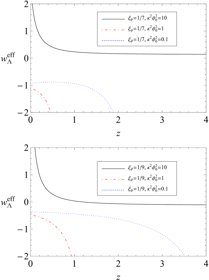
Figure 1: $w_{\rm\Lambda}^{eff}$ vs $z$ in the interacting canonical field case, for $\xi_{\phi}=1/7$, $\xi_{\phi}=1/9$, $b^{2}=0.01$ and $k=+1,0$, where in each case the combination $\kappa^{2}\phi_{0}^{2}$ is taken equal to $10$, $1$, $0.1$ respectively. The curves for $k=+1,0$ appear superimposed showing that the effect of the non-flat universe is negligible. The divergence of $w_{\rm\Lambda}^{eff}$ is a direct consequence of the singularity of (31), and thus the corresponding combinations of and $\kappa^{2}\phi_{0}^{2}$ must be excluded.

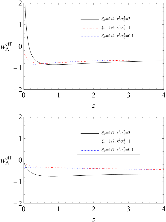
Figure 2: $w_{\rm\Lambda}^{eff}$ vs $z$ in the interacting phantom field case, for $\xi_{\sigma}=1/4$, $\xi_{\sigma}=1/7$, $b^{2}=0.01$ and $k=+1,0$, where in each case the combination $\kappa^{2}\sigma_{0}^{2}$ is taken equal to $3$, $1$, $0.1$ respectively. The curves for $k=+1,0$ appear superimposed showing that the effect of the non-flat universe is negligible. The divergence of $w_{\rm\Lambda}^{eff}$ is a direct consequence of the singularity of (48), and thus the corresponding combinations of and $\kappa^{2}\sigma_{0}^{2}$ must be excluded.

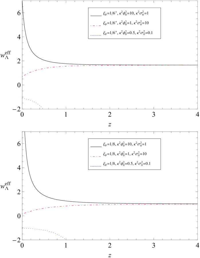
Figure 3: $w_{\rm\Lambda}^{eff}$ vs $z$ in the combined interacting quintom scenario, for $\xi_{\phi}=1/6^{+}$, $\xi_{\phi}=1/8$, $b^{2}=0.01$ and $k=+1,0$, where in each case the combinations $\kappa^{2}\phi_{0}^{2}$ and $\kappa^{2}\sigma_{0}^{2}$ are shown in the insets. The curves for $k=+1,0$ appear superimposed showing that the effect of the non-flat universe is negligible. The divergence of $w_{\rm\Lambda}^{eff}$ is a direct consequence of the singularity of (63), and thus the corresponding combinations of $\xi_{\phi}$, $\kappa^{2}\phi_{0}^{2}$ and $\kappa^{2}\sigma_{0}^{2}$ must be excluded.

4 Conclusions

Currently scalar fields play crucial roles in modern cosmology. In the inflationary scenario they generate an exponential rate of evolution of the universe as well as density fluctuations due to the vacuum energy. It seems that the presence of a non-minimal coupling (NMC) between scalar field and gravity is also necessary. There are many theoretical evidences that suggest the incorporation of an explicit NMC between the scalar field and gravity in the action [33]. The NMC arises from quantum corrections and it is required also by the renormalization of the corresponding field theory. Amazingly, it has been proven that the phantom divide line crossing of dark energy described by a single minimally coupled scalar field with general Lagrangian is even unstable with respect to the cosmological perturbations realized on the trajectories of the zero measure [34]. This fact has motivated a lot of attempts to realize the crossing of the phantom divide line by a equation of state parameter of the scalar field used as dark energy candidate in more complicated frameworks.
Studying the interaction between dark energy and ordinary matter will open the possibility of detecting dark energy. It should be pointed out that evidence was recently provided by the Abell Cluster A586 in support of the interaction between dark energy and dark matter [35]. However, despite the fact that numerous works have been carried out, at present there are no stringent observational bounds on the strength of this interaction [36]. This weakness to set stringent (observational or theoretical) constraints on the strength of the coupling between dark energy and dark matter stems from our unawareness of the nature and origin of the dark components of the Universe. It is therefore more than obvious that further work is needed in this direction. Due to this, we have extended our work in [26] to the interacting case in this paper. As a result, in the present paper we have investigated canonical, phantom and quintom models, with the various fields being non-minimally coupled to gravity, in the framework of the interacting HDE in non-flat universe. For this case, the characteristic length is no more the radius of the event horizon ($R_{E}$) but the event horizon radius as measured from the sphere of the horizon ($L$). In each case we have extracted $w_{\rm\Lambda}^{eff}$, that is, the dark energy effective equation of state parameter, as a function of the redshift and used as parameters the couplings and the amplitudes of the fields. Finally, we have analyzed it in order to obtain its cosmological implications.

5 Acknowledgment

The work of M. R. Setare has been supported by Research Institute for Astronomy and Astrophysics of Maragha, Iran. The work of Alberto Rozas-Fernández was supported by DGICYT (Spain) under Research Project No. FIS2005-01180.

References

• [1] S. Perlmutter et al, Nature (London), 391, 51, (1998); Knop. R et al., Astroph. J., 598, 102 (2003); A. G. Riess et al., Astrophy. J., 607, 665(2004); H. Jassal, J. Bagla and T. Padmanabhan, Phys. Rev. D, 72, 103503 (2005).
• [2] S.Nojiri and S. D. Odintsov, Phys. Rev. D 68, 123512 (2003); S.Nojiri and S. D. Odintsov, Int. J. Geom. Meth. Mod. Phys. 4, 115 (2007); M. R. Setare and E. N. Saridakis, Phys. Lett.  B 670, 1 (2008) [arXiv:0810.3296 [hep-th]].
• [3] B. Ratra and P. J. E. Peebles, Phys. Rev. D 37, 3406 (1988); C. Wetterich, Nucl. Phys. B 302, 668 (1988); A. R. Liddle and R. J. Scherrer, Phys. Rev. D 59, 023509 (1999) [arXiv:astro-ph/9809272]; I. Zlatev, L. M. Wang and P. J. Steinhardt, Phys. Rev. Lett. 82, 896 (1999); Z. K. Guo, N. Ohta and Y. Z. Zhang, Mod. Phys. Lett.  A 22, 883 (2007).
• [4] R. R. Caldwell, Phys. Lett. B 545, 23 (2002); R. R. Caldwell, M. Kamionkowski and N. N. Weinberg, Phys. Rev. Lett. 91, 071301 (2003); S. Nojiri and S. D. Odintsov, Phys. Lett. B 562, 147 (2003) [arXiv:hep-th/0303117]; V. K. Onemli and R. P. Woodard, Phys. Rev. D 70, 107301 (2004) [arXiv:gr-qc/0406098]; M. R. Setare, Eur. Phys. J. C 50, 991 (2007).
• [5] B. Feng, X. L. Wang and X. M. Zhang, Phys. Lett.  B 607, 35 (2005); Z. K. Guo, et al., Phys. Lett. B 608, 177 (2005); M.-Z Li, B. Feng, X.-M Zhang, JCAP, 0512, 002 (2005); B. Feng, M. Li, Y.-S. Piao and X. Zhang, Phys. Lett. B 634, 101 (2006); M. R. Setare, Phys. Lett. B 641, 130 (2006); W. Zhao and Y. Zhang, Phys. Rev. D 73, 123509 (2006); M. R. Setare, J. Sadeghi, and A. R. Amani, Phys. Lett. B 660, 299 (2008); J. Sadeghi, M. R. Setare, A. Banijamali and F. Milani, Phys. Lett. B 662, 92 (2008); M. R. Setare and E. N. Saridakis, Phys. Lett.  B 668, 177 (2008); M. R. Setare and E. N. Saridakis, [arXiv:0807.3807 [hep-th]]; M. R. Setare and E. N. Saridakis, JCAP 0809, 026 (2008).
• [6] E. Witten, hep-ph/0002297.
• [7] A. G. Cohen, D. B. Kaplan and A. E. Nelson, Phys. Rev. Lett.  82, 4971 (1999); P. Horava and D. Minic, Phys. Rev. Lett.  85, 1610 (2000); S. D. Thomas, Phys. Rev. Lett.  89, 081301 (2002).
• [8] S. D. H. Hsu, Phys. Lett. B 594, 13 (2004).
• [9] M. Li, Phys. Lett. B 603, 1 (2004); D. Pavon and W. Zimdahl, Phys. Lett. B 628, 206 (2005).
• [10] K. Enqvist and M. S. Sloth, Phys. Rev. Lett.  93, 221302 (2004); K. Ke and M. Li, Phys. Lett. B 606, 173 (2005); Q. G. Huang and M. Li, JCAP 0503, 001 (2005); E. Elizalde, S. Nojiri, S. D. Odintsov and P. Wang, Phys. Rev. D 71, 103504 (2005); B. Wang, Y. Gong and E. Abdalla, Phys. Lett. B 624, 141 (2005); S. Nojiri and S. D. Odintsov, Gen. Rel. Grav. 38, 1285 (2006); H. Kim, H. W. Lee and Y. S. Myung, Phys. Lett. B 632, 605 (2006); B. Hu and Y. Ling, Phys. Rev. D 73, 123510 (2006); H. Li, Z. K. Guo and Y. Z. Zhang, Int. J. Mod. Phys. D 15, 869 (2006); M. R. Setare, Phys. Lett. B 642, 421 (2006); M. R. Setare, Phys. Lett. B 644, 99 (2007); M. R. Setare, J. Zhang and X. Zhang, JCAP 0703 007 (2007); M. R. Setare, Phys. Lett. B 648, 329 (2007); M. R. Setare, Phys. Lett. B 654, 1 (2007); W. Zhao, Phys. Lett. B 655, 97, (2007); M. Li, C. Lin and Y. Wang, JCAP 0805, 023 (2008).
• [11] Q. G. Huang and Y. G. Gong, JCAP 0408, 006 (2004) [arXiv:astro-ph/0403590].
• [12] K. Enqvist, S. Hannestad and M. S. Sloth, JCAP 0502, 004 (2005) [astro-ph/0409275];
J. y. Shen, B. Wang, E. Abdalla and R. K. Su, Phys. Lett.  B 609, 200 (2005) [arXiv:hep-th/0412227].
• [13] Q. G. Huang and M. Li, JCAP 0503, 001 (2005) [arXiv:hep-th/0410095].
• [14] Q. G. Huang and M. Li, JCAP 0408, 013 (2004) [astro-ph/0404229].
• [15] P. Brax and J. Martin, JCAP 0611 (2006) 008 [arXiv:astro-ph/0606306].
• [16] W. Zimdahl and D. Pavon, Phys. Lett.  B 521 (2001) 133 [arXiv:astro-ph/0105479]; L. P. Chimento, A. S. Jakubi, D. Pavon and W. Zimdahl, Phys. Rev.  D 67 (2003) 083513 [arXiv:astro-ph/0303145]; S. del Campo, R. Herrera and D. Pavon, Phys. Rev.  D 70 (2004) 043540 [arXiv:astro-ph/0407047]; D. Pavon and W. Zimdahl, Phys. Lett.  B 628 (2005) 206 [arXiv:gr-qc/0505020].
• [17] L. Amendola and D. Tocchini-Valentini, Phys. Rev.  D 64 (2001) 043509 [arXiv:astro-ph/0011243].
• [18] B. Wang, J. Zang, C. Y. Lin, E. Abdalla and S. Micheletti, Nucl. Phys.  B 778 (2007) 69 [arXiv:astro-ph/0607126].
• [19] B. Wang, Y. g. Gong and E. Abdalla, Phys. Lett.  B 624 (2005) 141 [arXiv:hep-th/0506069].
• [20] O. Bertolami, F. Gil Pedro and M. Le Delliou, Phys. Lett.  B 654 (2007) 165 [arXiv:astro-ph/0703462].
• [21] M. Kesden and M. Kamionkowski, Phys. Rev. Lett.  97 (2006) 131303 [arXiv:astro-ph/0606566]; M. Kesden and M. Kamionkowski, Phys. Rev.  D 74 (2006) 083007 [arXiv:astro-ph/0608095].
• [22] S. Das, P. S. Corasaniti and J. Khoury, Phys. Rev.  D 73 (2006) 083509 [arXiv:astro-ph/0510628].
• [23] B. Wang, C. Y. Lin, D. Pavon and E. Abdalla, Phys. Lett.  B 662 (2008) 1 [arXiv:0711.2214 [hep-th]].
• [24] D. Pavon and B. Wang, Gen. Rel. Grav.  41 (2009) 1 [arXiv:0712.0565 [gr-qc]].
• [25] W. Zimdahl, Int. J. Mod. Phys.  D 17, 651 (2008) [arXiv:0705.2131 [gr-qc]].
• [26] M. R. Setare, E. N. Saridakis, Phys. Lett. B 671, 331, (2009).
• [27] M. Ito, Europhys. Lett. 71, 712 (2005).
• [28] H. Kim, H. W. Lee and Y. S. Myung, Phys. Lett. B 632, 605, (2006).
• [29] C. L. Bennett et al., Astrophys. J. Suppl. 148, 1 (2003); D. N. Spergel, Astrophys. J. Suppl. 148, 175, (2003).
• [30] M. Tegmark et al., astro-ph/0310723.
• [31] B. Wang, Y. Gong, and E. Abdalla, Phys. Lett. B 624, 141 (2005).
• [32] Kyong Hee Kim, Hyong Won Lee and Yun Soo Myung, Phys. Lett. B 648, 107 (2007).
• [33] V. Faraoni, Phys. Rev. D 53 (1996) 6813; V. Faraoni, Phys. Rev. D 62 (2000) 023504.
• [34] A. Vikman, Phys. Rev. D 71 (2005) 023515, [arXiv:astro-ph/0407107]; V. Sahni and Y. Shtanov, JCAP 0311 (2003) 014; F. Piazza and S. Tsujikawa, JCAP 0407 (2004) 004.
• [35] O. Bertolami, F. Gil Pedro and M. Le Delliou, Phys. Lett. B 654, 165 (2007) [arXiv:astro-ph/0703462]; M. Le Delliou, O. Bertolami and F. Gil Pedro, AIP Conf. Proc. 957, 421 (2007) [arXiv:0709.2505 [astro-ph]].
• [36] C. Feng, B. Wang, Y. Gong and R. K. Su, JCAP 0709, 005 (2007) [arXiv:0706.4033 [astro-ph]]; E. Abdalla, L. R. W. Abramo, L. . J. Sodre and B. Wang, ”Signature of the interaction between dark energy and dark matter in galaxy clusters,” arXiv:0710.1198 [astro-ph].