Perturbation theory for ac-driven interfaces in random media

Abstract

We study $D$-dimensional elastic manifolds driven by ac-forces in a disordered environment using a perturbation expansion in the disorder strength and the mean-field approximation. We find, that for $D\leq 4$ perturbation theory produces non-regular terms that grow unboundedly in time. The origin of these non-regular terms is explained. By using a graphical representation we argue that the perturbation expansion is regular to all orders for $D>4$. Moreover, for the corresponding mean-field problem we prove that ill-behaved diagrams can be resummed in a way, that their unbounded parts mutually cancel. Our analytical results are supported by numerical investigations. Furthermore, we conjecture the scaling of the Fourier coefficients of the mean velocity with the amplitude of the driving force $h$.

I Introduction

The theoretical analysis of pinning phenomena of elastic objects in random potentials is an important physical problem with a great impact on many fields of research Kardar (1998); Fisher (1998). Elastic objects in disordered media subject to a constant driving force are meanwhile well understood Brazovskii and Nattermann (2004) at zero temperature and the influence of finite temperature has been studied as well Chauve et al. (2000).

In recent years, also the problem of ac-driven elastic interfaces in disordered systems has gained experimental interest Kleemann et al. (2007); Kleemann (2007); Jeżewski et al. (2008). In experiments, considerable attention is devoted to the behaviour of the ac-susceptibility of ferroelectric thin films or ultrathin ferromagnetic multilayers, which is believed to be related to the motion of domain walls in these systems. So, an interest to understand ac-driven domain wall motion in disordered systems emerged. First results towards an explanation of the hysteretic behaviour of the magnetisation Lyuksyutov et al. (1999); Nattermann et al. (2001) have been achieved and the observed frequency regimes for the response of ferroic domain wall motion are understood phenomenologically Fedorenko et al. (2004). An important contribution comes from the velocity hysteresis of moving domain walls Glatz et al. (2003), but the characterising parameters have not yet been worked out. Generally, with regard to an analytic description of the domain wall motion characteristics, results are scarce. Yet, mainly numerical results have been obtained to describe qualitative features of such systems, like the hysteresis or double-hysteresis of the velocity Glatz et al. (2003); Glatz (2004); Petracic et al. (2004).

In many cases, for a first quantitative analysis of complicated non-linear problems one uses a perturbation expansion. However, perturbative approaches are sometimes hampered by mathematical subtleties, like non-analyticities or singular perturbation theory (cf. Bender and Orszag (1978)), or by physical obstacles such as non-perturbative excitations or strong coupling. The difficulty with perturbation theory as a tool for the analysis of pinned elastic objects has its own interesting history.

Until the beginning of the eighties, the lower critical dimension $d_{l}$ of the random field Ising model has been the subject of a long-lasting debate. Dimensional reduction predicted that the lower critical dimension equals $d_{l}=3$, whereas domain-wall arguments Imry and Ma (1975) lead to the conclusion, that $d_{l}=2$. Eventually, in 1984 a final decision could be made and dimensional reduction was proven to fail Imbrie (1984, 1985). The reason for the failure has been found later Fisher (1986); Villain (1988) to be connected with the existence of many metastable states for the domain walls separating different regimes in a multidomain configuration. The plethora of metastable states arises from the dominance of the disorder over the domain wall elasticity on length scales above the so-called Larkin length $L_{\text{p}}$ Larkin (1970) for sample dimensions $d<5$. A perturbative iteration to find the energy minimum will not necessarily yield the correct extremal state Villain and Séméria (1983); Engel (1985). Put in more mathematical terms, the formal perturbative treatment of the domain walls assumes an analytic disorder correlator. However, a functional renormalisation group (FRG) treatment shows Fisher (1986), that any initially analytic disorder correlator develops a cusp-singularity at a finite length scale, which is the Larkin length $L_{\text{p}}$.

This insight has important consequences for the problem of an interface in a disordered environment exposed to a constant driving force $h$. At zero temperature and for small external force $h$, the interface adjusts its configuration to balance the driving and the disorder, but remains pinned and does not move on large time scales. If $h$ is tuned to exceed a critical threshold $h_{\text{p}}$, then after transience has relaxed, the interface slides with a mean velocity $v$ that behaves as $v\sim(h-h_{\text{p}})^{\beta}$ for $h\searrow h_{\text{p}}$. The system undergoes a non-equilibrium phase transition, the so-called depinning transition, for which $v$ plays the role of an order parameter. The critical behaviour close to the depinning transition has been investigated in a number of works Nattermann et al. (1992); Narayan and Fisher (1992, 1993); Ertas and Kardar (1994); Leschhorn et al. (1997); Chauve et al. (2001); Le Doussal et al. (2002, 2004). Furthermore, the influence of finite temperature on this transition has been considered in several articles Chauve et al. (2000); Bustingorry et al. (2008); Kolton et al. (2009a). Even the scaling behaviour for small frequencies $\omega$ of an ac-drive on approaching the critical point $(h,\omega)=(h_{\text{p}},0)$ has been worked out Glatz et al. (2003).

The depinning transition can, however, not be accounted for by perturbatively expanding the disorder. Therefore, perturbation theory is not applicable for small constant driving forces.

To achieve deeper quantitative insight into the ac-dynamics of interfaces, perturbation theory seems to be the only feasible method. Clearly, in the vicinity of the critical point $(h,\omega)=(h_{\text{p}},0)$ perturbation theory is expected to yield erroneous results, if not properly combined with an FRG treatment. Yet, FRG equations for the similar problem of a constant driving force, have been obtained by the construction of a perturbative series and a subsequent $\epsilon$-expansion. So, understanding the perturbation theory is the first necessary starting point. As has been said, pure perturbative calculations are restricted to parameter regimes far away from the neighbourhood of the depinning transition. Thus, for sufficiently large frequencies and driving field amplitudes, from the physical point of view there appears to be no contraindication against a perturbative procedure. However, as will become clear in this article, for systems subject to periodic driving forces perturbation theory in the disorder strength gives non-regular contributions to the velocity corrections for an internal interface dimension $D\leq 4$. With the attribute non-regular we refer to expressions that grow unboundedly in time. Such unbounded contributions certainly do not reflect the true physical behaviour, but their origin deserves careful investigation. Far away from the critical point, this behaviour of perturbation theory cannot be related to the assumption of an analytic disorder correlator. Quite the contrary, working with a cusped disorder correlator brings additional difficulties due to the delta functions in its derivatives.

In section II, we introduce the equation of motion for ac-driven elastic manifolds in disordered media, and investigate its perturbative expansion. Although our model is taylored to describe elastic manifolds, like interfaces between two immiscible fluids or domain walls in ferroic systems, we believe that our analysis also covers a wide range of models for other interesting problems, e.g. charge density waves Grüner (1988) or flux lines in type-II superconductors Blatter et al. (1994); Giamarchi and Le Doussal (1994); Nattermann and Scheidl (2000). After analysing the first non-vanishing order, we derive the diagrammatic expansion to account for higher orders. This can be used to argue, that perturbation theory works for $D>4$. The failure of perturbation theory for $D\leq 4$ is then analysed and explained. The well-known suitability of perturbation theory for estimates of the velocity of domain walls driven by a constant force, far in the sliding regime, does not contradict our statements for the ac-driving. We are going to take a look at this as well. The technically involved and more mathematical treatments are taken out of the main text and given in the appendices B and C.

The failure of perturbation theory in all physically interesting cases $D\leq 4$ underlines the importance of the mean-field approach, which is the second central subject of this article. In section III, we explore the corresponding mean-field equation of motion and its perturbative expansion. After some illustration of the qualitative behaviour of the full solution, we prove, that the perturbative corrections are regular, i.e. they remain bounded in all orders. The bulk part of this inductive proof, the induction step, is outsourced to appendix E. Further, we show that for large enough driving field amplitudes, sufficiently strong elastic coupling and high frequencies, the perturbative results agree very well with the numerics for the full mean field equation of motion. We conclude our considerations of the mean-field problem by a numerical analysis of the lowest non-vanishing perturbative order, which yields the decay law of the Fourier coefficients with the driving field strength.

A table of frequently appearing symbols is provided in appendix F.

II The perturbative treatment of interfaces in disordered media

II.1 The model

Our analysis models interfaces and domain walls that are thin such that they can be described by elastic $D$-dimensional manifolds, embedded in a $D+1$ dimensional space. The manifold itself is parametrised by a $D$-dimensional set $x$ of coordinates and its position in space is given by $z(x,t)$. We confine ourselves to the study of the zero-temperature case, i.e. we do not take thermal noise into account. Moreover, our model assumes small gradients and does not allow for overhangs. We expose the interface to a periodic driving force

$$h(t)=h\cdot\cos\omega t.$$ (1)

Then, the overdamped dynamics of elastic interfaces can be described by the equation of motion

$$\gamma^{-1}\partial_{t}z(x,t)=\Gamma\nabla_{x}^{2}z+h(t)+u\cdot g(x,z),$$ (2)

which has already been introduced in earlier works Feigel’man (1983); Bruinsma and Aeppli (1984); Koplik and Levine (1985). In eq. (2), $\Gamma$ and $\gamma$ are the stiffness and the inverse mobility of the domain wall. For simplicity, we set $\gamma=1$ in the following. The function $g(x,z)$ describes the quenched disorder, taken to be Gaußian with the correlators given by

$$\left\langle g(x,z)\right\rangle = 0$$ (3)

$$\left\langle g(x,z)g(x^{\prime},z^{\prime})\right\rangle = \delta^{D}(x-x^{\prime})\Delta(z-z^{\prime}),$$ (4)

where $\left\langle\ldots\right\rangle$ denotes the average over disorder. The disorder correlator in $z$-direction is taken symmetric around 0 and decays exponentially on a length scale $\ell$. Further, we demand $\Delta(0)=1$, as the strength of the disorder shall be measured by $u$. To be definite, we choose

$$\Delta(z-z^{\prime})=\exp\left[-\left({z-z^{\prime}\over\ell}\right)^{2}\right]$$ (5)

in case we need a precise formula. This choice corresponds to the case of an elastic manifold exposed to random field disorder Leschhorn et al. (1997). Throughout the whole paper we assume weak disorder. This means, that pinning forces are weak and the interface is pinned at the fluctuations of the impurity concentration, and not at single pinning centres. A more precise definition can be found e.g. in Nattermann et al. (1990). For weak disorder, the random forces have to accumulate to overcome the elasticity. On small length scales, elastic forces dominate and the interface is essentially flat. By comparing the elastic and the disorder term in (2) one can estimate the length scale $L_{\text{p}}$, called the Larkin length, at which the two competing effects are of the same order. The result is

$$L_{\text{p}}=\left[{\Gamma\ell\over u}\right]^{2\over 4-D}.$$ (6)

Thus, the elastic term dominates on all length scales for $D>4$.

Finally, we specify the initial configuration for the equation of motion (2) to be a flat wall $z(x,t=0)\equiv 0$.

II.2 Perturbation theory - first order

The equation of motion (2) can only be solved via an expansion in the disorder strength $u$. We are going to derive the perturbation expansion directly for the equation of motion, since this appears simpler. There is, however, another approach via functional integrals which came in useful for the functional renormalisation group calculations in the case of a constant driving force. The reader who is more familiar with this technique may find a brief treatment in appendix A which reveals the connection to our methodology.

The expansion is naturally performed around the solution for the problem without disorder, i.e. where $u=0$. In this case, we have a flat wall following the driving field: $Z(t)=(h/\omega)\sin\omega t$. Thus, we decompose $z(x,t)$ into the disorder-free solution and a correction, i.e. $z(x,t)=Z(t)+\zeta(x,t)$. The equation of motion for the disorder correction $\zeta(x,t)$ is easily derived from eq. (2)

$$(\partial_{t}-\Gamma\nabla_{x}^{2})\zeta(x,t)=u\cdot g(x,Z+\zeta).$$ (7)

The Green function for the differential operator on the left hand side is the well-known heat kernel

$$(\partial_{t}-\Gamma\nabla_{x}^{2})G(x,t) = \delta^{D}(x)\delta(t)$$

$$G(x,t) = \Theta(t)\>\int{\text{d}^{D}k\over(2\pi)^{D}}\>\text{e}^{\text{i}kx-\Gamma k^{2}t}.$$ (8)

The $k$-integral has to be cut off at some scale $\Lambda$, corresponding to the inverse smallest length scale in the system. To set up the perturbation series, we expand the correction in the disorder strength

$$\zeta(x,t)=\sum\limits_{n=1}^{\infty}u^{n}\zeta_{n}(x,t)$$ (9)

and the disorder force around the non-disordered solution

$$g(x,Z+\zeta)=\sum\limits_{k=0}^{\infty}\partial^{k}_{2}g(x,Z){\zeta^{k}\over k!}.$$ (10)

Thus, we obtain an equation for the first order correction:

$$\zeta_{1}(x,t)=\int\text{d}^{D}x^{\prime}\int\limits_{0}^{\infty}\text{d}t^{\prime}\>G(x-x^{\prime},t-t^{\prime})g(x^{\prime},Z(t^{\prime})).$$ (11)

Obviously, the disorder average vanishes. The disorder average for the second order contribution is given by

$$\left\langle\zeta_{2}\right\rangle(t)= \int\limits_{0}^{t}\text{d}t_{1}\int\limits_{0}^{t_{1}}\text{d}t_{2}\>\Delta^{\prime}[Z(t_{1})-Z(t_{2})]\times$$

$$\int{\text{d}^{D}k\over(2\pi)^{D}}\>\text{e}^{-\Gamma k^{2}(t_{1}-t_{2})}.$$ (12)

The second order correction to the velocity follows straightforwardly

$$\left\langle v_{2}\right\rangle(t)= \int\limits_{0}^{t}\text{d}t^{\prime}\>\Delta^{\prime}[Z(t)-Z(t^{\prime})]\int{\text{d}^{D}k\over(2\pi)^{D}}\>\text{e}^{-\Gamma k^{2}(t-t^{\prime})}.$$ (13)

To get a first impression on how this expression behaves for large $t$, we split off the Fourier-0-mode:

$$\Delta^{\prime}[Z(t)-Z(t^{\prime})] =F_{0}(\omega t)/\ell+p(t,t^{\prime})$$ (14)

$$F_{0}(\omega t) =\sum\limits_{n=0}^{\infty}K_{n}\left({h\over\omega\ell}\right)\cdot\sin(2n+1)\omega t.$$ (15)

Here, $p(t,t^{\prime})$ is a well-behaved oscillation around 0 in $t^{\prime}$. Since $p(t,t^{\prime})$ yields a bounded contribution to $\left\langle v_{2}\right\rangle(t)$, we consider only $F_{0}(t)$ to find out, how $\left\langle v_{2}\right\rangle$ increases asymptotically in time. The Fourier coefficients $K_{n}$ can be determined analytically. They are diminished when their argument increases or approaches zero and they remain bounded. Integration over $t^{\prime}$ yields

$$\left\langle v_{2}\right\rangle(t) \sim{F_{0}(\omega t)\over\ell}{S_{D}\over(2\pi)^{D}}\int\limits_{0}^{\Lambda}{\text{d}k\over\Gamma}\>k^{D-3}\left[1-\text{e}^{-k^{2}\Gamma t}\right]$$ (16)

$$={t^{2-D\over 2}\over\ell}{F_{0}(\omega t)\over\Gamma^{D/2}}\cdot a_{D}(t/\vartheta),$$ (17)

where

$$a_{D}(x) ={S_{D}\over(2\pi)^{D}}\int\limits_{0}^{\sqrt{x}}\text{d}p\>p^{D-3}\left[1-\text{e}^{-p^{2}}\right].$$ (18)

For $x\to\infty$ the integral $a_{D}$ converges for $D<2$ and diverges logarithmically for $D=2$. Thus, the asymptotic behaviour of the first perturbative correction in time is given by

$$\left\langle v_{2}\right\rangle(t) \sim c_{D}(t)\cdot\left\{\begin{matrix}t^{2-D\over 2}&D<2\\ \log t&D=2\\ \text{const}&D>2\end{matrix}\right.$$ (19)

where $c_{D}(t)$ is some bounded function.

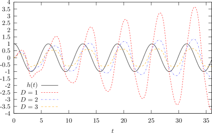
Figure 1: Plot of the first non-vanishing perturbative correction $\left\langle v_{2}\right\rangle(t)$ to the disorder average $\left\langle v(x,t)\right\rangle$ for different interface dimensions. For the plot we used $h=1$ and the units are chosen such that $\omega=\ell=1$.

Fig. 1 shows the plots of $\left\langle v_{2}\right\rangle(t)$ for $D=1,2,3$. Obviously, there is a problem of the perturbation expansion in low dimensions. In the following, we are going to see that perturbation theory does not work even for $D\leq 4$.

II.3 Higher order graphical expansion

Higher orders of the perturbation expansion are best expressed diagramatically. To deduce the diagrammatic rules, all one has to do is plugging (9) into (10), rearranging the sum in powers of $u$ and inserting this into (7). The diagrammatic rules that emerge are fairly simple: to express the perturbative correction of order $n$, we draw all rooted trees with $n$ vertices and add a stem. Up to the fourth order, this tree graph expansion is given by

$$\zeta_{1} =$$

$$\zeta_{2} =$$

$$\zeta_{3} = \parbox{48.36967pt}{\includegraphics{vzdiag3.eps}}\>+\>\parbox{71.13188pt}{\includegraphics{vzdiag4.eps}}$$

$$\zeta_{4} = \parbox{48.36967pt}{\includegraphics{vzdiag5.eps}}\>+\>\parbox{91.04881pt}{\includegraphics{vzdiag6.eps}}\>+$$ (23)

$$\parbox{71.13188pt}{\includegraphics{vzdiag7.eps}}\>+2\cdot\>\parbox{71.13188pt}{\includegraphics{vzdiag8.eps}}$$

Every vertex represents a disorder insertion $g^{(m)}(Z(t))/m!$, where $m$ counts the number of outgoing branches (away from the root). Every line corresponds to an integral operator, the kernel being the propagator $G(x,t)$. To get the graphical expansion for the velocities, just remove the first line. The disorder average can be carried out using Wick’s theorem, since our disorder is assumed to be Gaußian. An immediate consequence is, that after averaging over disorder, only graphs with an even number of vertices survive. In the following, we are going to consider the perturbation expansion for the disorder averaged velocity $v(t)$. The pairing for the disorder average shall be denoted by a dashed line. An example graph from the $4^{\text{th}}$-order is

$$\parbox{71.13188pt}{\includegraphics{exdiag1.eps}}.$$ (24)

Using this graphical expansion, in appendix B we take a look at the general behaviour of the diagrammatic contributions to all orders for $t\to\infty$ and argue that all graphs remain bounded in case $D>4$.

II.4 The failure of perturbation theory for $D\leq 4$

For $D\leq 4$ the perturbation expansion is not as well-behaved as for $D>4$. In this section, we show this and give an explanation why perturbation theory is ill-behaved in low dimensions.

Though the disorder averaged graphical structure can become complicated, one especially simple graph has the same structure in all orders: the one for which all vertices are connected directly to the root. In the equations (II.3-23), we have drawn those graphs at the very first place. Let us call them bushes. The general bush graph contribution to the velocity correction of order $2p$ thus corresponds to the following diagram

$$\left\langle B_{2p}\right\rangle =\>\parbox{36.98857pt}{\includegraphics{bdiaga.eps}},$$ (25)

where the dotted line is a placeholder for other vertices that we have not drawn. Up to combinatorical factors, the general (disorder averaged) bush $B_{2p}$ that occurs in the $2p$-th order perturbative correction to the velocity $v$, reads

$$\left\langle B_{2p}\right\rangle (t)\propto$$

$$\bigg{[}\int\limits_{0}^{t}\text{d}t_{1}\text{d}t_{2}\>\Delta[Z_{1}-Z_{2}]\int{\text{d}^{D}k\over(2\pi)^{D}}\>\text{e}^{-\Gamma k^{2}(2t-t_{1}-t_{2})}\bigg{]}^{p-1}$$

$$\times\int\limits_{0}^{t}\text{d}t^{\prime}\>\Delta^{(2p-1)}[Z-Z^{\prime}]\int{\text{d}^{D}k\over(2\pi)^{D}}\>\text{e}^{-\Gamma k^{2}(t-t^{\prime})}$$ (26)

$$\equiv T_{1}^{p-1}\cdot T_{2}$$ (27)

To work out the asymptotic envelope of $\left\langle B_{2p}\right\rangle(t)$ for large $t$ we only need to take a look at the expression $T_{1}$. Since $\Delta$ is an entirely positive function, and the $k$-integral is certainly non-negative, we can replace $\Delta$ by its maximum $\Delta(0)$ to get an upper bound, and if we replace $\Delta$ by the minimal value that is taken $\Delta[2h/(\omega\ell)]$, we get a lower bound for $T_{1}$. In both cases, $\Delta[Z(t_{1})-Z(t_{2})]$ is replaced by a constant, so that the integration over $t_{1}$ and $t_{2}$ can be done easily. Consequently, up to a constant, the asymptotic envelope of $T_{1}$ is given by

$${u^{2}\over\ell^{2}}T_{1}(t)\sim {u^{2}\over\ell^{2}}\int{\text{d}^{D}k\over(2\pi)^{D}}{\left[1-\text{e}^{-\Gamma k^{2}t}\right]^{2}\over\Gamma^{2}k^{4}}$$

$$= \left[{t\over\tau}\right]^{4-D\over 2}A_{D}(t/\vartheta).$$ (28)

Here, the constants $\tau$ and $\vartheta$ are time scales, given by

$$\tau =\Gamma^{D\over 4-D}\left[{\ell\over u}\right]^{4\over 4-D}=\left({\ell\over u}\right)L_{\text{p}}^{D\over 2}=L_{\text{p}}^{2}/\Gamma$$ (29)

$$\vartheta =\Lambda^{-2}/\Gamma$$ (30)

and the function $A_{D}(x)$ has been introduced for notational convenience

$$A_{D}(x)={S_{D}\over(2\pi)^{D}}\int\limits_{0}^{\sqrt{x}}\text{d}p\>p^{D-5}\left[1-\text{e}^{-p^{2}}\right]^{2}.$$ (31)

The function $A_{D}(x)$ is increasing but bounded for $D<4$ and grows logarithmically as $x\to\infty$ for $D=4$. Thus $T_{1}$ grows monotonically in $t$ for any $D\leq 4$.

Actually, our statement about the asymptotics in eq. (II.4) is more robust than our simple argument suggests, and in fact does not rely on the positivity of $\Delta$. A more detailed calculation, presented in appendix C shows that

$${u^{2}\over\ell^{2}}T_{1}= \left({t\over\tau}\right)^{4-D\over 2}\kappa_{D}\left({t\over\vartheta}\right)+$$

$$\left({t\over\tau}\right)^{4-D\over 4}{u\Lambda^{D\over 2}\over\omega\ell}k_{D}\left({t\over\vartheta},\omega t\right)+$$

$${u^{2}\Lambda^{D}\over\omega^{2}\ell^{2}}P_{D}\left({t\over\vartheta},\omega t\right)$$ (32)

and

$${u^{2}\ell^{2(p-1)}\over\omega\ell}T_{2}= {u\Lambda^{D\over 2}\over\omega\ell}\left({t\over\tau}\right)^{4-D\over 4}f_{D}\left({t\over\vartheta},\omega t\right)+$$

$${u^{2}\Lambda^{D}\over\omega^{2}\ell^{2}}p_{D}\left({t\over\vartheta},\omega t\right)$$ (33)

where all of the functions $\kappa_{D}$, $k_{D}$, $P_{D}$, $f_{D}$ and $p_{D}$ are bounded in $t$ for $D<4$. The first term of $T_{1}$ shows, that for $D\leq 4$ the whole expression grows for $t\to\infty$ without any bound. This is, because by definition (cf. equation (118)), $\kappa_{D}\propto A_{D}$, where $A_{D}$ is given by (31). The other tree graphs that appear in the graphical representation of $\left\langle v_{2p}\right\rangle$ and that we have not analysed here, exhibit similar behaviour. Cancellations among diagrams do not occur. To have a little more evidence, that $D=4$ really enters as an upper critical dimension, we have perturbatively investigated the interface’s width in appendix D. In summary, perturbation theory is ill behaved for $D\leq 4$. The reason for this shall be discussed in the following.

The bushes $\left\langle B_{2p}\right\rangle$ that we have considered so far are part of an expansion of the disorder averaged velocity

$$v(t)=h\cdot\cos\omega t+v_{\text{dis}}(t)$$ (34)

in the disorder strength $u$. The dimensionless ratios, in which $u$ occurs in that expansion are

$$\left({t\over\tau}\right)^{4-D\over 4}\quad\text{and}\quad{u\Lambda^{D\over 2}\over\omega\ell}.$$ (35)

Since in the stationary state the interface is expected to follow the driving with frequency $\omega$, its Fourier representation has to take on the form

$$v_{\text{dis}}(t)=\omega\ell\sum\limits_{n} e_{n}\left(\left({t\over\tau}\right)^{4-D\over 4},{u\Lambda^{D\over 2}\over\omega\ell},{t\over\vartheta}\right)\cos n\omega t+$$ (36)

$$f_{n}\left(\left({t\over\tau}\right)^{4-D\over 4},{u\Lambda^{D\over 2}\over\omega\ell},{t\over\vartheta}\right)\sin n\omega t.$$ (37)

Because of the ratio $t/\tau$, an expansion in the disorder $u$ brings powers of $t^{4-D\over 4}$ in every order, since $\tau$ depends on $u$ (cf. equation (29)). The remaining question is the meaning of $\tau$. Since $\tau$ appears as a time scale for the time dependence of the Fourier coefficients, which physically should approach a constant value in the stationary state $t\to\infty$, the most natural interpretation is the transience. Keeping in mind, that we start with a flat wall, we have to expect several kinds of transience effects. As we have seen, there are only two time scales in question: $\tau$ and $\vartheta$. As can be concluded from their definitions (cf. equations (29) and (30)), they obey the same structure: an intrinsic length scale to the power 2 divided by $\Gamma$. The time scale $\tau$ involves the Larkin length $L_{\text{p}}$ (cf. equation (6)), which measures the competition between disorder and elasticity: the interface is flat on length scales $L\lesssim L_{\text{p}}$. This indicates that, up to some dimensionless prefactor, $\tau$ describes the time during which correlated interface segments of extension $L_{\text{p}}$ adopt to their local disorder environment, i.e. the roughening time of the interface. For $D>4$, the interface is flat on all length scales, thus there is neither roughening nor a Larkin length, hence $\tau$ is meaningless and cannot occur. This agrees with our observation. For $D>4$, there is no disorder-dependent time scale any more, which could bring powers of time in the perturbative corrections, therefore they remain finite as $t\to\infty$. However, also for $D>4$ the disorder leads to a typical deviation of every point of the interface from the mean position. The built-up of this typical deviation towards its steady-state value happens on the time-scale $\vartheta$, in agreement with the observation for mean-field theory (cf. section III.3). Thus, both time scales can naturally be interpreted as the life times of two different transience effects.

II.5 Interfaces subject to a constant driving force

In the introduction, we already pointed out that perturbation theory in connection with interfaces driven by a constant force cannot properly account for the existence of the depinning transition and therefore gives misleading results for $D\leq 4$. But far above the depinning threshold, i.e. for $h\gg h_{\text{p}}$, the interface slides and its velocity can be estimated perturbatively. The dynamical correlation length $L_{v}=\Gamma\ell/v$ Leschhorn et al. (1997) is then small compared to the Larkin length $L_{\text{p}}$ and thus working with an analytic disorder correlator and expanding the disorder in its moments works. Of course, also for constant driving forces one has to start with a definite initial condition, which is usually a flat wall. Thus, there will be transience effects for dc-driven interfaces as well Schehr and Le Doussal (2005); Kolton et al. (2009b). In this section we take a short glance to understand the difference between ac and dc-driving. Our special interest is devoted to the time scales that determine the duration of transience effects.

The equation of motion for the elastic interface experiencing a constant driving force

$$\partial_{t}z(x,t)=\Gamma\nabla_{x}^{2}z+h+u\cdot g(x,z),$$ (38)

has the disorder-free solution ($u=0$) $Z(t)=ht$. The perturbation expansion is essentially the same as in section II.2, just the non-disorded solution around which we expand is different.

Actually, there is a problem with the decomposition $z=Z+\zeta$ here, since the sliding velocity $v$ is different from $h$, hence $\zeta\sim(v-h)t$ is not a small quantity (compared to $\ell$) for large $t$ and the Taylor expansion (10) of the disorder is questionable. Since here we shall not be interested in large times $t>\ell/(h-v)$ but only want to determine the time scale of the transience (occuring at small $t\ll\ell/(h-v)$), this problem is safely ignored.

The first non-vanishing correction to the velocity is found to be (cf. eq. (13))

$$\left\langle v_{2}\right\rangle(t)= \int\limits_{0}^{t}\text{d}t^{\prime}\>\Delta^{\prime}[Z(t)-Z(t^{\prime})]\int{\text{d}^{D}k\over(2\pi)^{D}}\>\text{e}^{-\Gamma k^{2}(t-t^{\prime})}$$ (39)

$$= {1\over h}\int{\text{d}^{D}k\over(2\pi)^{D}}\left[\text{e}^{-k^{2}\Gamma t-{h^{2}t^{2}\over\ell^{2}}}-\varphi\left({\Gamma\ell k^{2}\over 2h},{ht\over\ell}\right)\right]$$ (40)

$$= {\Lambda^{D}\over(t/\vartheta)^{D\over 2}h}{S_{D}\over(2\pi)^{D}}\int\limits_{0}^{\sqrt{t/\vartheta}}\text{d}p\>p^{D-1}\times$$

$$\left[\text{e}^{-p^{2}-{{h^{2}t^{2}\over\ell^{2}}}}-\varphi\left({p\over 2}{{\ell\over ht}},{{ht\over\ell}}\right)\right]$$ (41)

where we have introduced the function

$$\varphi(a,b)=1-\sqrt{\pi}\,a\cdot\text{e}^{a^{2}}\cdot\big{[}\text{erf}(a+b)-\text{erf}(a)\big{]}$$ (42)

for convenience. The time-scales on which transience effects disappear are obviously given by

$$\tau_{\text{dc}}={\ell\over h}={L_{h}^{2}\over\Gamma}\quad\text{and}\quad\vartheta={\Lambda^{-2}\over\Gamma}$$ (43)

and are manifestly disorder-independent. $L_{h}=\Gamma\ell/h$ denotes the correlation length of an interface moving with a velocity $h$. Of course, asymptotically the interface moves with a velocity $v<h$, but at the very beginning, when we start off with a flat wall, its velocity is indeed given by $h$ (cf. (38)).

It is not surprising, that the time scale of the initial roughening is different for dc and ac driving. Either problem involves completely different physical processes to be responsible for transience. In the case of an ac-driving, the system undergoes a process of adaption of its configuration to the local disorder, such that a stable stationary oscillation is possible, and during which higher Fourier modes build up. For dc-driving, the system starts to move with a velocity of $h$, which then rapidly decreases, and roughens since segments of the interface are pinned and remain at rest until they are pulled forward by the neighbouring segments through the elastic coupling. The time for this process mainly depends on the velocity of the interface, not on the strength of the disorder.

III Mean field theory

To extend the study of ac-driven interfaces beyond numerics, perturbation theory seems unavoidable. Since, as we have seen in the preceeding section, perturbation theory only works for $D>4$, we turn here to an interesting limiting case, formally corresponding to $D=\infty$: the mean-field equation of motion.

Mean field calculations have been performed before for the problem of interfaces and charge density waves subject to a constant driving in a number of articles Fisher (1983, 1985); Leschhorn (1992); Narayan and Fisher (1992); Lyuksyutov (1995). Special emphasis has been put on the depinning transition and its critical properties.

The perturbation expansion for dc-driven interfaces has been investigated by Koplik and Levine Koplik and Levine (1985), who also emphasised on the mean-field problem. They already mentioned the same problematic graphs in their expansion that we will encounter below, but they did not provide a proof for the fact, that the unbounded terms cancel to all orders, independent of the driving.

III.1 The mean-field equation of motion

The mean field equation corresponding to our original equation of motion (2) is obtained via the replacement of the elastic term by a uniform long-range coupling (cf. e.g. Fisher (1985)). To do this, we have to formulate the model (2) on a lattice in $x$-direction, i.e. the coordinates that parameterise the interface itself are discretised. The lattice Laplacian reads

$$\nabla_{x}^{2}z(x_{i}) =\sum\limits_{d=1}^{D}{z(x_{i}+ae_{d})+z(x_{i}-ae_{d})-2z(x_{i})\over a^{2}}$$

$$=\sum\limits_{d=1}^{D}\sum\limits_{j_{d}=1}^{N}J_{ij_{d}}\big{[}z(x_{j_{d}})-z(x_{i})\big{]},$$ (44)

$$J_{ij_{d}} ={1\over a^{2}}\big{[}\delta_{j_{d}+1,i}+\delta_{j_{d}-1,i}\big{]},$$ (45)

where $a$ denotes the lattice constant. To get the mean field theory, $J_{ij}$ has to be replaced by a uniform coupling but such that the sum over all couplings $\sum_{j}J_{ij}$ remains the same. Hence, we choose

$$J_{ij}^{\rm MF}={1\over a^{2}N}.$$ (46)

Now, the disorder has to be discretised as well, which is achieved if we replace the delta function in the correlator (4) by $\delta^{D}(x_{i}-x_{j})\to\delta_{ij}a^{-D/2}$ (cf. Bruinsma and Aeppli (1984)). The resulting equation of motion should be independent of $x$, just the lattice constant $a$ and the dimension enter because the disorder scales with a factor $a^{-D/2}$. Finally, for the mean-field equation of motion, we obtain

$$\partial_{t}z =c\cdot\left[\left\langle z\right\rangle-z\right]+h(t)+\eta\cdot g(z),$$ (47)

where $c=\Gamma/a^{2}$ and $\eta=u/a^{D/2}$. The disorder remains Gaußian with

$$\left\langle g(z)\right\rangle = 0$$ (48)

$$\left\langle g(z)g(z^{\prime})\right\rangle = \Delta(z-z^{\prime}).$$ (49)

The function $\Delta(z-z^{\prime})$ is as before, so we shall choose again (5) whenever we need an explicit expression for calculations.

The physical picture of the mean field equation of motion is a system of distinct particles, moving in certain realisations of the disorder. All of them are harmonically coupled to their common mean, i.e. the elastic coupling between neighbouring wall segments $\Gamma\nabla_{x}^{2}z$ is now replaced by a uniform coupling $c\cdot\left[\left\langle z\right\rangle-z\right]$ to the disorder averaged position $\left\langle z\right\rangle$, which in turn is determined self-consistently by the single realisations.

Apart from the correlation length $\ell$ of the disorder, there is another important length scale in the system. In the absence of any driving force (i.e. $h=0$), we can easily determine the mean deviation of the coordinate $z$ of a special realisation from the disorder averaged position $\left\langle z\right\rangle$. For $h=0$ we expect $\dot{z}=0$, at least in the steady state and (47) straightforwardly leads to

$$\left\langle(\left\langle z\right\rangle-z)^{2}\right\rangle\simeq{\eta^{2}\over c^{2}}.$$ (50)

So, $\eta/c$ measures the order of the average distance from the common mean.

In what follows, the disorder averaged velocity $v=\left\langle\dot{z}\right\rangle$ will be denoted by the symbol $v$.

III.2 Qualitative behaviour and numerical results

To get an idea about how the system, corresponding to the equation of motion with an ac-driving (cf. (47))

$$h(t)=h\cdot\cos\omega t$$ (51)

behaves, we implemented a numerical approach. The disorder is modelled by concatenated straight lines, the values of the junction points are chosen randomly from a bounded interval. The correlator has been checked to be perfectly in agreement with (5).

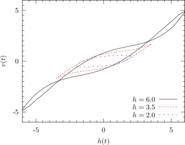
Figure 2: Numerical solution of (47) for different driving field strengths and $c=1.0$, $\eta=2.5$. For the simulation, $t$ and $z$ are measured in units such that $\omega=\ell=1$.

Before discussing the numerical trajectories, we note a first property of the equation of motion (47). It contains a symmetry of the (disorder averaged) system, namely that all disorder averaged quantities are invariant under the transformation $h\to-h$ and $z\to-z$, which implies $v\to-v$. We have hereby fixed the initial condition to be $z(0)=0$ for all realisations. If one chooses another initial condition, its sign has to be inverted as well, of course. In the steady state, i.e. for $t\gg c^{-1}$ (as $c^{-1}$ is the time-scale on which transience effects are diminished, see below), the trajectory must therefore obey the symmetry $h\to-h$, $v\to-v$. This symmetry is obviously reflected in the numerical solutions (see fig. 2).

An interesting consequence of this symmetry is, that the even Fourier coefficients of the solution $v(t)$ (which is periodic with period $2\pi/\omega$) vanish. Once the steady state is reached, the symmetry requires $v(t)=-v(t+\pi/\omega)$. For the even Fourier modes this means

$$c_{2N} =\int\limits_{0}^{2\pi\over\omega}\text{d}t\>v(t)\text{e}^{\text{i}2N\omega t}$$

$$=\int\limits_{0}^{\pi\over\omega}\text{d}t\>v(t)\text{e}^{\text{i}2N\omega t}+\int\limits_{0}^{\pi\over\omega}\text{d}t\>v\left(t+{\pi\over\omega}\right)\text{e}^{\text{i}2N\omega t}=0.$$ (52)

The typical picture of a $v$-$h$-plot is that of a single hysteresis for $h\ll\eta$ and a double hysteresis for $h\gg\eta$. In an intermediate range, we find a single hysteresis with a cusped endpoint. The qualitative shape of the solution trajectories, examples of which are shown in fig. 2, agrees with numerical results Glatz et al. (2003); Glatz (2004), that have been obtained as solutions for (2) in the case of finite interfaces with periodic boundary conditions.

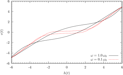
Figure 3: Numerical solution of equation (47) for $h=6.0$, $c=1.0$ and $\eta=2.5$ for different frequencies, $t$ and $z$ being measured in units such that $\omega_{0}=\ell=1$.

Moreover, as the frequency is sent to zero $\omega\to 0$, the hysteretic trajectory approaches the depinning curve for an adiabatic change of the driving field. This is shown in fig. 3.

In the following, we want to give a qualitative discussion of the hystereses in the case of small elasticity $c$, more precisely our discussion assumes $\eta/c\gg\ell$.

Weak fields $h\ll\eta$: For each disorder realisation, the configuration is allowed to deviate from the mean by an order of $\eta/c$ (cf. (50)), which by our assumption is large compared to the disorder correlation length $\ell$. So, except for rare events, in the case of weak driving fields, the typical system in a certain disorder configuration remains in a potential well of the disorder. Starting at some large time $t_{0}$ (in the steady state) for which $h(t_{0})=0$, we expect a certain realisation to be located close to a zero point $z_{0}$ of a falling edge of the disorder force $g(z_{0})=0$, since this corresponds to a stable configuration. As the field grows, the system starts to move in the direction of growing $z$, where the disorder force competes with the driving. Because in the vicinity of the potential minimum, the disorder force $g(z)$ behaves approximately linear in $z$, the acceleration is approximately zero and the velocity almost constant. This changes when the driving is about to reaching its maximum. The slower the growth of the driving, the smaller the velocity. At the maximum, the velocity equals zero, as the driving and the restitutional disorder force compensate. For decreasing $h(t)$, the restitution force wins and pushes the system back in the direction of the potential minimum. Hence, the velocity $v$ turns negative short-time after the field has reached its maximum and is still positive. Once the stable position $z_{0}$ is reached again, the same starts in the negative direction.

Certainly, the restitutional disorder force need not continuously grow with $z$, but may exhibit bumps or similar noisy structure, but those details average out when taking the mean over all disorder configurations.

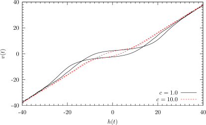
Figure 4: Numerical solution of equation (47) for different elastic constants and $h=40.0$, $\eta=10.0$. The units of $t$ and $z$ are chosen such that $\omega=\ell=1$.

Strong fields $h\gg\eta$: In the case of strong driving amplitudes, we encounter the situation of a double hysteresis. Again, starting at a time $t_{0}$ with $h(t_{0})=0$ for $t_{0}\gg c^{-1}$, we may assume the system to be located close to a zero $g(z_{0})=0$ of a falling edge of the disorder force field. As $h(t)$ grows, we first have the same situation as in the case of weak driving: The disorder acts restitutionally and thus keeps the velocity small and leads to a small slope $\text{d}v/\text{d}h$. Once the field is of the order $\eta$, the system is no longer locked into a potential well, but a cross-over to sliding behaviour sets in. On further increasing $h$, the system finally arrives at a slope $s=\text{d}v/\text{d}h$, which depends mainly on $\eta$ and $h$. The larger $h$, the closer $s$ approaches the value of 1. After the field reaches its maximum, the velocity decreases with the field, the slope being smaller than $s$, if $h$ is not too large. This is explained as follows. The mean deviation $\left\langle(\left\langle z\right\rangle-z)^{2}\right\rangle$ that we have estimated to be of the order $\eta^{2}/c^{2}$ for $h=0$ (cf. eq. (50)), under driving also depends on the difference between $v(t)$ and $h(t)$ (as can be seen from (47)). At the beginning of the crossover to sliding, when $h\approx\eta$, this difference is large and therefore also the mean deviation is large (especially for small $c$). When $h$ increases, the particles in disorder realisations that are behind the mean are strongly accelerated. On the other hand, those that are ahead of the mean position are not so much decelerated, because for each disorder realisation, being ahead of or behind the mean position rapidly changes and a motion backwards (against the driving) is suppressed. Thus the reduction of the mean deviation towards some asymptotic value gives a stronger slope for rising fields during the crossover. When the field $h(t)$ reduces, the mean deviation shrinks, $h(t)$ approaching $v$, and $v$ drops less rapidly than it has risen because still the mean deviation prefers a diminution of the difference $v(t)-h(t)$. This approximately linear reduction of the velocity remains, until the field is weaker than the typical disorder force, when the system is again trapped in a potential well. Since on rising edges of the disorder force, driving and disorder point in the same direction, the system will rarely sit there (it moves away very fast). The velocity becomes negative before $h=0$, since the system slides down the falling edge ($\text{d}g/\text{d}z<0$) of the disorder force. At $h=0$ everything starts again in the negative direction. An example for fairly large field amplitudes is shown in fig. 4.

So far, our discussion has emphasised on small $c$. The effect of larger $c$ is to couple the configuration $z(t)$ of every realisation strongly to the mean $\left\langle z(t)\right\rangle$. This wipes out the effect of disorder. Thus for larger $c$ the double hysteresis winds around a straight line, connecting the extremal velocities. This can be seen in fig. 4.

III.3 Mean-field perturbation theory

III.3.1 The diagrammatic expansion

Since the mean-field equation of motion (47) cannot be solved exactly, we attempt an expansion in the disorder strength $\eta$. Therefore, as before, we decompose $z=Z+\zeta$, where $Z(t)=(h/\omega)\sin\omega t$ is the solution of the non-disordered problem ($\eta=0$) around which we expand, and

$$\zeta=\sum\limits_{k=1}^{\infty}\zeta_{k}\eta^{k}\>,\quad\left\langle\zeta\right\rangle=\sum\limits_{k=1}^{\infty}\left\langle\zeta\right\rangle_{k}\eta^{k}.$$ (53)

is the perturbative correction. Still, we have the equations for $\zeta_{k}$ depending on $\left\langle\zeta\right\rangle_{k}$, which is also unknown. This eventually leads us to a set of two coupled equations

$$(\partial_{t}+c)\zeta =c\left\langle\zeta\right\rangle+\eta\cdot g(Z+\zeta)$$ (54)

$$\partial_{t}\left\langle\zeta\right\rangle =\eta\cdot\left\langle g(Z+\zeta)\right\rangle,$$ (55)

that we can solve iteratively for every order of the perturbation series, if we expand

$$g(Z+\zeta)=\sum\limits_{n=0}^{\infty}{g^{(n)}(Z)\over n!}\zeta^{n}.$$ (56)

If one is interested to keep small orders, this expansion of the disorder can only work if $\zeta\ll\ell$, because $\ell$ is the typical scale on which $g(z)$ changes. We will come back to that point later in section III.3.3, when discussing the validity of perturbation theory. For the moment, we just do it.

The propagator corresponding to the left hand side of Eq. (54) reads

$$G(t)=\Theta(t)\cdot\text{e}^{-ct}.$$ (57)

Using this propagator, we can formally write down the solution and express it order by order in a power series in $\eta$. Up to the second order, the solutions are

$$\left\langle\zeta\right\rangle_{1}(t) =0,$$ (58)

$$\zeta_{1}(t) =\int\limits_{0}^{t}\text{d}t_{1}\>\text{e}^{-c(t-t_{1})}g(Z(t_{1})),$$ (59)

$$\left\langle\zeta\right\rangle_{2}(t) =\int\limits_{0}^{t}\text{d}t_{1}\int\limits_{0}^{t_{1}}\text{d}t_{2}\>\text{e}^{-c(t_{1}-t_{2})}\Delta^{\prime}[Z(t_{1})-Z(t_{2})],$$ (60)

$$\zeta_{2}(t) =\int\limits_{0}^{t}\text{d}t_{1}\text{e}^{-c(t-t_{1})}\left[c\left\langle\zeta\right\rangle_{2}(t_{1})+g^{\prime}(Z(t_{1}))\cdot\zeta_{1}(t_{1})\right].$$ (61)

Since we assume Gaußian disorder, the disorder averaged corrections $\left\langle\zeta\right\rangle_{n}$ vanish for odd $n$. We use a diagrammatic representation to depict the nested perturbation expansion. For the interesting quantities $\left\langle\zeta\right\rangle_{k}$, the first two non-vanishing orders are given by:

$$\left\langle\zeta\right\rangle_{2}=$$

$$\left\langle\zeta\right\rangle_{4}= \quad 3\cdot\parbox{48.36967pt}{\includegraphics{zdiag2.eps}}\quad+\quad\parbox{71.13188pt}{\includegraphics{zdiag3.eps}}\quad+\quad 2\cdot\parbox{71.13188pt}{\includegraphics{zdiag4.eps}}\quad+$$

(62)

$$\quad 2\cdot\parbox{71.13188pt}{\includegraphics{zdiag5.eps}}\quad+\quad 2\cdot\parbox{71.13188pt}{\includegraphics{zdiag6.eps}}\quad+\quad 2\cdot\parbox{71.13188pt}{\includegraphics{zdiag7.eps}}\quad+$$

$$\quad\parbox{93.89409pt}{\includegraphics{zdiag8.eps}}\quad+\quad\parbox{93.89409pt}{\includegraphics{zdiag9.eps}}\quad+\quad\parbox{93.89409pt}{\includegraphics{zdiag10.eps}}$$

The diagrammatic rules are fairly similar to those in section II.3: we draw all rooted trees with $k$ vertices, and add a stem. Each vertex corresponds to a factor $g^{(m)}(Z(t))/m!$, where $m$ counts the number of outgoing lines (away from the root). The line between two vertices represents a propagator $G(t)$. Then Wick’s theorem is applied to carry out the disorder average. Each two vertices, that are grouped together for the average, will be connected by a dashed line. Finally, there is one new feature, that we did not come along in section II.3. Every straight line which, upon removing it, makes the whole graph falling apart into two subgraphs, has to be replaced by a curly line. A curly line symbolises the propagator of (55), which is just a Heaviside function $\Theta(t)$. Those graphs that contain an internal curly line are exactly the one-particle reducible (1PR) diagrams.

III.3.2 Regularity of the perturbative series

The perturbation expansion leaves some questions, that have to be addressed. It is not immediately obvious, that taking the disorder average of (61) gives the result in (60), i.e. $\left\langle\zeta\right\rangle_{2}(t)=\left\langle\zeta_{2}(t)\right\rangle$. However, a short calculation, using integration by parts reveals this relation to hold.

Another, much deeper problem is related to the diagrams involving a curly line in their interior. Due to the curly line, they grow linearly in time. Already in section II.3 and appendix B, we have mentioned that there are trees that contain lines the assigned momentum of which equals 0. Here, for the mean-field problem these lines are found as the troublesome curly lines: they connect a subtree with internal Gaußian pairing. Koplik and Levine Koplik and Levine (1985) explicitly checked for a time independent driving $h(t)=h$ up to sixth order, that the problematic terms of the 1PR diagrams mutually cancel. We give a very general version of this proof, that holds for any time-dependence of the driving field $h(t)$ and covers all perturbative orders. To illustrate, how this works, we present the calculation for the fourth order here. The somewhat technical induction step, which extends our argument to all orders is given in appendix E. For simplicity, we work with the velocity diagrams, that are obtained by just removing the curly line from the root.

$$2\cdot\>\parbox{45.5244pt}{\includegraphics{vdiag1.eps}}= \int\limits_{0}^{t}\text{d}t_{1}\>\text{e}^{-c(t-t_{1})}\Delta^{\prime\prime}[Z(t)-Z(t_{1})]\int\limits_{0}^{t}\text{d}t_{2}\int\limits_{0}^{t_{2}}\text{d}t_{3}\>\text{e}^{-c(t_{2}-t_{3})}\Delta^{\prime}[Z(t_{2})-Z(t_{3})]$$ (63)

$$\parbox{68.2866pt}{\includegraphics{vdiag2.eps}}= \int\limits_{0}^{t}\text{d}t_{1}\>\text{e}^{-c(t-t_{1})}(-\Delta^{\prime\prime}[Z(t)-Z(t_{1})])\int\limits_{0}^{t_{1}}\text{d}t_{2}\int\limits_{0}^{t_{2}}\text{d}t_{3}\>\text{e}^{-c(t_{2}-t_{3})}\Delta^{\prime}[Z(t_{2})-Z(t_{3})]$$ (64)

$$= -2\cdot\>\parbox{45.5244pt}{\includegraphics{vdiag1.eps}}+S$$ (65)

$$S= \int\limits_{0}^{t}\text{d}t_{1}\int\limits_{0}^{t_{1}}\text{d}t_{2}\>\text{e}^{-c(t-t_{2})}\Delta^{\prime\prime}[Z(t)-Z(t_{2})]\int\limits_{0}^{t_{1}}\text{d}t_{3}\>\text{e}^{-c(t_{1}-t_{3})}\Delta^{\prime}[Z(t_{1})-Z(t_{3})]$$ (66)

The modification of the second diagram to express it as the sum of the first and $S$ is merely integration by parts for the integral over $t_{1}$. The term $S$ now corresponds to the sum of the two diagrams. It is easy to see, that $S$ remains bounded for large times. Every time integral carries an exponential damping term. Basically, we have thereby established, that the perturbation series exists and is well-behaved in the sense, that there are no terms that lead to an overall unbounded growth in time.

III.3.3 Validity of perturbation theory

Still, the question is open, whether one may assume $\zeta$ to be small compared to $\ell$. This was a requirement for the Taylor expansion (56) to be valid. If $c$ is large, any particle moving in a particular realisation of a disorder potential is strongly bound to the disorder averaged position. This prevents it from exploring the own disorder environment and thus large $c$ effectively scale down $\eta$. All realisations stay close to the disorder averaged position, the mean deviation being approximated by $\eta/c$. A problem now occurs, if the disorder averaged position deviates strongly from the $\eta=0$ solution. For $h\gg\eta$ this can only happen during those periods, where $h(t)$ takes on small values. The time that has to elapse until every system has adopted to its own disorder realisation, and hence the time until the system can be pinned, is $c^{-1}$ (see below). For perturbation theory to work, this time must be large compared to the length of the period during which $h\leq\eta$, which we roughly estimate as $\eta/(\omega h)$. This gives us a second condition for the applicability of perturbation theory: $h/\eta\gg c/\omega$.

In summary, the conditions for perturbation theory to hold are the following. The driving force amplitude $h$ has to be large compared to $\eta$, $h/\eta\gg\max\{c/\omega,1\}$ to make the series expansion work and to guarantee that the disorder averaged solution stays close to the $\eta=0$ trajectory (around which we expand). Moreover, $c$ must be large ($c\gg\eta/\ell$) to ensure proximity of each realisation to the disorder average.

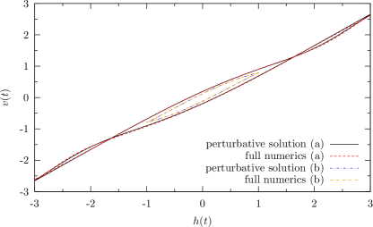
Figure 5: Comparison of the full numerical solution of equation (47) with the result obtained from the first non-vanishing perturbative order eq. (67) for (a) $h=3.0$, $c=3.0$, $\eta=1.5$ and (b) $h=1.0$, $c=1.0$, $\eta=0.6$. The units of $t$ and $z$ are chosen such that $\omega=\ell=1$.

The diagrammatic prescription yields up to terms of order ${\cal O}(\eta^{2})$

$$v(t)=h\cos\omega t+\eta^{2}\int\limits_{0}^{t}\text{d}t^{\prime}\>\text{e}^{-c(t-t^{\prime})}\Delta^{\prime}[Z(t)-Z(t^{\prime})].$$ (67)

A direct comparison of the numerical solution of (67) and the full equation of motion (47), shown in fig. 5, confirms an excellent agreement.

III.4 Perturbative harmonic expansion

For an ac driving force, even the lowest perturbative order for the velocity, equation (67) is a very complicated expression. We know from the numerics that, in the stationary state, the velocity is given by a periodic function with periodicity $\omega^{-1}$. This recommends to aim a harmonic expansion of the mean velocity $v$, i.e. to ask for the Fourier coefficients $a_{N}$ and $b_{N}$ in the ansatz

$$v(t)=\sum\limits_{N=1}^{\infty}\big{[}a_{N}\cos N\omega t+b_{N}\sin N\omega t\big{]},$$ (68)

It is now an important question, whether the first-order perturbative correction can further be simplified to get an analytic description of interesting features of the trajectory. One idea could be, to take only the lowest Fourier modes. In this section, we want to investigate, under which circumstances this could be possible.

Starting from the first order result for $v$, given by eq. (67), we express the disorder correlator by its Fourier transform

$$\Delta^{\prime}[Z(t)-Z(t^{\prime})]=\int\limits{\text{d}q\over 2\pi}(\text{i}q)\Delta(q)\text{e}^{\text{i}q{h\over\omega}[\sin\omega t-\sin\omega t^{\prime}]}$$ (69)

and expand the exponential term in a double Fourier series in $t$ and $t^{\prime}$, respectively:

$$\text{e}^{\text{i}a\sin\omega t} = \sum\limits_{n=-\infty}^{\infty}J_{n}(a)\text{e}^{\text{i}n\omega t}$$

$$\int\limits_{0}^{t}\text{d}t^{\prime}\>\text{e}^{-c(t-t^{\prime})-\text{i}a\sin\omega t^{\prime}} = \sum\limits_{n=-\infty}^{\infty}J_{n}(-a){\text{e}^{\text{i}n\omega t}-\text{e}^{-ct}\over c+\text{i}n\omega}.$$

Here, $J_{n}(a)$ are the Bessel functions of the first kind. As we are interested only in the behaviour for large enough times (the steady state solution), we remove all terms that are damped out exponentially for $t\gg c^{-1}$ from the very beginning. Note, that $c^{-1}$ is indeed the time scale for the transience, as has been claimed before.

For the mean velocity, we obtain

$$v(t)=h\cos\omega t+\eta^{2}\sum\limits_{m,n=-\infty}^{\infty}\int{\text{d}q\over 2\pi}(\text{i}q)\Delta(q)J_{m}\left(q{h\over\omega}\right)J_{n}\left(-q{h\over\omega}\right){\text{e}^{\text{i}(m+n)\omega t}(c-\text{i}n\omega)\over c^{2}+n^{2}\omega^{2}}.$$ (70)

In principle, this is already a Fourier series representation, not very elegant, though. The argument $(m+n)\omega t$ of the expansion basis exponentials promises a rather complicated structure for the coefficients. A first observation, however, can already be made: Under the $q$ integral we find an odd function $(\text{i}q)\Delta(q)$ and a product of two Bessel functions of order $m$ and $n$, respectively. For the $q$-integral to result in a finite value, a function is required that is not odd in $q$. This necessitates the product of the two Bessel functions to be odd, or, equivalently, $m+n$ to be an odd number. Whence, we conclude, that to first perturbative order, our symmetry argument (Fourier coefficients for even $N$ must vanish) is fulfilled exactly.

It requires some tedious algebra to collect all contributions belonging to a certain harmonic order from the double series. Eventually, we obtain a series expansion

$${{v}(t)\over h}=\cos\omega t+\sum\limits_{N=1}^{\infty}\bigg{[} A_{N}\left({\eta\over h},{\omega\over c},{h\over\omega\ell}\right)\cos N\omega t+$$

$$B_{N}\left({\eta\over h},{\omega\over c},{h\over\omega\ell}\right)\sin N\omega t\bigg{]}.$$ (71)

Note, that taking $\omega\to 0$ is forbidden here, as we used $\omega\neq 0$ while deriving the coefficients and moreover perturbation theory breaks down (recall that $h/\eta\gg c/\omega$). The same holds for $\ell\to 0$. The remaining extreme limits $\omega\to\infty$ and $\ell\to\infty$ are not interesting, since in these limits the disorder is rendered unimportant. Therefore, in the following, we assume finite (positive) values for $\ell$ and $\omega$ and moreover set them equal to one $\omega=\ell=1$, by appropriately choosing the units for $z$ and $t$.

Now, we are left with three dimensionless parameters: $h$, $c$ and $\eta$. The dependence of the first order perturbative Fourier coefficients on $\eta$ is trivial. The dependence on $c$ is also evident, as can be read off from (70). For larger $c$, the system is more tightly bound to the non-disordered solution, supressing perturbative corrections.

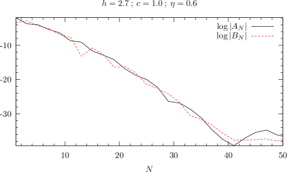
Figure 6: Plotting the logarithms of $|A_{N}|$ and $|B_{N}|$ reveals the exponential decay with $N$. In the regime where numerical errors do not dominate the result, a linear regression seems appropriate.

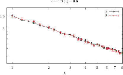
Figure 7: Performing the linear regression for many $h$ yields slopes $\alpha$ and $\beta$ appearing to depend on $h$ in a power-law fashion.

The most interesting but also the most difficult is the dependence of the Fourier coefficients on $h$. Actually, there are two competing effects. On the one hand, large driving strengths render the disorder unimportant in all cases accessible through perturbative methods. On the other hand, if one thinks of $g(Z(t))$ as a function of time, the more rapid $Z(t)$ changes the more $g$ fluctuates on short time scales and thus brings higher frequency contributions to $v(t)$. The first remark is reflected in the overall weight of the Fourier coefficients as corrections to the non-disordered case, decreasing with $h$. The second idea is expected to express itself in the decay of the Fourier coefficients with $N$. The larger $h$, the weaker we expect this decay to be.

The dependence of the higher harmonics on $h$ is hidden in the Bessel functions in (70). The first extremum of the Bessel functions shifts to larger values as $m$ and $n$ increase, respectively. However, the complicated way in which these Bessel functions enter $A_{N}$ and $B_{N}$ hinders an analytic access to the decay law. A numerical determination of the Fourier coefficients for the perturbative result reveals an exponential decay, as shown in fig. 6. The noisy behaviour for $N\geq 40$ is due to numerical fluctuations. Note, that these fluctuations are of the order $10^{-14}$, which is quite reasonable. The plot in fig. 6 is mere illustration of a more general phenomenon. This exponential decay has been found for many sets of parameters, thus one is led to the ansatz

$$|A_{N}|\sim{\eta^{2}\over h^{2}}\text{e}^{-\alpha N}\quad;\quad|B_{N}|\sim{\eta^{2}\over h^{2}}\text{e}^{-\beta N},$$ (72)

where $\alpha$ and $\beta$ can be estimated through a linear regression up to a suitable $N_{\text{max}}$. Of course, it is not expected, that $\alpha$ and $\beta$ are distinct, nor that they depend on the parameters in different ways. Determining both just doubles the amount of available data.

As our results are first-order perturbative, $\alpha$ and $\beta$ must not depend on $\eta$. The main interest now focusses on the dependence of the decay constants on $h$. The results from a linear regression for a series of $h$-values, $c$ and $\eta$ kept fixed, suggest a power-law dependence

$$\alpha(h,c)=C_{\alpha}(c)\cdot h^{-\xi_{\alpha}},\quad\beta(h,c)=C_{\beta}(c)\cdot h^{-\xi_{\beta}}.$$ (73)

Fig. 7 displays this relation for a particular example. Repeating this data collection and subsequent regression for different values for $c$ and $\eta$ yields the results summarised in table 1.

Table 1: Results for the regression (73).

$c$	$\eta$	$C_{\alpha}$	$C_{\beta}$	$\xi_{\alpha}$	$\xi_{\beta}$
1.0	0.6	1.52	1.52	0.61	0.61
1.5	0.6	1.56	1.56	0.58	0.59
2.0	0.6	1.56	1.59	0.58	0.60
2.5	0.6	1.63	1.62	0.61	0.61
3.0	1.0	1.66	1.66	0.63	0.63
3.5	1.0	1.71	1.68	0.62	0.62
4.0	1.0	1.69	1.65	0.61	0.60
4.5	1.0	1.72	1.68	0.62	0.62
5.0	2.0	1.71	1.67	0.61	0.60
5.5	2.0	1.73	1.73	0.61	0.62
6.0	2.0	1.77	1.72	0.62	0.62
6.5	3.0	1.76	1.77	0.62	0.62

While the exponent $\xi$ appears constant $\xi\approx 0.6$, the prefactor seems to depend on $c$.

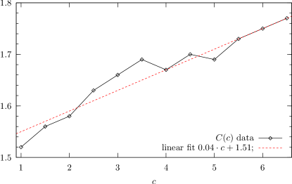
Figure 8: Plot of the change of the prefactor $C(c)=(C_{\alpha}+C_{\beta})/2$ in (73) on $c$. The linear fit yields a fairly tiny slope.

An attempt to redo the same procedure, done for $h$, with the parameter $c$ to gain information about the functional dependence of $\alpha$ and $\beta$ on $c$ yields a complicated but rather weak dependence, which gives no further insight. The linear fit in fig. 8 gives a fairly tiny slope, so the dependence of the decay constants on $c$ may be assumed to be weak.

Certainly, it is desirable to ascertain the validity of this decay law beyond perturbation theory. In a few words, it ought to be explained, why we have not been able to do it. First of all, the logarithmic plots of the Fourier coefficients in fig. 6 exhibit fluctuations around the linear decrease. This “noise” is authentic and not attributed to numerical inaccuracies. The exponential decay of the Fourier coefficients is superimposed on a true, complicated dependence. Hence, it requires a lot of data points to obtain reasonable data. Since the Fourier coefficients for even $N$ vanish, in the example of fig. 6 the regression can be carried out over around 15-20 data points. This is a fair number. The quality relies heavily on the accuracy of the numerical determination of the Fourier coefficients. In Fourier analyses of the numerics for the full equation of motion (47), we did not manage to get a precision better than of the order of $10^{-3}$. This means, the regression has to be stopped at $N_{\text{max}}$, where $\log A_{N_{\text{max}}}\approx-7$. In the example of fig. 6, this leaves us with less than 5 data points. In view of the natural fluctuations, a linear regression is not sensible any more.

In summary, we have numerically established the dependence of the decay constans for the Fourier coefficients on $h$: $\alpha,\beta(h)=C(c)\cdot h^{-\xi}$ with $\xi\simeq 0.6$.

IV Conclusions

We have seen that the perturbation expansion for ac-driven elastic interfaces in random media fails for interface dimensions $D\leq 4$. We have resolved this puzzle, and the reason for the strange behaviour of perturbation theory has been found to be connected with the disorder-dependent time scale $\tau$ (cf. (29)) which measures the time for the initial roughening of interfaces in random environments. Due to its appearence within the disorder averaged velocity $v$ as a transience relaxation time, attemps to determine $v$ via a perturbation expansion in the strength of the disorder entail terms of unbounded growth in time. Although, most probably, the expansion yields the true solution if it could be summed up, it is useless, because the finite perturbative orders grow in powers of time. They offer a good approximation to the full solution only on time scales small compared to the transience relaxation time and fail to describe correctly the behaviour on large time scales. On the other hand, as we have signified, the perturbation expansion for $D>4$ is regular.

Therefore, theoretical work towards an understanding of the important problem of ac-driven interfaces exposed to disorder has to take the route via the related mean-field problem. The mean-field equation of motion formally corresponds to $D=\infty$ and admits a regular perturbative treatment that, where applicable, agrees very well with the numerics for the full equation of motion. It has been shown, that non-regular diagrammatic contributions cancel among each other, leaving a well-behaved perturbative expansion.

Further, the solutions to the mean-field equation of motion have many features in common with the problem in finite dimension. Therefore, they can be useful to study some properties of the original problem, like the velocity-hysteretis.

The mean-field perturbation expansion helped to improve numerical results, which allowed us to establish the dependence of the decay constants of the Fourier modes on $h$ as a power law.

Appendix A The functional integral approach

Apart from a perturbative expansion of the equation of motion (2), it is also possible to compute the disorder averaged correlation functions via a functional integral approach Martin et al. (1973); De Dominicis (1978). Starting from (2)

$$\partial_{t}z_{x,t}=\Gamma\nabla_{x}^{2}z_{x,t}+h(t)+u\cdot g(x,z_{x,t})\equiv F[z_{x,t}]$$ (74)

(with $z_{x,t}$ being a short-hand notation for $z(x,t)$), we note that

$$\left\langle A[z_{x,t}]\right\rangle =\left\langle\int\mathcal{D}z_{x,t}\>A[z_{x,t}]\,\delta\Big{(}\partial_{t}z_{x,t}-F[z_{x,t}]\Big{)}\right\rangle$$ (75)

for any functional $A[z_{x,t}]$. Writing

$$\delta\Big{(}\partial_{t} z_{x,t}-F[z_{x,t}]\Big{)}$$

$$=\int\mathcal{D}\hat{z}_{x,t}\>\exp\left[\text{i}\int_{x,t}\hat{z}_{x,t}(\partial_{t}z_{x,t}-F[z_{x,t}])\right]$$ (76)

and using the usual cumulant expansion for Gaußian disorder, we find

$$\left\langle A[z_{x,t}]\right\rangle ={1\over\mathcal{Z}}\int\mathcal{D}\hat{z}_{x,t}\mathcal{D}z_{x,t}\>A[z_{x,t}]\,\text{e}^{\mathcal{S}[\hat{z},z]}$$ (77)

$$\mathcal{Z} =\int\mathcal{D}\hat{z}_{x,t}\mathcal{D}z_{x,t}\>\text{e}^{\mathcal{S}[\hat{z},z]}$$ (78)

$$\mathcal{S}[\hat{z},z] =\mathcal{S}_{0}[\hat{z},z]+\mathcal{S}_{h}[\hat{z},z]+\mathcal{S}_{\text{dis}}[\hat{z},z].$$ (79)

The three contributions to the action for this functional integral formula read

$$\mathcal{S}_{0}[\hat{z},z] =\text{i}\int_{x,t}\hat{z}_{x,t}\big{[}\partial_{t}-\Gamma\nabla_{x}^{2}\big{]}z_{x,t}$$ (80)

$$\mathcal{S}_{h}[\hat{z},z] =\text{i}\int_{x,t}\hat{z}_{x,t}h(t)$$ (81)

$$\mathcal{S}_{\text{dis}}[\hat{z},z] =-{u^{2}\over 2}\int_{x,t,t^{\prime}}\hat{z}_{x,t}\hat{z}_{x,t^{\prime}}\Delta[z_{x,t}-z_{x,t^{\prime}}].$$ (82)

Certainly, we can also compute correlation functions $A[z_{x,t},\hat{z}_{x^{\prime},t^{\prime}}]$. For example, we re-obtain the propagator (II.2) by calculating the response function

$$\text{i}\left\langle z_{x,t}\hat{z}_{x^{\prime},t^{\prime}}\right\rangle_{\mathcal{S}_{0}}=G(x-x^{\prime},t-t^{\prime}).$$ (83)

To set up a perturbative expansion in $u$, we decompose in the same way as in section II.2 $z_{x,t}=Z_{t}+\zeta_{x,t}$ with $Z_{t}=(h/\omega)\sin\omega t$. Instead of $z_{x,t}$ we now have to consider the functional integral over $\zeta_{x,t}$. Now

$$\mathcal{S}[\hat{z},\zeta] =\mathcal{S}_{0}[\hat{z},\zeta]+\mathcal{S}_{\text{dis}}[\hat{z},\zeta]$$ (84)

$$\mathcal{S}_{\text{dis}}[\hat{z},\zeta] =-{u^{2}\over 2}\int_{x,t,t^{\prime}}\hat{z}_{x,t}\hat{z}_{x,t^{\prime}}\Delta[Z_{t}+\zeta_{x,t}-Z_{t^{\prime}}-\zeta_{x,t^{\prime}}].$$ (85)

To compute correlation functions perturbatively in powers of $u$ requires to expand the normalisation $\mathcal{Z}$ as well. A small reflection shows that the lowest order contribution coming from $\mathcal{Z}$ is of order ${\cal O}(u^{4})$. Thus, if we want to calculate the velocity to order ${\cal O}(u^{2})$ we can ignore the $u$-dependence of $\mathcal{Z}$ and write

$$v(t) =h(t)+\partial_{t}\left\langle\zeta_{x,t}\right\rangle$$

$$=h(t)+\partial_{t}\left\langle\zeta_{x,t}\mathcal{S}_{\text{dis}}[\hat{z},\zeta]\right\rangle_{\mathcal{S}_{0}}+{\cal O}(u^{4}).$$ (86)

Of course, we may only retain $\mathcal{S}_{\text{dis}}[\hat{z},\zeta]$ up to terms of order ${\cal O}(u^{2})$, i.e.

$$\mathcal{S}_{\text{dis}}[\hat{z},\zeta] =-{u^{2}\over 2}\int_{x,t,t^{\prime}}\hat{z}_{x,t}\hat{z}_{x,t^{\prime}}\big{[}\Delta[Z_{t}-Z_{t^{\prime}}]+\Delta^{\prime}[Z_{t}-Z_{t^{\prime}}](\zeta_{x,t}-\zeta_{x,t^{\prime}})\big{]}+{\cal O}(u^{4}).$$ (87)

Averages with respect to $\mathcal{S}_{0}$ are Gaußian, thus Wick’s theorem applies and with (83) we recover the result from equation (13)

$$v(t) =h(t)-{u^{2}\over 2}\partial_{t}\int_{x^{\prime},t_{1},t_{2}}\Delta^{\prime}[Z_{t_{1}}-Z_{t_{2}}]\left\{\left\langle\zeta_{x,t}\hat{z}_{x^{\prime},t_{1}}\right\rangle_{\mathcal{S}_{0}}\left\langle\zeta_{x,t_{1}}\hat{z}_{x^{\prime},t_{2}}\right\rangle_{\mathcal{S}_{0}}-\left\langle\zeta_{x,t}\hat{z}_{x^{\prime},t_{2}}\right\rangle_{\mathcal{S}_{0}}\left\langle\zeta_{x,t_{2}}\hat{z}_{x^{\prime},t_{1}}\right\rangle_{\mathcal{S}_{0}}\right\}+{\cal O}(u^{4})$$

$$=h(t)-u^{2}\partial_{t}\int_{x^{\prime},t_{1},t_{2}}\Delta^{\prime}[Z_{t_{1}}-Z_{t_{2}}]\{-\text{i}G(x-x^{\prime},t-t_{1})\}\{-\text{i}G(x-x^{\prime},t_{1}-t_{2})]\}+{\cal O}(u^{4})$$

$$=h(t)+u^{2}\int_{t^{\prime}}\Delta^{\prime}[Z_{t}-Z_{t^{\prime}}]G(0,t-t^{\prime})+{\cal O}(u^{4}).$$ (88)

It is clear, that we can continue equation (A) to higher orders in $u$ by taking into account higher orders in $u$ of $\exp(\mathcal{S}_{\text{dis}})$ as well as higher order corrections from $\mathcal{Z}$. This way, it is possible to rearrive at the graphical expansion presented in section II.3, albeit along a little more complicated route.

Appendix B The regularity of all perturbative orders in case $D>4$

Let us start with an example graph at which we demonstrate the steps, that are then generalised further down. We consider the following fourth order contribution to the correction of the disorder averaged velocity

$$\parbox{71.13188pt}{\includegraphics{exdiag1.eps}}= \int\limits_{0}^{t}\text{d}t_{1}\int\limits_{0}^{t_{1}}\text{d}t_{2}\int\limits_{0}^{t_{2}}\text{d}t_{3}\prod\limits_{i=1}^{3}\int\text{d}^{D}x_{i}$$

$$G(x-x_{1},t-t_{1})G(x_{1}-x_{2},t_{1}-t_{2})G(x_{2}-x_{3},t_{2}-t_{3})\times$$

$$\delta(x-x_{2})\delta(x_{1}-x_{3})(-\Delta^{\prime\prime}[Z-Z_{2}])\Delta^{\prime}[Z_{1}-Z_{3}]$$ (89)

$$= \int\limits_{0}^{t}\text{d}t_{1}\int\limits_{0}^{t_{1}}\text{d}t_{2}\int\limits_{0}^{t_{2}}\text{d}t_{3}\>(-\Delta^{\prime\prime}[Z-Z_{2}])\Delta^{\prime}[Z_{1}-Z_{3}]\times$$

$$\int\text{d}^{D}x^{\prime}\>G(x-x^{\prime},t-t_{1})G(x^{\prime}-x,t_{1}-t_{2})G(x-x^{\prime},t_{2}-t_{3})$$ (90)

$$\int\text{d}^{D}x^{\prime}G(x-x^{\prime},t-t_{1}) G(x^{\prime}-x,t_{1}-t_{2})G(x-x^{\prime},t_{2}-t_{3})=$$

$$\int{\text{d}^{D}k_{1}\text{d}^{D}k_{2}\over(2\pi)^{2D}}\text{e}^{-\Gamma\big{[}k_{1}^{2}(t-t_{1})+(k_{1}+k_{2})^{2}(t_{1}-t_{2})+k_{2}^{2}(t_{2}-t_{3})\big{]}}$$ (91)

We can now assign momenta to the branches of the tree

$$\parbox{71.13188pt}{\includegraphics{exdiag2.eps}},$$ (92)

and we can read off from (B), that

$$k_{\alpha}=k_{1}\,,\quad k_{\beta}=k_{1}+k_{2}\,,\quad k_{\gamma}=k_{2}.$$ (93)

Obviously, $k_{1}$ describes the momentum “flowing” from the root to vertex 2 and $k_{2}$ is the momentum “flow” from vertex 1 to vertex 3. Estimating the disorder correlator derivatives in equation (B) by constants (that we can drop since they do not influence the asymptotics $t\to\infty$), all that has to be done is the integration of the right-hand side of (B) over the 3 time variables $t_{1}$, $t_{2}$ and $t_{3}$. We start with the outermost leaf, $t_{3}$, and have

$$\int\limits_{0}^{t_{2}}\text{d}t_{3}\>\text{e}^{-\Gamma k_{2}^{2}(t_{2}-t_{3})}={1\over\Gamma k_{2}^{2}}\left[1-\text{e}^{-\Gamma k_{2}^{2}t_{2}}\right]\leq{1\over\Gamma k_{2}^{2}}.$$ (94)

Proceeding in the same manner for the remaining time variables, we finally find

$$\bigg{|}\>\parbox{71.13188pt}{\includegraphics{exdiag1.eps}}\bigg{|}\leq \int{\text{d}^{D}k_{1}\text{d}^{D}k_{2}\over(2\pi)^{2D}}{1\over\Gamma^{3}k_{1}^{2}(k_{1}+k_{2})^{2}k_{2}^{2}}.$$ (95)

This is certainly finite for $D>4$.

Now, we turn to the general argument for all trees of general (even) order $2q$. Let ${\cal T}_{q}$ denote the set of all rooted trees with $q$ vertices, and ${\cal P}(T)$ all possible unordered pairings of vertices of $T\in{\cal T}_{q}$. Let moreover $B_{T}$ be the set of all branches of the tree $T$. We want to agree that a branch $b=(b_{1},b_{2})$ has $b_{1}$ always closer to the root. Then, we have in general for every order

$$\left\langle v_{2q}\right\rangle=\sum\limits_{T\in{\cal T}_{2q}}\sum\limits_{P\in{\cal P}(T)}A_{T,P}.$$ (96)

Here, $A_{T,P}$ is a single diagram, namely a tree $T$ where all pairs $(p_{1},p_{2})\in P$ are connected by dashed lines for the Gaußian disorder average. The disorder correlators that enter $A_{T,P}$ can be estimated by constants $|\Delta^{(m)}[Z^{\prime}-Z^{\prime\prime}]|\leq c_{m}\ell^{-m}$, that we drop in the following. They are finite and do not influence the behaviour of $A_{T,P}$ as $t\to\infty$. Denoting the root vertex by $r$, we estimate

$$|A_{T,P}|\leq \bigg{(}\prod\limits_{b\in B_{T}}\int{\text{d}^{D}k_{b}\over(2\pi)^{D}}\int\limits_{0}^{t_{b_{1}}}\text{d}t_{b_{2}}\int\text{d}^{D}x_{b_{2}}\bigg{)}\bigg{(}\prod\limits_{b\in B_{T}}\text{e}^{-\Gamma k_{b}^{2}(t_{b_{1}}-t_{b_{2}})+\text{i}k_{b}(x_{b_{1}}-x_{b_{2}})}\bigg{)}\prod\limits_{p\in P}\delta(x_{p_{1}}-x_{p_{2}})$$ (97)

$$= \bigg{(}\prod\limits_{b\in B_{T}}\int{\text{d}^{D}k_{b}\over(2\pi)^{D}}\int\limits_{0}^{t_{b_{1}}}\text{d}t_{b_{2}}\bigg{)}\bigg{(}\prod\limits_{p\in P\atop r\notin p}\int\text{d}^{D}x_{p_{1}}\bigg{)}\exp\bigg{[}-\Gamma\sum\limits_{b\in B_{T}}k_{b}^{2}(t_{b_{1}}-t_{b_{2}})$$

$$+\text{i}\sum\limits_{p\in P}x_{p_{1}}\sum\limits_{b\in B_{T}}k_{b}\left(\delta_{b_{1},p_{1}}+\delta_{b_{1},p_{2}}-\delta_{b_{2},p_{1}}-\delta_{b_{2},p_{2}}\right)\bigg{]}$$ (98)

The integration over the remaining $x$-coordinates brings delta-functions for the momenta:

$$|A_{T,P}|\leq \bigg{(}\prod\limits_{b\in B_{T}}\int{\text{d}^{D}k_{b}\over(2\pi)^{D}}\int\limits_{0}^{t_{b_{1}}}\text{d}t_{b_{2}}\bigg{)}\exp\bigg{[}-\Gamma\sum\limits_{b\in B_{T}}k_{b}^{2}(t_{b_{1}}-t_{b_{2}})\bigg{]}$$

$$\prod\limits_{p\in P\atop r\notin p}(2\pi)^{D}\delta\bigg{(}\sum\limits_{b\in B_{T}}k_{b}\left(\delta_{b_{1},p_{1}}+\delta_{b_{1},p_{2}}-\delta_{b_{2},p_{1}}-\delta_{b_{2},p_{2}}\right)\bigg{)}$$ (99)

The $q-1$ delta-functions for the momenta mean, that the net out-flow (away from the root) of momentum from a vertex $p_{1}$ equals the net in-flow of momentum for the Gaußian partner vertex $p_{2}$ (i.e. $(p_{1},p_{2})\in P$). There is no delta-function ensuring this for the root and its partner vertex. However, this is not needed. The root itself has only out-flow of momentum and that has to be absorbed by its partner vertex to ensure the balance for all other pairs. This explains, why no exponential function involving $x$ appears any more in (B). As a result, we can assign a momentum $k_{p}$ to each pair $P\ni p=(p_{1},p_{2})$, describing the net momentum transfer from the vertex $p_{1}$ to $p_{2}$. This insight advises to choose the momentum associated to the $q$ Gaußian pairs as the $q$ integration variables $k_{p}$. The momentum assigned to a bond $k_{b}$ denotes the total flow of momentum through this bond, determined by the source or drain properties of the bond boundary vertices $b_{1}$ and $b_{2}$. The rest is now easy, if we follow the estimate for the time integrals from the equation (94) in the example before. We end up with

$$|A_{T,P}|\leq \bigg{(}\prod\limits_{p\in P}\int{\text{d}^{D}k_{p}\over(2\pi)^{D}}\bigg{)}\prod\limits_{b\in B_{T}}{1\over\Gamma k_{b}^{2}}.$$ (100)

One first puzzle related to (100) is obvious: there may be bonds, that carry momentum $k_{b}=0$. This exactly happens for lines that connect to a subtree which has only internal Gaußian pairings, i.e. the whole momentum flow remains inside the subtree. Such lines are problematic in all dimensions, even in the mean-field theory, where they correspond to the curly lines in the graphical expansion for the mean-field equation of motion (cf. section III.3). The resolution of this problem by cancellations among several such diagrams is technically a little easier for the mean-field case, where we performed it (cf. section III.3.2 and appendix E). The idea of the mean-field proof exactly applies here as well, just in mean-field we do not carry the load of momentum integrals. The adaption of the proof itself is straightforward.

Another problem in connection with (100) is the fact, that we have only $q$ momenta to integrate over but $2q-1$ bonds. So for every given order it happens for a couple of diagrams, that some momentum, $k_{p}$ say, appears to the power $k_{p}^{-2q}$ in (100). Thus, the integration over $k_{p}$ has infrared problems in $D\leq 2q$, but integration over the other momenta works in $D>2$. Actually, this problem can again be resolved by summing several such diagrams in multiple steps. After the first step, one obtains a result, that has $k_{p}$ divergent in $D\leq 2q-2$ but another momentum, $k_{p^{\prime}}$ say, divergent in $D\leq 4$ instead of $D\leq 2$. So, viewed as a function of $k_{p}$ the intermediate result is better behaved, but worse for $k_{p^{\prime}}$. Let us take a closer look at this. We start with a glimpse on this issue for the expansion of $\left\langle v_{6}\right\rangle$, where we have checked that everything remains bounded in $D>4$. The expansion of $\left\langle v_{6}\right\rangle$ contains, among others, the following diagrams

$$D_{1}^{6} =\parbox{71.13188pt}{\includegraphics{hodiag1.eps}}$$ (101)

$$D_{2}^{6} =\parbox{93.89409pt}{\includegraphics{hodiag2.eps}}$$ (102)

$$D_{3}^{6} =\parbox{93.89409pt}{\includegraphics{hodiag3.eps}}$$ (103)

$$D_{4}^{6} =\parbox{116.6563pt}{\includegraphics{hodiag4.eps}}.$$ (104)

With regard to their topological structure, these are the only diagrams that have problems in $D>4$, other such diagrams are constructed from them by a different choice of the root. Incidentally, $D_{2}^{6}$ and $D_{3}^{6}$ are topologically equivalent as well. We can easily see that in each diagram $D_{1}^{6},\ldots,D_{4}^{6}$, there are 3 bonds that carry the momentum $k_{1}$ belonging to the pair of the root and the outermost vertex. The momenta associated to the other two Gaußian pairs, $k_{2}$ and $k_{3}$, occur only within exactly one bond. Thus, according to equation (100) the integration over $k_{1}$ produces problems in $D\leq 6$, whereas integration over $k_{2}$ and $k_{3}$ is harmless in $D>2$. One can now check, that the sum $4D^{6}_{1}+2D^{6}_{2}$ as well as the sum of $2D^{6}_{3}+D^{6}_{4}$ is regular in $D>4$. The factors that I have put count the incidence of each diagram in the expansion.

The mechanism of combining diagrams to improve the properties with respect to integration over some $k_{i}$ and make it worse for some other $k_{j}$ can already be demonstrated at graphs of order $4$. If, from $D^{6}_{1}$ and $D^{6}_{2}$ the root and the upper vertex closest to the root are removed and the outermost leaf connected to the new root, we have the two diagrams of fourth order (cf. (23))

$$2D_{1}^{4} =2\cdot\>\parbox{48.36967pt}{\includegraphics{4odiag1.eps}}$$

$$=\int_{k_{1},k_{2}}\int\limits_{0}^{t}\text{d}t_{1}\>\text{e}^{-\Gamma k_{1}^{2}(t-t_{1})}\int\limits_{0}^{t_{1}}\text{d}t_{2}\>\text{e}^{-\Gamma k_{2}^{2}(t_{1}-t_{2})}\Delta^{\prime\prime}[Z_{1}-Z_{2}]\int\limits_{0}^{t_{1}}\text{d}t_{3}\>\text{e}^{-\Gamma k_{1}^{2}(t_{1}-t_{3})}\Delta^{\prime}[Z-Z_{3}]$$ (105)

$$D_{2}^{4} =\>\parbox{71.13188pt}{\includegraphics{4odiag2.eps}}$$

$$=-\int_{k_{1},k_{2}}\int\limits_{0}^{t}\text{d}t_{1}\>\text{e}^{-\Gamma k_{1}^{2}(t-t_{1})}\int\limits_{0}^{t_{1}}\text{d}t_{2}\>\text{e}^{-\Gamma k_{2}^{2}(t_{1}-t_{2})}\Delta^{\prime\prime}[Z_{1}-Z_{2}]\int\limits_{0}^{t_{2}}\text{d}t_{3}\>\text{e}^{-\Gamma k_{1}^{2}(t_{2}-t_{3})}\Delta^{\prime}[Z-Z_{3}]$$ (106)

$$=-2\cdot\>\parbox{48.36967pt}{\includegraphics{4odiag1.eps}}+S$$ (107)

$$S =\int_{k_{1},k_{2}}\int\limits_{0}^{t}\text{d}t_{1}\>\text{e}^{-\Gamma k_{1}^{2}(t-t_{1})}\int\limits_{0}^{t_{1}}\text{d}t_{2}\>\text{e}^{-\Gamma k_{2}^{2}(t_{1}-t_{2})}\Delta^{\prime}[Z-Z_{2}]\int\limits_{0}^{t_{2}}\text{d}\tau\>\text{e}^{-\Gamma k_{1}^{2}(t_{2}-\tau)}\Delta^{\prime\prime}[Z_{1}-Z(\tau)]$$

$$\phantom{=}-\int_{k_{1},k_{2}}\int\limits_{0}^{t}\text{d}t_{1}\>\text{e}^{-\Gamma k_{1}^{2}(t-t_{1})}\int\limits_{0}^{t_{1}}\text{d}t_{2}\>\text{e}^{-\Gamma k_{2}^{2}(t_{1}-t_{2})}\Gamma k_{1}^{2}\int\limits_{0}^{t_{2}}\text{d}t_{3}\text{e}^{-\Gamma k_{1}^{2}(t_{2}-t_{3})}\Delta^{\prime}[Z-Z_{3}]\times$$

$$\phantom{=}\int\limits_{0}^{t_{2}}\text{d}\tau\>\text{e}^{-\Gamma k_{1}^{2}(t_{2}-\tau)}\Delta^{\prime\prime}[Z_{1}-Z(\tau)]$$ (108)

The modification of $D_{2}^{4}$ relies on integration by parts for the integral over $t_{2}$. Upon inspection of the integrals, one sees, that the integral over $k_{1}$ in the diagrams $D_{1}^{4}$ and $D_{2}^{4}$ is well-behaved for $t\to\infty$ in $D>4$, while the integral over $k_{2}$ requires only $D>2$. The sum $S=2D_{1}^{4}+D_{2}^{4}$ on the other hand behaves vice versa. Of course, in expressions of order $4$ not much is gained with that, but in higher orders this procedure can be used to understand, why the sum of all diagrams of a certain order $2q$ involves $q-1$ integrals over momenta that are finite as $t\to\infty$ in $D>4$ and one that works in $D>2$. Note, that in equations (B-B) it is important to retain the disorder correlators, because cancellations have to be exact.

It is now easy to extend the calculations provided in (B-B) to see that $4D^{6}_{1}+2D^{6}_{2}$ (cf. equations (101) and (102)) is a regular expression in $D>4$. The sum $4D^{6}_{1}+2D^{6}_{2}$ has the critical dimension for $k_{1}$, the momentum associated to the Gaußian pair made of the root and the outermost leaf, reduced so that it is regular in $D>4$ at the price that now $k_{3}$ also needs $D>4$ instead of $D>2$. For reasons of space, as the explicit expressions for the diagrams are rather huge, we do not provide the full calculation here.

The more general idea about the cancellation among trees goes as follows. Because too many details have to be ascertained which tends to result in a huge load of technicalities, we will merely sketch the procedure by mentioning all intermediate steps without proving the implicit claims. First of all, we note, that any tree $T$ involves at least one distinguished momentum, we denote it by $k_{T}$, the integration over which is regular in $D>2$. In (B-B) we have seen that it is possible for any tree $T_{q}$ of any given order $q$, that is regular in $D>4$, to find partner trees $T_{q}^{1},\ldots,T_{q}^{m}$ of the same order, all regular in $D>4$, such that their sum is an expression in which the momentum associated to the root has the property of $k_{T}$. Thus, we will without loss of generality assume that for any tree that is regular in $D>4$, $k_{T}$ is the momentum flowing out of the root. All our arguments in the following will also hold for trees for which this is not the case, if we repeat it for all partner trees and take the sum.

Let, for some tree $T$ the integration over some momentum $k_{p}$ associated to a Gaußian pair $p$ be problematic in $D>2N_{0}+2$. This can happen if along the line from $p_{1}$ to $p_{2}$ there are $N_{0}$ vertices which form the root of independent subtrees $\{S_{i}\}$ or if the momentum flow along the route from $p_{1}$ to $p_{2}$ is interrupted by $N_{0}$ independent (w.r.t. the disorder average) inner subtrees $\{S_{i}\}$ and continues at the Gaußian partner of the root of those subtrees. The first case corresponds to the diagram $D_{1}^{6}$ given by (101) and the second scenario is exemplified by $D_{4}^{6}$ which is depicted in (104) (both for $N_{0}=2$). Of course, also a mixture of both events, $N_{0}$ in total, has the same effect, as is illustrated by $D_{2}^{6}$ and $D_{3}^{6}$. If, as a kind of induction hypothesis, we assume that all independent subtrees $S_{1},\ldots,S_{N_{0}}$ are regular in $D>4$, we can describe the scheme how to find all trees that have to be added to $T$ to yield an expression that is regular in $D>4$. Let us consider first $N_{0}=2$. Let $s_{1}$ be the root of $S_{1}$ and $s_{1}^{\prime}$ be its Gaußian partner vertex in $S_{1}$. As mentioned above, the integration over the momentum $k_{s}$, associated to $(s_{1},s_{1}^{\prime})$, is regular in $D>2$. Without loss of generality, we assume that in $T$, $s_{1}$ is a vertex on the non-interrupted path from $p_{1}$ to $p_{2}$. Then there is another tree $T^{\prime}$, for which the flow of $k_{p}$ along the connection between $p_{1}$ and $p_{2}$ is interrupted by the connection between $s_{1}$ and $s_{1}^{\prime}$. The sum of $T$ and $T^{\prime}$ is then regular in $D>4$. The integral over $k_{p}$ in the sum $T+T^{\prime}$ has decreased its critical dimension by 2 at the cost, that now the integration over $k_{s}$ needs $D>4$ to be bounded for large $t$.

So far, this is the idea, how the cancellation among trees works in $D>4$ to give a regular expression. For a thorough proof, we would have to give evidence for each single intermediate step. After all, the practical benefit of such a detailed proof is little and no further insight can be expected. Thus, although a rigorous proof has not been established, a consistent picture of the behaviour of the perturbation expansion has emerged. In $D>4$ all perturbative orders are regular, and in $D\leq 4$ our somewhat crude estimate of the disorder correlator derivatives by constants gives bad results.

Appendix C Analysis of the bush graphs

To analyse the term

$$T_{1} =\int\limits_{0}^{t}\text{d}t_{1}\text{d}t_{2}\>\Delta[Z_{1}-Z_{2}]\int{\text{d}^{D}k\over(2\pi)^{D}}\>\text{e}^{-\Gamma k^{2}(2t-t_{1}-t_{2})}$$ (109)

from equation (II.4), we start with the decomposition of the function $\Delta[Z(t_{1})-Z(t_{2})]$ in a double Fourier series in $t_{1}$ and $t_{2}$, respectively. Recall, that $Z(t)=(h/\omega)\sin\omega t$.

$$\Delta[Z(t_{1})-Z(t_{2})]=\int_{q}\hat{\Delta}(q)\sum\limits_{m,n} J_{m}(qh/\omega)J_{n}(-qh/\omega)\times$$

$$\text{e}^{\text{i}\omega(mt_{1}+nt_{2})}.$$ (110)

Here, $\hat{\Delta}$ is the Fourier transform of $\Delta$ and $J_{m}$ is the Bessel function of the first kind. For symmetry reasons, only terms with an even value of $m+n$ contribute. This gives

$$T_{1}=\int_{q}\hat{\Delta}(q)\bigg{[} L_{0,0}(q,t)+\sum\limits_{m\neq 0}L_{2m,0}(q,t)+$$

$$\sum\limits_{m,n\neq 0}L_{m,n}(q,t)\bigg{]},$$ (111)

where we have introduced

$$L_{m,n}(q,t)= J_{m}\left({qh\over\omega}\right)J_{n}\left(-{qh\over\omega}\right)\int\limits_{0}^{t}\text{d}t_{1}\text{d}t_{2}\>\text{e}^{\text{i}\omega(mt_{1}+nt_{2})}$$

$$\int{\text{d}^{D}k\over(2\pi)^{D}}\>\text{e}^{-\Gamma k^{2}(2t-t_{2}-t_{2})}$$

$$= J_{m}\left({qh\over\omega}\right)J_{n}\left(-{qh\over\omega}\right)\times$$

$$\int{\text{d}^{D}k\over(2\pi)^{D}}\>{\left[\text{e}^{\text{i}m\omega t}-\text{e}^{-\Gamma k^{2}t}\right]\over\Gamma k^{2}+\text{i}m\omega}{\left[\text{e}^{\text{i}n\omega t}-\text{e}^{-\Gamma k^{2}t}\right]\over\Gamma k^{2}+\text{i}n\omega}.$$ (112)

The behaviour for $t\to\infty$ is dominated by the leading term $L_{0,0}(q,t)$, which is given by

$$L_{0,0}(q,t) =J_{0}^{2}\left({qh\over\omega}\right){S_{D}\over\Gamma^{2}(2\pi)^{D}}\int\limits_{0}^{\Lambda}\text{d}k\>k^{D-5}\left[1-\text{e}^{-\Gamma k^{2}t}\right]^{2}$$

$$=J_{0}^{2}\left({qh\over\omega}\right)\>{t^{4-D\over 2}\over\Gamma^{D\over 2}}\>A_{D}(t/\vartheta).$$ (113)

The function $A_{D}(x)$ has already been introduced in equation (31). The sub-leading terms are given by

$$L_{2m,0}= J_{0}\left({qh\over\omega}\right)J_{2m}\left({qh\over\omega}\right)\times$$

$$\int{\text{d}^{D}k\over(2\pi)^{D}}\>{\left[1-\text{e}^{-\Gamma k^{2}t}\right]\over\Gamma k^{2}}{\left[\text{e}^{\text{i}2m\omega t}-\text{e}^{-\Gamma k^{2}t}\right]\over\Gamma k^{2}+\text{i}2m\omega}.$$ (114)

Thus,

$$\sum\limits_{m\neq 0} L_{2m,0}(q,t)=$$

$$\sum\limits_{m=1}^{\infty}J_{0}\left({qh\over\omega}\right)J_{2m}\left({qh\over\omega}\right){t^{2-D\over 2}\over\omega\Gamma^{D\over 2}}\alpha_{D}^{m}(t/\vartheta,\omega t).$$ (115)

Here, the function $\alpha_{D}^{m}(x,y)$ is given by

$$\alpha_{D}^{m}(x,y)= {2S_{D}\over(2\pi)^{D}}\int\limits_{0}^{\sqrt{x}}\text{d}p\>p^{D-3}\left[1-\text{e}^{-p^{2}}\right]\times$$

$${{p\over y}\cos 2my+2m\sin 2my-{p\over y}\text{e}^{-p}\over(p^{2}/y^{2})+4m^{2}},$$ (116)

which, for $x\to\infty$ behaves in the same way, as $a_{D}(x)$ (cf. (18)), independent of $m\neq 0$.

The last term in (C) does not require further consideration. For $m,n\neq 0$, the function $L_{m,n}$ remains finite as $t\to\infty$. There is no infrared problem with the $k$-integral in equation (C) any more. Recalling the two time scales $\tau$ and $\vartheta$, that we have encountered before (cf. (29) and (30)) we thus have

$${u^{2}\over\ell^{2}}T_{1}= \left({t\over\tau}\right)^{4-D\over 2}\kappa_{D}\left({t\over\vartheta}\right)+$$

$$\left({t\over\tau}\right)^{4-D\over 4}{u\Lambda^{D\over 2}\over\omega\ell}k_{D}\left({t\over\vartheta},\omega t\right)+$$

$${u^{2}\Lambda^{D}\over\omega^{2}\ell^{2}}P_{D}\left({t\over\vartheta},\omega t\right).$$ (117)

Hereby, we have introduced

$$\kappa_{D}\left({t\over\vartheta}\right)= A_{D}(t/\vartheta)\int_{q}\hat{\Delta}(q)J_{0}^{2}\left({qh\over\omega}\right)$$ (118)

$$k_{D}\left({t\over\vartheta},\omega t\right)= \left({\vartheta\over t}\right)^{D\over 4}\sum\limits_{m=1}^{\infty}\alpha_{D}^{m}\left({t\over\vartheta},\omega t\right)\times$$

$$\int_{q}\hat{\Delta}(q)J_{0}\left({qh\over\omega}\right)J_{2m}\left({qh\over\omega}\right)$$ (119)

$$P_{D}\left({t\over\vartheta},\omega t\right)= {\omega^{2}\over\Lambda^{D}}\sum\limits_{m,n\neq 0}\int_{q}\hat{\Delta}(q)L_{m,n}(q,t).$$ (120)

The second factor in (II.4)

$$T_{2}=\int\limits_{0}^{t}\text{d}t^{\prime}\>\Delta^{(2p-1)}[Z-Z^{\prime}]\int{\text{d}^{D}k\over(2\pi)^{D}}\>\text{e}^{-\Gamma k^{2}(t-t^{\prime})}$$ (121)

can be treated in the same way, like the second order graph in section II.2, by splitting off the Fourier-0-mode

$$\Delta^{(2p-1)}[Z(t)-Z(t^{\prime})] ={F_{0}^{[2p-1]}(\omega t)+p(t,t^{\prime})\over\ell^{2p-1}}.$$ (122)

Following the calculations in section II.2, with $F_{0}(\omega t)$ replaced by $F_{0}^{[2p-1]}(\omega t)$, we arrive at

$${u^{2}\ell^{2(p-1)}\over\omega\ell}T_{2}= {u\Lambda^{D\over 2}\over\omega\ell}\left({t\over\tau}\right)^{4-D\over 4}f_{D}\left({t\over\vartheta},\omega t\right)+$$

$${u^{2}\Lambda^{D}\over\omega^{2}\ell^{2}}p_{D}\left({t\over\vartheta},\omega t\right),$$ (123)

where

$$f_{D}\left({t\over\vartheta},\omega t\right)= \left({\vartheta\over t}\right)^{D\over 4}a_{D}(t/\vartheta)F_{0}^{[2p-1]}(\omega t)$$ (124)

$$p_{D}\left({t\over\vartheta},\omega t\right)= {S_{D}\over(2\pi)^{D}}\int\limits_{0}^{\sqrt{t/\vartheta}}\text{d}p\>p^{D-1}\text{e}^{-p^{2}}\int\limits_{0}^{t}\text{d}t^{\prime}\>{p(t,t-t^{\prime})\over[\Gamma t^{\prime}]^{D}}.$$ (125)

The integral over $p$ in $p_{D}$ is certainly convergent for any $D$ in the limit $t\to\infty$, and the integral over $t^{\prime}$ converges for any $D>0$, since $p(t,t-t^{\prime})$ is a bounded oscillation around zero (without zero Fourier mode) in $t^{\prime}$.

Appendix D The width of ac-driven interfaces

Apart from the velocity of the mean position of an interface in a random potential, there is another interesting quantity that deserves investigation: the mean square deviation of a given realisation from the mean. More precisely, we refer to the quantity

$$w=\left\langle(\left\langle z\right\rangle-z)^{2}\right\rangle.$$ (126)

In the first order of the perturbation expansion, $w$ reads

$$w=\left\langle(\left\langle Z+u\zeta_{1}\right\rangle-Z-u\zeta_{1})^{2}\right\rangle=u^{2}\left\langle\zeta_{1}^{2}\right\rangle+{\cal O}(u^{4}).$$ (127)

In the case of infinitely extended interfaces, this quantity measures thus the typical width of the interface.

So, for infinitely extended domain walls, the typical width to first order in perturbation theory is given by (cf. (11))

$$\left\langle\zeta_{1}^{2}\right\rangle(x,t)=\int\limits_{0}^{t}\text{d}t_{1}\text{d}t_{2}\> \Delta[Z(t_{1})-Z(t_{2})]\times$$

$$\int{\text{d}^{D}k\over(2\pi)^{D}}\>\text{e}^{-\Gamma k^{2}(2t-t_{1}-t_{2})}.$$ (128)

Comparing this to $T_{1}$, given by equation (27), we find $\left\langle\zeta_{1}^{2}\right\rangle=T_{1}$. Using equation (II.4), we thus have for the asymptotics $t\to\infty$

$$u^{2}\left\langle\zeta_{1}^{2}\right\rangle\sim\ell^{2}\left[{t\over\tau}\right]^{4-D\over 2}A_{D}(t/\vartheta)$$ (129)

The function $A_{D}$, given by (31), remains bounded for $D<4$ and grows logarithmically in its argument in case $D=4$. Thus, the growth of the perturbative estimate of $w$ in time is given by the prefactor $t^{4-D\over 2}$ and $\log t$ for $D<4$ and $D=4$, respectively.

So, in contrast to the first order perturbative result for the interface’s velocity, which remains finite as $t\to\infty$ for $D>2$, the width of the interface indicates the correct critical dimension $D=4$ already to first order.

Appendix E Regularity of the mean-field perturbation expansion

In section III.3.2 we have analysed, how the unbounded contributions, contained in the two diagrams that involve a curly line, mutually cancel in the second non-vanishing perturbative order. In this appendix, we are going to explain how this cancellation process generalises to all orders in perturbation theory. As before, for simplicity, we work with the diagrams for the disorder-averaged velocity, that arise by just removing the curly lines from the root of the diagrams for $\left\langle\zeta\right\rangle$ (cf. equation (III.3.1)). In a velocity diagram contributing to the $n$-th order (recall, that only for even $n$ the corrections are non-zero), any curly line connects two trees of order $p$ and $q$ (both even) with the restriction $p+q=n$. Both trees appear in the expansion of lower orders, namely $p$ and $q$, respectively. In the following, we sketch an inductive proof for the claim that the unbounded terms originating from trees with curly internal lines cancel among each other.

Let us assume, that for order $n$ we have achieved to ensure regularity. For every unbounded tree $T$, there is thus a set $T^{1},\ldots,T^{a}$ of, let us call them cancelling trees, such that $T+T^{1}+\ldots+T^{a}$ is a regular, bounded expression in time. As a starting point for the induction, take $n=4$, where the validity of the claim has been verified in section III.3.2. It is now the task to validate the regularity for order $n+2$. First of all, we consider the process of attaching the root of a regular tree $S$ (with no internal curly line) of order $s$ by a curly line to a vertex $v$ of another regular tree $R$ of order $r=n+2-s$ to obtain a new irregular tree $A$ of order $n+2$. The vertex $v$ must be connected to another vertex $w\in R$ by a dashed line, to carry out the Gaußian disorder average. Without loss of generality, we assume that $v$ is connected to $w$ by a path that first makes a step towards the root. The rules for the diagrammatic expansion ensure, that there is a maximal regular subtree $T\subset R$, which contains $v$ and $w$.

Using partial integration, it is possible to move the vertex to which $S$ is connected (via the curly line) to a neighbouring vertex in $T$. Thus, it is possible to move the connection vertex along the unique way (in $T$) from $v$ to $w$. We are going to show, that once $w$ is reached, we have obtained the cancelling tree which is unique. Diagrammatcially, the process of moving the connection vertex from $v$ to $w$ reads:

$$= \>\>\parbox{59.75078pt}{\includegraphics{cdiag2.eps}}+D$$ (130)

Here, the blank circle represents $S$, the lightgrey circle stands for the subtree $R_{1}$ of $R$, to which $v$ connects and the darkgrey shaded circle denotes trees which run out of $v$ (summarised in the following as $R_{2}$). Certainly, in general there may be dashed lines between the dark- and the lightgrey circle, which we have omitted as they are not relevant for the forthcoming discussion. The dotted line just serves as a joker - it is not important to specify how many lines go out of $v$. The last term $D$ collects the left-over terms from the partial integration. Note, that, if it takes several steps to go from $v$ to $w$, the intermediate expressions (in the partial integration) are not in accordance with our diagrammatic rules, because the order of derivative of the disorder correlators does not appear correctly (it remains the same but the graph has changed). Keeping this small peculiarity in mind, it is nevertheless instructive to think in diagrammatic terms.

To illustrate the procedure, we take a look at the first step:

$$\parbox{59.75078pt}{\includegraphics{cdiag1.eps}}= R_{1}(t)\int\limits_{0}^{T_{1}}\text{d}t_{1}\>\text{e}^{-c(T_{1}-t_{1})}(-1)^{\nu}\Delta^{(\mu+\nu)}[Z(\tau)-Z(t_{1})]R_{2}(t_{1})\int\limits_{0}^{t_{1}}\text{d}t_{2}S(t_{2})$$ (131)

$$= R_{1}(t)\int\limits_{0}^{T_{1}}\text{d}t_{2}S(t_{2})\int\limits_{0}^{T_{1}}\text{d}t_{1}\text{e}^{-c(T_{1}-t_{1})}(-1)^{\nu}\Delta^{(\mu+\nu)}[Z(\tau)-Z(t_{1})]R_{2}(t_{1})$$

$$-R_{1}(t)\int\limits_{0}^{T_{1}}\text{d}t_{1}\>\text{e}^{-c(T_{1}-t_{1})}S(t_{1})\int\limits_{0}^{t_{1}}\text{d}t_{2}\>\text{e}^{-c(t_{1}-t_{2})}(-1)^{\nu}\Delta^{(\mu+\nu)}[Z(\tau)-Z(t_{2})]R_{2}(t_{2})$$ (132)

The order of the derivative (i.e. the number of outgoing lines) of $w$ and $v$ are denoted by $\mu$ and $\nu$, respectively. The time, at which the whole diagram is to be evaluated, is $t$, the time corresponding to the vertex to which $v$ is connected is given by $T_{1}$, $t_{1}$ is thus the time associated to $v$ and so on. The time of $w$ is $\tau$. Thus, we see, that if $w$ is not the vertex to which $v$ is directly connected (then $T_{1}\neq\tau$ in general), the first expression after partial integration cannot be a valid diagram: $v$ has lost one order of derivative ($\nu-1$ lines go out instead of $\nu$), but the derivative of the correlator $\Delta$ has not changed. A valid diagram however reappears, when the connection of $S$ has reached $w$. Then, $v$ has lost an outgoing line, but $w$ received one more and we indeed have achieved a cancelling tree: the factor $(-1)^{\nu}$ remains, the true diagram, however, has $(-1)^{\nu-1}$. The signs are different, thus the two trees cancel. The left-over term from the partial integration is again regular. This can be seen because all time integrals carry an exponential damping term. It is clear, that this is generally true for every partial integration step.

To go one step further, we assume now $S$ to be irregular. Essentially, the same procedure works, but there are more cancelling trees: one has take all cancelling trees $\{S^{i}\}$ for $S$ into account (which exist by induction hypothesis), thus $S$ is replaced by $\sum S^{i}$ and thence the left-over terms are again regular.

A possible irregularity of $R$ can be accounted for in the same way. It is, however, important to explain why this is possible, i.e. what are $v$ and $w$ in the cancelling trees for $R$. In the case of irregular $S$ the problem was easy, since all trees have a unique root. As we have seen already, the procedure of creating cancelling trees does not change the structure of regular subtrees. Thence, all cancelling trees for $R$ contain $T$. This makes clear, which $v$ and $w$ have to be chosen in the cancelling trees: they are well-defined in $T$ and $T$ is a well-defined subtree of the cancelling trees. Thus, repeating the whole procedure described above for all cancelling trees of $R$ yields the complete set of cancelling trees for $A$ in the most general setting.

Appendix F List of recurrent symbols

Symbol	Quantity	Reference
$z(x,t)$	interface profile	Sec.II.1
$D$	internal interface dimension	Sec.II.1
$h$	amplitude of the driving force	Eq.(1) and Eq.(2)
$\omega$	frequency of the ac-driving force	Eq.(1)
$\Gamma$	elastic stiffness of the interface	Eq.(2)
$c$	elasticity constant (mean-field)	Sec.III.1 and Eq.(47)
$\ell$	disorder correlation length	Sec.II.1 and Eq.(5)
$u$	disorder strength	Eq.(2)
$\eta$	disorder strength (mean-field)	Sec.III.1 and Eq.(2)
$\Delta$	disorder correlator	Sec.II.1 and Eq.(5) and Sec.III.1
$g$	disorder configuration	Eq.(2) and Eq.(47)
$L_{\text{p}}$	Larkin length	Eq.(6)
$Z(t)$	solution in absence of disorder	Sec.II.2 and Sec.III.3
$\zeta$	disorder correction to the solution	Sec.II.2 and Sec.III.3
$G$	propagator	Eq.(II.2) and Eq.(57)
$\Lambda$	inverse smallest length scale (UV-cutoff)	Sec.II.2
$\tau$	roughening time	Sec.II.4 and Eq.(29)
$\vartheta$	additional transience time scale	Sec.II.4 and Eq.(30)

References

- Kardar (1998) M. Kardar, Phys. Rep. 301, 85 (1998).
- Fisher (1998) D. S. Fisher, Phys. Rep. 301, 113 (1998).
- Brazovskii and Nattermann (2004) S. Brazovskii and T. Nattermann, Adv. Phys. 53, 177 (2004).
- Chauve et al. (2000) P. Chauve, T. Giamarchi, and P. Le Doussal, Phys. Rev. B 62, 6241 (2000).
- Kleemann et al. (2007) W. Kleemann et al., Phys. Rev. Lett. 99, 097203 (2007), and references therein.
- Kleemann (2007) W. Kleemann, Annu. Rev. Mater. Res. 37, 415 (2007).
- Jeżewski et al. (2008) W. Jeżewski, W. Kuczyński, and J. Hoffmann, Phys. Rev. B 77, 094101 (2008).
- Lyuksyutov et al. (1999) I. F. Lyuksyutov, T. Nattermann, and V. Pokrovsky, Phys. Rev. B 59, 4260 (1999).
- Nattermann et al. (2001) T. Nattermann, V. Pokrovsky, and V. M. Vinokur, Phys. Rev. Lett. 87, 197005 (2001).
- Fedorenko et al. (2004) A. A. Fedorenko, V. Mueller, and S. Stepanow, Phys. Rev. B 70, 224104 (2004).
- Glatz et al. (2003) A. Glatz, T. Nattermann, and V. Pokrovsky, Phys. Rev. Lett. 90, 047201 (2003).
- Glatz (2004) A. Glatz, Ph.D. thesis, Universität zu Köln (2004).
- Petracic et al. (2004) O. Petracic, A. Glatz, and W. Kleemann, Phys. Rev. B 70, 214432 (2004).
- Bender and Orszag (1978) C. M. Bender and S. A. Orszag, Advanced mathematical methods for scientists and engineers (McGraw-Hill, New York, 1978).
- Imry and Ma (1975) Y. Imry and S. K. Ma, Phys. Rev. Lett. 35, 1399 (1975).
- Imbrie (1984) J. Z. Imbrie, Phys. Rev. Lett. 53, 1747 (1984).
- Imbrie (1985) J. Z. Imbrie, Comm. Math. Phys. 98, 145 (1985).
- Fisher (1986) D. S. Fisher, Phys. Rev. Lett. 56, 1964 (1986).
- Villain (1988) J. Villain, J. Phys. A 21, L1099 (1988).
- Larkin (1970) A. I. Larkin, Sov. Phys. JETP 31, 784 (1970).
- Villain and Séméria (1983) J. Villain and B. Séméria, J. Physique Lett. 44, 889 (1983).
- Engel (1985) A. Engel, J. Physique Lett. 46, 409 (1985).
- Nattermann et al. (1992) T. Nattermann, S. Stepanow, L. H. Tang, and H. Leschhorn, J. Phys. II France 2, 1483 (1992).
- Narayan and Fisher (1992) O. Narayan and D. S. Fisher, Phys. Rev. B 46, 11520 (1992).
- Narayan and Fisher (1993) O. Narayan and D. S. Fisher, Phys. Rev. B 48, 7030 (1993).
- Ertas and Kardar (1994) D. Ertas and M. Kardar, Phys. Rev. E 49, R2532 (1994).
- Leschhorn et al. (1997) H. Leschhorn, T. Nattermann, S. Stepanow, and L. H. Tang, Ann. Phys. (Leipzig) 6, 1 (1997).
- Chauve et al. (2001) P. Chauve, P. Le Doussal, and K. J. Wiese, Phys. Rev. Lett. 86, 1785 (2001).
- Le Doussal et al. (2002) P. Le Doussal, K. J. Wiese, and P. Chauve, Phys. Rev. B 66, 174201 (2002).
- Le Doussal et al. (2004) P. Le Doussal, K. J. Wiese, and P. Chauve, Phys. Rev. E 69, 026112 (2004).
- Bustingorry et al. (2008) S. Bustingorry, A. B. Kolton, and T. Giamarchi, EPL 81, 26005 (2008).
- Kolton et al. (2009a) A. B. Kolton, A. Rosso, T. Giamarchi, and W. Krauth, Phys. Rev. B 79, 184207 (2009a).
- Grüner (1988) G. Grüner, Rev. Mod. Phys. 60, 1129 (1988).
- Blatter et al. (1994) G. Blatter et al., Rev. Mod. Phys. 66, 1125 (1994).
- Giamarchi and Le Doussal (1994) T. Giamarchi and P. Le Doussal, Phys. Rev. Lett 72, 1530 (1994).
- Nattermann and Scheidl (2000) T. Nattermann and S. Scheidl, Adv. Phys. 49, 607 (2000).
- Feigel’man (1983) M. V. Feigel’man, Sov. Phys. JETP 58, 1076 (1983).
- Bruinsma and Aeppli (1984) R. Bruinsma and G. Aeppli, Phys. Rev. Lett. 52, 1547 (1984).
- Koplik and Levine (1985) J. Koplik and H. Levine, Phys. Rev. B 32, 280 (1985).
- Nattermann et al. (1990) T. Nattermann, Y. Shapir, and I. Vilfan, Phys. Rev. B 42, 8577 (1990).
- Schehr and Le Doussal (2005) G. Schehr and P. Le Doussal, Europhys. Lett. 71, 290 (2005).
- Kolton et al. (2009b) A. B. Kolton, G. Schehr, and P. Le Doussal, Phys. Rev. Lett. 103, 160602 (2009b).
- Fisher (1983) D. S. Fisher, Phys. Rev. Lett. 50, 1486 (1983).
- Fisher (1985) D. S. Fisher, Phys. Rev. B 31, 1396 (1985).
- Leschhorn (1992) H. Leschhorn, J. Phys. A 25, L555 (1992).
- Lyuksyutov (1995) I. F. Lyuksyutov, J. Phys.: Condens. Matter 7, 7153 (1995).
- Martin et al. (1973) P. C. Martin, E. Siggia, and H. Rose, Phys. Rev. A 8, 423 (1973).
- De Dominicis (1978) C. De Dominicis, Phys. Rev. B 18, 4913 (1978).