Detecting Structure of Complex Network by Quantum Bosonic Dynamics

Abstract

We introduce a non-interacting boson model to investigate topological structure of complex networks in the present paper. By exactly solving this model, we show that it provides a powerful analytical tool in uncovering the important properties of real-world networks. We find that the ground state degeneracy of this model is equal to the number of connected components in the network and the square of coefficients in the expansion of ground state gives the averaged time for a random walker spending at each node in the infinite time limit. Furthermore, the first excited state appears always on its largest connected component. To show usefulness of this approach in practice, we carry on also numerical simulations on some concrete complex networks. Our results are completely consistent with the previous conclusions derived by graph theory methods.

Currently, the study of complex networks has become an important research field in physics, biology, sociology, information technology and other branch of sciences Albert ; Newman ; Dorogovtsev . A characteristic feature of these systems is the stochastic diffusion of some discrete objects on them. Intuitively, such process is referred to as granular flows. Perhaps the most well-known example is the flow of information on Internet. In this case, messages are encapsulated into discrete date packets to be sent from one computer to another. It has been observed that, despite randomness of each single packet hopping, the motion of massive packets, governed by network protocols may reach certain nonequilibrium steady states, such as self-similarity of the Ethernet traffic Leland . An important issue arose is whether some general principles can be found to describe dynamics of granular flows in a given complex network Tenleadings . Various techniques have been developed to address this problem Noh1 ; Danila ; Wang ; Stauffer ; Baronchelli ; Noh2 ; Maragakis ; Evans ; Lopez ; Crovella ; Moura ; Germano . For instance, in Refs. Moura ; Germano , both itinerant fermion and boson models were introduced to study the distribution of information packets on Internet.

On the other hand, since granular flow on a complex network is completely determined by its topology and protocols, one would naturally like to ask whether knowledge on dynamics of these particles can be conversely used to detect structure of the network, such as its connectedness as well as the number of its components. Previously, this problem has been studied in framework of percolation theory Callaway , epidemiological processes Satorras , and network search Watts . For example, the authors of Ref. Goltsev has shown that spectrum of the branching matrix can be used to uncover properties of the largest connected component of a network. However, a unified approach is still lacking.

In this paper, we shall introduce an itinerant bosonic model, whose hopping amplitude between any pair of nodes is determined by the local topology of networks. As we show, information on their global properties can be derived from dynamics of this quantum system. In particular, we find that the ground state of this model gives the static distribution of particles and its degeneracy accounts for the number of connected components in the networks. Furthermore, we are able to identify the largest connected component by calculating the energy gap between the first excited state and the ground state of the system.

To begin with, let us consider a large but finite complex network with $N$ nodes and a set of links connecting them. Define the the network adjacency matrix $A$ by the following rules: If nodes $i$ and $j$ are connected by a link, the matrix element $A_{ij}$ is set to be unit; Otherwise, $A_{ij}=0$. A particle (information packet) can be transmitted between two nodes if they are linked. Furthermore, we assume that the network is undirected. In this case, $A^{T}=A$ holds true. With these definitions, the degree for a specific node $i$ is given by $K_{i}=\sum_{l\neq i}A_{il}$.

For such a network, one would first like to know whether it is connected and which component is the largest one, if it is disconnected Bollobas . To answer these questions, we consider a non-interacting boson model, whose Hamiltonian is given by

$$\hat{H}=\sum_{\{i,j\}}t_{ij}\hat{c}_{i}^{\dagger}\hat{c}_{j},$$ (1)

where $\hat{c}_{i}^{\dagger}$ ($\hat{c}_{i}$) denotes the boson creation (annihilation) operator which creates (annihilates) a spinless boson at node $i$. $t_{ij}$ represents the boson hopping amplitude between nodes $i$ and $j$ and the summation is over all the distinct pairs of nodes.

To build local topology of the network into this model, we further define $t_{ij}$ by

$$t_{ij}=\left\{\begin{array}[]{ll}-A_{ij},&{\rm if}\>i\neq j;\\ \frac{\sum_{l\neq i}A_{il}\sqrt{K_{l}}}{\sqrt{K_{i}}},&{\rm if}\>i=j.\end{array}\right.$$ (4)

While the first line in Eq. (4) seems natural, the second one demands some explanation. In physics, $t_{ii}$ is the local chemical potential of particles. It controls the probability for a particle to stay at node $i$: A higher value of $t_{ii}$ makes such probability lower. On the other hand, for a particle hopping randomly in network, large value of $\sum_{l\neq i}A_{il}\sqrt{K_{l}}$ implies that it has less chance to return to node $i$. Therefore, visibility of the particle at this node is decreased. It justifies our choice for the numerator of $t_{ii}$. In the meantime, we introduce denominator $\sqrt{K_{i}}$ in $t_{ii}$ for the purpose of normalization.

We notice that a similar model has been recently introduced to study localization of light wave-packet in complex networks Jahnke .

Now, by choosing a natural basis of single-particle states $|i\rangle=\hat{c}_{i}^{\dagger}|0\rangle$, we re-write Hamiltonian (1) into the following matrix

$$H=\left(\begin{array}[]{cccc}\frac{{\sum}^{\prime}_{l}A_{1l}\sqrt{K_{l}}}{\sqrt{K_{1}}}&-A_{12}&\ldots&\ldots\\ -A_{21}&\frac{{\sum}^{\prime}_{l}A_{2l}\sqrt{K_{l}}}{\sqrt{K_{2}}}&\ldots&\ldots\\ \ldots&\ldots&\ldots\\ -A_{N1}&-A_{N2}&\ldots&\frac{{\sum}^{\prime}_{l}A_{Nl}\sqrt{K_{l}}}{\sqrt{K_{N}}}\end{array}\right),$$ (5)

where ${\sum}^{\prime}_{l}$ stands for $\sum_{l\neq i}$. We will show that the ground state and the first excited state of this model provide us with information on the network structure.

First, we notice that matrix $H$ is semi-positive definite. In fact, by making a similar transformation with $K=diag(\sqrt{K_{1}},\sqrt{K_{2}},...\sqrt{K_{N}})$, we obtain

$$\widetilde{H}=K^{\dagger}HK$$ (10)

$$= \left(\begin{array}[]{ccc}{\sum}^{\prime}_{l}\sqrt{K_{1}K_{l}}A_{1l}&\ldots&-\sqrt{K_{1}K_{N}}A_{1N}\\ -\sqrt{K_{2}K_{1}}A_{21}&\ldots&-\sqrt{K_{2}K_{N}}A_{2N}\\ \ldots&\ldots&\ldots\\ -\sqrt{K_{N}K_{1}}A_{N1}&\ldots&{\sum}^{\prime}_{l}\sqrt{K_{N}K_{l}}A_{Nl}\end{array}\right).$$

To this matrix, we can apply Gershgorin’s theorem Franklin , which tells us that, for a $N\times N$ hermitian matrix $A$, each of its eigenvalues must satisfy, at least, one of the following inequalities

$$|\lambda-a_{mm}|\leq\sum_{n\neq m}|a_{mn}|,\>\>\>m=1,2,\cdots,N.$$ (11)

Since $a_{mm}={\sum}^{\prime}_{n}|a_{mn}|$ holds for each row index $m$ in $\widetilde{H}$, we conclude immediately by applying Eq. (11) that any eigenvalue of the matrix is bounded below by zero. Therefore, $\widetilde{H}$ as well as $H$ are semi-positive definite.

On the other hand, a direct calculation reveals that vector ${\bf u}=(\sqrt{K_{1}},\sqrt{K_{2}},\cdots,\sqrt{K_{N}})^{T}$ is an eigenvector of matrix $H$ with eigenvalue $\lambda=0$. Therefore, we find that

$$\Phi_{0}=\frac{1}{\sqrt{\sum_{n}K_{n}}}\sum_{i}\sqrt{K_{i}}|i\rangle$$ (12)

is one of the normalized ground state of Hamiltonian (1). According to quantum mechanics, square of coefficient $K_{i}/\sqrt{\sum_{n}K_{n}}$ equals the probability of finding a particle at node $i$ in the ground state. This conclusion coincides with a well-known result in graph theory that, in the static state, the time of a randomly-walking particle spending at node $i$ is proportional to $K_{i}$ Bollobas . It indicates that the ground state $\Phi_{0}$ of Hamiltonian (1) represents actually the static state of the corresponding complex network.

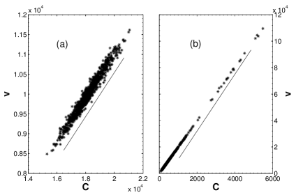
Figure 1: Number of visitations $V$ vs $C$ in (a) Erdős-Rényi networks with $N=1000$ nodes and the connecting probability $p=0.36$ and (b) scale-free networks generated by the Barabási-Albert algorithm, with $N=1000$ nodes, and an average degree of $6$. We assign a random value $w_{ij}$, which is randomly chosen from [1,100], to each $t_{ij}$. We originally set $M=5$ and $N_{s}=10^{10}$ to ensure the system reach the equilibrium phase. The simulations have at least $10^{3}$ realizations.

Also, this approach can be easily applied to more general cases, in which nodes are linked with unequal weight $\{w_{ij}\}$. To deal with those cases, we multiply each link $A_{ij}$ by $w_{ij}$ and then replace degree $K_{i}$ by $C_{i}=\sum_{l\neq i}w_{il}A_{il}$, a quantity which is similar to fitness defined in Ref. Bianconi , in Eq. (4). With these changes, we can show that one of the ground state of the Hamiltonian is given by

$$\widetilde{\Phi}_{0}=\frac{1}{\sqrt{\sum_{n}C_{n}}}\sum_{i}^{N}\sqrt{C_{i}}|i\rangle$$ (13)

by repeating the above procedure. Therefore, the probability for finding a particle at node $i$ should be equal to

$$p_{i}=\frac{C_{i}}{\sum_{n}C_{n}}$$ (14)

in the infinite time limit.

Our numerical simulation confirms also these results. By displacing randomly $M$ non-interacting particles on random scale-free networks with a specific set of linking amplitudes, we count the number $v_{i}$ of visitations to node $i$ after each particle hops $N$ steps. As shown in Fig. 1(b), indeed, $v_{i}$ is strictly proportional to capacity $C_{i}$ of the node. Furthermore, we find that similar results for ER networks[Fig.1(a)].

Up to now, we have not discussed degeneracy of the ground state yet. In fact, this quantity gives the number of connected components in the network. To make this point more clear, let us first consider a completely connected network. In this case, matrix $H$ in Eq. (5) is irreducible. Furthermore, its off-diagonal elements are either zero or negative unit. Therefore, Perron-Fröbenius theorem in matrix theory applies Franklin . It tells us that the lowest eigenvector of the matrix is unique. In other words, the ground state $\Phi_{0}$ is nondegenerate in this case.

On the other hand, if the network consists of several disjoint components, then Hamiltonian (1) has a nondegenerate ground state on each of them. Moreover, as shown above, the lowest eigenvalue of the Hamiltonian is always zero. Consequently, degeneracy of the ground-state energy $E_{0}=0$ is equal to $N_{c}$, the number of connected components in the network.

To show usefulness of this result, we investigate numerically some widely studied complex network, the so-called Poisson random graph. In this model, the probability for degree $K_{i}$ of node $i$ taking on a specific value $k$ is given by

$$p_{k}=e^{-c}\frac{c^{k}}{k!},$$ (15)

where $c>0$ is the distribution mean. In particular, we consider an ensemble of graphs. Each of them has $n$ nodes and $m$ edges and appears with equal probability. In the following, we denote this ensemble by $G_{n,m}$.

Our data are shown in Fig. 2. We find that, for $m\leq n/2$, degeneracy of the ground-state is roughly equal to $D=n-m$. However, when $z=2m/n>1$, $D$ decreases non-linearly as $m$ further increases. This change of behavior around $z=1$ can be clearly seen by taking the first order derivative of the fitting curves. It suggests that a dynamic phase transition may occur at point $z=1$. Our findings are consistent with the previous graph theoretic results Bollobas .

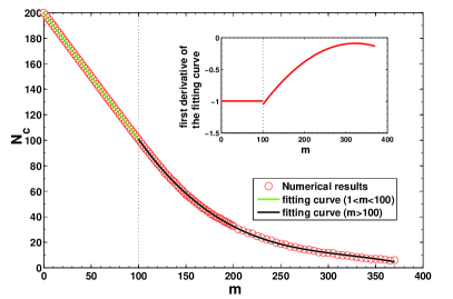
Figure 2: The number of components in random graphs with $n$ vertices and $m$ edges. Each point is an average over $10^{3}$ networks of $200$ vertices each.

In addition, we observe also that the first excited state of Hamiltonian (1) is generally nondegenerate in our simulations. Moreover, its wave function is actually located on the the largest connected component of the network. In other words, the coefficients $b_{i}$’s in the expansion of the first excited wave function

$$\Phi_{1}=\sum_{i}b_{i}|i\rangle$$ (16)

are only nonzero for those nodes which belong to the same connected subset of the largest size. Our data are shown in Fig. 3. From it, one can easily see that, as $m$ varies, the number of nonzero expansion coefficients in $\Phi_{1}$ is always equal to the size of the largest connected component, which is figured out by the standard depth-first search traversing algorithm. Moreover, there always exists a single largest connected component in each realization of network.

From quantum mechanical point of view, this observation is not difficult to understand. Let us think of each connected component of the network as a three-dimensional infinitely deep potential well. Then, as is well known in quantum mechanics, the energy gap between the first excited state and the ground state of Hamiltonian (1) in each well is proportional to $V^{-2/3}$, where $V$ is volume of the well Landau . In other words, the gap decreases as the number of nodes in the connected component becomes larger. Consequently, one will expect that the smallest energy gap is reached in the largest well (connected component). On the other hand, we have shown above that all the ground state energies on the connected components of network are fixed at $E_{0}=0$. Therefore, the global first excited state must appear in the largest connected component.

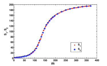
Figure 3: The largest component size $S_{1}$ and the number of $\Phi_{1}$’s nonzero expansion coefficients $S_{2}$ in ER random networks with $n=200$ vertices and $m$ edges. Red points indicate the number of nonzero expansion coefficients in $\Phi_{1}$, while blue points are the results of the depth-first search traversing algorithm on the same network. Each point is an average over $10^{3}$ networks of $200$ vertices each.

Furthermore, we conjecture that the higher excited energy spectrum of this model can be used to reveal other characters of networks, such as modularity. We shall address this issue in future investigation.

In summary, we introduce a non-interacting boson model on complex networks to investigate their structures in the present paper. Our motivation is based on the following observation: It is the structure of a specific network that determines the flow of particles in it. Therefore, our knowledge on particle dynamics should be conversely useful to uncover topology of the network. Indeed, we show that the ground state energy of this model is degenerate if the network consists of $N_{c}$ disjoint connected components and its degeneracy coincides with $N_{c}$. Moreover, the square of each coefficient in the expansion of ground state gives the correct averaged time for a random walker spending at a specific node $i$ in the infinite time limit. Finally, we show also that the first excited state of the model is always supported on the largest connected component of network. Therefore, it gives us a practical way to detect topological structures of complex networks.

This work is partially supported by the National Basic Research Program of China (Grant No. 2005CB321900). One of us (G. S. T) is also supported by the Chinese National Science Foundation under Grant No. 10674003 and MOST grant 2006CB921300.

References

- (1) R. Albert and A.-L.Barabási, Rev. Mod. Phys. 74, 47 (2002).
- (2) M. E. J. Newman, SIAM Rev. 45, 167 (2003).
- (3) S. N. Dorogovtsev, A. V. Goltsev, and J. F. Mendes, Rev. Mod. Phys. 80, 1275 (2008).
- (4) W. Leland, M. Taqqu, W. Willinger, and D. Wilson, IEEE/ACM Transactions on Networking (TON). 2, 1 (1994).
- (5) A virtual round table on ten leading questions for network research can be found in the special issue on Applications of Networks, edited by G. Caldarelli, A. Erzan, and A. Vespignani [Eur. Phys. J. B 38, 143 (2004)].
- (6) J. D. Noh and H. Rieger, Phys. Rev. Lett. 92, 118701 (2004).
- (7) B. Danila, Y. Yu, S. Earl, J. A. Marsh, Z. Toroczkai, and K. E. Bassler, Phys. Rev. E 74, 046114 (2006).
- (8) W.-X. Wang, B.-H. Wang, C.-Y. Yin, Y.-B. Xie, and T. Zhou, Phys. Rev. E 73, 026111 (2006).
- (9) D. Stauffer and M. Sahimi, Phys. Rev. E 72, 046128 (2005).
- (10) A. Baronchelli, M. Catanzaro, and R. Pastor-Satorras, Phys. Rev. E 78, 011114 (2008).
- (11) J. D. Noh, H. Lee, and G. M. Shim, Phys. Rev. Lett. 94, 198701 (2005).
- (12) M. Maragakis, S. Carmi, D. ben-Avraham, S. Havlin, and P. Argyrakis, Phys. Rev. E 77, 020103 (2008).
- (13) M. R. Evans, T. Hanney, and S. N. Majumdar, Phys. Rev. Lett. 97, 010602 (2006).
- (14) E. Lopez, S. V. Buldyrev, S. Havlin, and H. E. Stanley, Phys. Rev. Lett. 94, 248701 (2005).
- (15) M. Crovella and A. Bestavros, IEEE/ACM Transactions on Networking (TON) 5, 835 (1997).
- (16) A. P. S. de Moura, Phys. Rev. E 71, 066114 (2005).
- (17) R. Germano and A. P. S. de Moura, Phys. Rev. E 74, 036117 (2006).
- (18) D. S. Callaway, M. E. J. Newman, S. H. Strogatz, and D. J. Watts, Phys. Rev. Lett. 85, 5468 (2000).
- (19) R. Pastor-Satorras and A. Vespignani, Phys. Rev. Lett. 86, 3200 (2001); Phys. Rev. E 65 035108 (2002).
- (20) D. J. Watts, P. S. Dodds, and M. E. J. Newman, Science 296, 1302 (2002).
- (21) A. V. Goltsev, S. N. Dorogovtsev, and J. F. Mendes, Phys. Rev. E 78, 051105 (2008).
- (22) B. Bollobás, Modern Graph Theory (Springer-Verlag, New York, 1998).
- (23) L. Jahnke, J. W. Kantelhardt, R. Berkovits, and S. Havlin, Phys. Rev. Lett. 101, 175702 (2008).
- (24) J. Franklin, Matrix Theory (Prentice Hall, Englewood Cliffs, New Jersey, 1968).
- (25) G. Bianconi and A.-L. Barabási, Phys. Rev. Lett. 86, 5632 (2001).
- (26) L. D. Landau and E. M. Lifshitz, Statistical Physics (Pergamon Press, Oxford, 1980), p. 14.