DIFFERENTIAL CROSS SECTION OF DP-ELASTIC SCATTERING AT INTERMEDIATE ENERGIES

Abstract

The deuteron-proton elastic scattering is studied in the multiple scattering expansion formalism. The contributions of the one-nucleon-exchange, single- and double scattering are taken into account. The Love and Franey parameterization of the nucleon-nucleon $t$-matrix is used, that gives an opportunity to include the off-energy-shell effects into calculations. Differential cross sections are considered at four energies, $T_{d}=390,500,880,1200$ MeV. The obtained results are compared with the experimental data.

1 Introduction

The study of the deuteron-proton elastic scattering has a longtime story. The first nucleon-deuteron experiments were performed already in fifties of the previous century scham -postma . Differential cross sections scham -crewe and polarization marshal -postma were measured at few hundred MeV. Nowadays this reaction is still the subject of investigations cr500 -pkur . This process is the simplest example of the hadron nucleus collision that is why the interest to this reaction is justified. A number of experiments on deuteron- nucleon elastic scattering is aimed at getting some information about the deuteron wave function and nucleon-nucleon amplitudes from $Nd$ scattering observables. Moreover, the study of the reaction mechanisms, investigations of the few-body scattering dynamics are also very important to understand the nature of nuclear interactions.

A good theoretical description of the deuteron-nucleon process was obtained for low energies, where the multiple scattering formalism based on the solution of the Faddeev equations, has been applied to solve this problem glrew . However, at the energies above 150 MeV there is some discrepancy between the experimental data and theoretical predictions in the minimum of the differential cross section. At present many efforts are undertaken to extend the Faddeev calculation technique into the relativistic regime elster72 -elster78 . But up to now there are no reasonable descriptions of the experimental data obtained in the Faddeev equation framework at intermediate energies.

Also p-d scattering at low energies was considered in the approach based on the solution of the three-particle Schrödinger equation using the Kohn variational principle (KVP)kiev30 ,deltuva65 . Special attention in these works was given to the study of the Coulomb effects. It has been shown that at the energies below 30 MeV the influence of the Coulomb interaction is appreciable, while it considerably reduces at $T_{lab}=65$ MeV deltuva65 .

The high-energy deuteron-proton scattering in the forward hemisphere is successfully described by the Glauber theory which takes both single and double interactions into account franco ,francol . In har it is shown that filling of the minimum, due to the interference between the single- and double-scattering amplitudes, is explained by the presence of the D-wave in the deuteron wave function.

However, as it is shown in alberi , japh , the off-energy-shell effects begin to play an important role at scattering angles larger than $30^{0}$ in c.m. In kaptari the deuteron-proton backward elastic scattering was considered in the Bethe-Salpeter approach. Here various relativistic effects were studied. It has been shown, that the relativistic corrections coming from the negative energy P-waves are negligible while Lorentz boost effects become evident already at $P_{lab}\sim 0.2\div 0.3$ GeV/c (here,$P_{lab}$ is the scattered proton momentum in the laboratory frame).

The present paper considers the intermediate energy range from 200 MeV up to 600 MeV of the initial nucleon. On the one hand, the energies are not large enough to apply the Glauber theory. On the other hand, in this region it is already necessary to take relativistic effects into account and as a consequence the Faddeev calculation technique does not work properly at these energies. Nevertheless, at these energies it is still possible to use a non-relativistic deuteron wave function due to transfer into the deuteron Breit frame. Here, it is also very important to describe correctly the nucleon- nucleon vertices, namely the spin structure as well as angular and energy dependences.

In the previous paper japh the polarization observables, such as vector and tensor analyzing powers, were studied in the presented approach. In this work only the differential cross sections are considered at four energies. The energy range has been chosen to demonstrate the region, where this model is justified.

Sect.2 gives the expression for the differential cross section and general kinematical definitions. The theoretical formalism is presented in Sect.3. We consider a multiply-scattering series up to the second-order terms of the nucleon-nucleon $t$-matrix. The iterations of the Alt-Grassberger-Sandhas equations is performed to get this expansion. The wave function of the moving deuteron, which depends on the two variables, is used in the calculations.

We apply the $NN$ $t$-matrix constructed by Love and Franey LF in order to describe the nucleon-nucleon interactions. This parameterization allows one to take the energy and angular dependences into account. Moreover, it is possible to extend this approach to the off-energy-shell region. The results of the calculations are discussed in Sect.4. The conclusions are given in Sect.5.

2 Kinematics

A cross section of the $dp$-scattering is expressed via the squared reaction amplitude:

$$\sigma(dp\to dp)=(2\pi)^{4}\frac{1}{6}\int\frac{d\vec{P}_{d}^{\prime}}{E_{d}^{\prime}}\frac{d\vec{p}_{p}^{\prime}}{E_{p}^{\prime}}\delta(E_{d}+E_{p}-E_{d}^{\prime}-E_{p}^{\prime})$$

$$\delta(\vec{P}_{d}+\vec{p}-\vec{P}_{d}^{\prime}-\vec{p}^{\prime})\frac{|\sqrt{E_{d}^{\prime}E_{p}^{\prime}}~{}~{}{\cal J}\sqrt{E_{d}E_{p}}|^{2}}{\sqrt{(P_{d}p)^{2}-P_{d}^{2}p^{2}}}.$$ (1)

This expression is valid for an arbitrary frame. Here $(E_{d},P_{d})$, $(E_{p},p)$ are the energies and momenta of the initial deuteron and proton, respectively. The corresponding variables for the final particles are defined with the primed symbols. Starting from Eq.(2) one can obtain a formula for the differential cross section in the center-of-mass,

$$\frac{d\sigma}{d\Omega^{*}}=(2\pi)^{4}\cdot\frac{1}{6}\cdot\frac{1}{s}|\sqrt{E_{d}^{\prime}E_{p}^{\prime}}~{}~{}{\cal J}\sqrt{E_{d}E_{p}}|^{2}.$$ (2)

It should be emphasized that expression
$|\sqrt{E_{d}^{\prime}E_{p}^{\prime}}~{}~{}{\cal J}\sqrt{E_{d}E_{p}}|^{2}$ is invariant. Since the reaction amplitude ${\cal J}$ is calculated in the Breit frame, the energies should be also defined in the same system:

$$E_{d} = E_{d}^{\prime}=\sqrt{M_{d}^{2}+\vec{Q}^{2}},~{}~{}~{}\vec{Q}^{2}=-t/4,~{}~{}~{}$$ (3)

$$E_{p} = E_{p}^{\prime}=\sqrt{m_{N}^{2}+\vec{p}^{2}},~{}~{}~{}~{}(\vec{p}\vec{Q})=-\vec{Q}^{2},$$ (4)

where $M_{d}$ and $m_{N}$ correspond to the deuteron and nucleon masses, respectively, and $\vec{Q}$, $\vec{p}$ are momenta of the deuteron and proton in the Breit frame. The Mandelstam variables $s$ and $t$ are defined through the laboratory deuteron energy and center-of-mass angle, $\theta^{*}$,

$$s = (P_{d}+p)^{2}=M_{d}^{2}+m_{N}^{2}+2m_{N}E_{d}^{lab}$$

$$t = (P_{d}-P_{d}^{\prime})^{2}=-\frac{4m_{N}^{2}}{s}(\vec{P}_{d}^{lab})^{2}(1-\cos\theta^{*}).$$ (5)

3 General formalism

According to the three-body collision theory, the amplitude of the deuteron-proton elastic scattering $\cal J$ is defined by the matrix element of the transition operator $U_{11}$:

$$U_{dp\to dp} = \delta(E_{d}+E_{p}-E^{\prime}_{d}-E^{\prime}_{p}){\cal J}=$$ (6)

$$<1(23)|[1-P_{12}-P_{13}]U_{11}|1(23)>.$$

Here, the state $|1(23)>$ corresponds to the configuration, when nucleons 2 and 3 form the deuteron state and nucleon 1 is free. Emergence of the permutation operators for two nucleons $P_{ij}$ reflects the fact that the initial and final states are antisymmetric due to the two particles exchange.

The transition operators for rearrangement scattering are defined by the Alt–Grassberger–Sandhas equations Alt –AGS :

$$U_{11} = ~{}~{}~{}~{}~{}~{}~{}~{}t_{2}g_{0}U_{21}+t_{3}g_{0}U_{31},$$

$$U_{21} = g_{0}^{-1}+t_{1}g_{0}U_{11}+t_{3}g_{0}U_{31},$$ (7)

$$U_{31} = g_{0}^{-1}+t_{1}g_{0}U_{11}+t_{2}g_{0}U_{21},$$

where $t_{1}=t(2,3)$, etc., is the $t$-matrix of the two-nucleon interaction and $g_{0}$ is the free three-particle propagator. The indices $ij$ for the transition operators $U_{ij}$ denote free particles $i$ and $j$ in the final and initial states, respectively.

Iterating these equations up to the $t_{i}$-second-order terms, we can present the reaction amplitude as a sum of the following three contributions: one-nucleon exchange, single scattering, and double scattering:

$${\cal J}_{dp\to dp} = {\cal J}_{\rm ONE}+{\cal J}_{\rm SS}+{\cal J}_{\rm DS},$$

$${\cal J}_{\rm ONE} = -2<1(23)|P_{12}g_{0}^{-1}|1(23)>,$$

$${\cal J}_{\rm SS} = 2<1(23)|t_{3}^{\rm sym}|1(23)>,$$ (8)

$${\cal J}_{\rm DS} = 2<1(23)|t_{3}^{\rm sym}g_{0}t_{2}^{\rm sym}|1(23)>,$$

where we have introduced notations for antisymmetrized operators $t_{2}^{\rm sym}=[1-P_{13}]t_{2}$ and $t_{3}^{\rm sym}=[1-P_{12}]t_{3}$. Schematically, this sequence is shown in Fig.1.

The convergence of the multiple scattering series was studied in ref.witala ,elster78 . A reasonable agreement between the results of the calculations taking the second order corrections into account and the full Faddeev calculations, was obtained at the laboratory energies up to 2 GeV at least for the forward scattering angles. The analogous conclusion can be done for the differential cross section of the elastic scattering at $E_{lab}=400$ MeV for the scattering angle up to $140^{0}$ witala . It gives us the ground to suppose that the reduced series (3) is a good approximation to describe dp-elastic scattering at the energies above 400 MeV.

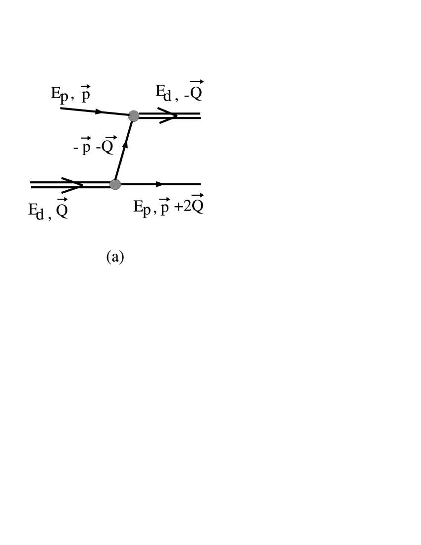
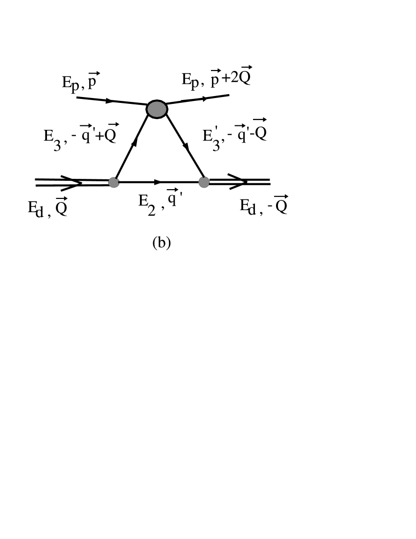
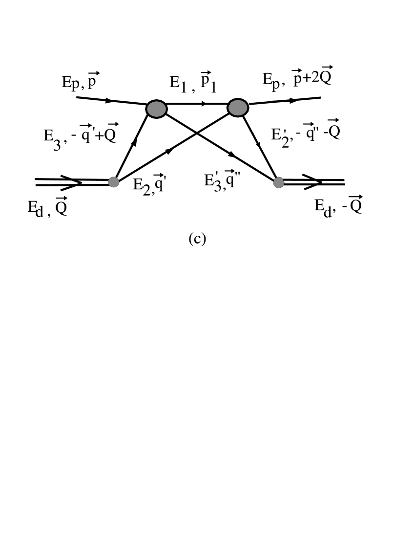
Figure 1: The diagrams are taken into consideration: one-nucleon-exchange (a), single scattering (b), and double scattering (c) graphs.

After straightforward calculations we have got the following expressions:
for the one-nucleon-exchange amplitude –

$${\cal J}_{ONE} = -\frac{1}{2}(E_{d}-E_{p}-\sqrt{m_{N}^{2}+\vec{p}~{}^{2}-\vec{Q}\-^{2}})\cdot$$

$$<\vec{p}^{\prime}\mu^{\prime};-\vec{Q}{\cal M}_{d}^{\prime}|\Omega^{\dagger}_{d}(23)[1+(\mbox{\boldmath$\sigma_{1}\sigma_{2}$})]\Omega_{d}(23)|\vec{Q}{\cal M}_{d};\vec{p}\mu>~{}~{},$$

for the single scattering amplitude –

$${\cal J}_{SS} = \int d\vec{q}~{}^{\prime}<-\vec{Q}{\cal M}_{d}^{\prime}|\Omega_{d}^{\dagger}|\vec{q}~{}^{\prime}\mu_{2},-\vec{Q}-\vec{q}~{}^{\prime}\mu_{3}^{\prime}>$$

$$<\vec{p}~{}^{\prime}\mu^{\prime},-\vec{Q}-\vec{q}~{}^{\prime}\mu_{3}^{\prime}|\frac{3}{2}t^{1}_{13}(E)+\frac{1}{2}t^{0}_{13}(E)|\vec{p}\mu,\vec{Q}-\vec{q}~{}^{\prime}\mu_{3}>$$

$$<\vec{q}~{}^{\prime}\mu_{2},\vec{Q}-\vec{q}~{}^{\prime}\mu_{3}|\Omega_{d}|\vec{Q}{\cal M}_{d}>~{}~{}.$$

for the double scattering amplitude –

$${\cal J}_{DS}=\int d\vec{q}~{}^{\prime}\int d\vec{q}^{\prime\prime}<-\vec{Q}{\cal M}_{d}^{\prime}|\Omega_{d}^{\dagger}$$ (11)

$$|-\vec{Q}-\vec{q}~{}^{\prime\prime}~{}\mu_{2}^{\prime},\vec{q}~{}^{\prime\prime}~{}\mu_{3}^{\prime}><\vec{p}^{\prime}~{}\mu^{\prime},-\vec{Q}-\vec{q}~{}^{\prime\prime}~{}\mu_{2}^{\prime},\vec{q}~{}^{\prime\prime}~{}\mu_{3}^{\prime}|$$

$$\frac{t_{12}^{1}(E^{\prime})t_{13}^{1}(E)+[t_{12}^{1}(E^{\prime})+t_{12}^{0}(E^{\prime})][t_{13}^{1}(E)+t_{13}^{0}(E)]/4}{E_{d}+E_{p}-E_{1}-E_{2}-E_{3}^{\prime}+i\varepsilon}$$

$$|\vec{p}~{}\mu,\vec{q}~{}^{\prime}~{}\mu_{2},\vec{Q}-\vec{q}~{}^{\prime}~{}\mu_{3}>$$

$$<\vec{q}~{}^{\prime}~{}\mu_{2},~{}\vec{Q}-\vec{q}~{}^{\prime}~{}\mu_{3}|\Omega_{d}|\vec{Q}{\cal M}_{d}>.$$

Here the spin projections are denoted as $\mu$ for nucleons and ${\cal M}_{d}$ – for deuterons. Henceforth, all summations over dummy discrete indices are implied. The superscript of the $t$-matrix corresponds to the isotopic spin of the nucleon-nucleon state. The argument of the $NN$-matrix is defined as the three-nucleon on-shell energy excluding the energy of the nucleon which does not participate in the interaction:

$$E=E_{d}+E_{p}-E_{2},~{}~{}~{}~{}~{}~{}E^{\prime}=E_{d}+E_{p}-E^{\prime}_{3}.$$ (12)

The three-nucleon free propagator in Eq.(11) can be decomposed on two terms using the well-known formula:

$$\frac{1}{E_{d}+E_{p}-E_{1}-E_{2}-E_{3}^{\prime}+i\varepsilon}=$$ (13)

$${\cal P}\frac{1}{E_{d}+E_{p}-E_{1}-E_{2}-E_{3}^{\prime}}$$

$$-i\pi\delta(E_{d}+E_{p}-E_{1}-E_{2}-E_{3}^{\prime}).$$

The principal value part is often neglected to simplify the further calculations. However, as it was shown in japh , it is very important to take into account the full representation of the three-nucleon propagator, especially, at the scattering angles above $40^{0}$.

All the calculations are performed in the deuteron Breit frame, where the deuterons move in opposite directions with equal momenta (Fig.1). It allows us to minimize the relative momenta of the nucleons in the both deuterons. As a consequence, the non-relativistic deuteron wave function can be applied in the energy range under consideration.

In the rest frame the non-relativistic wave function of the deuteron depends only on one variable $\vec{p}_{0}$, which is the relative momentum of the outgoing proton and neutron:

$$<\mu_{p}\mu_{n}|\Omega_{d}|{\cal M}_{d}>=\frac{1}{\sqrt{4\pi}}<\mu_{p}\mu_{n}|\{u(p_{0})+$$ (14)

$$\hskip 56.9055pt\frac{w(p_{0})}{\sqrt{8}}[3(\mbox{\boldmath$\sigma_{1}$}\hat{p}_{0})(\mbox{\boldmath$\sigma_{2}$}\hat{p}_{0})-(\mbox{\boldmath$\sigma_{1}$ $\sigma_{2}$})]\}|{\cal M}_{d}>,$$

where $u(p_{0})$ and $w(p_{0})$ describe the $S$ and $D$ components of the deuteron wave function B , cd , par , $\hat{p}_{0}$ is the unit vector in $\vec{p}_{0}$ direction.

In order to get the wave function of the moving deuteron, it is necessary to apply the Lorenz transformations for the kinematical variables and Wigner rotations for the spin states. This procedure has been expounded in japh , and, here, we give only the result:

$$<\vec{p}_{1}~{}\mu_{1},\vec{p}_{2}\mu_{2}|\Omega_{d}|\vec{Q},{\cal M}_{d}>=<\vec{p}_{1}~{}\mu_{1},\vec{p}_{2}\mu_{2}|g_{1}(\vec{k},\vec{Q})+$$

$$g_{2}(\vec{k},\vec{Q})(\mbox{\boldmath$\sigma_{1}$}\vec{n})(\mbox{\boldmath$\sigma_{2}$}\vec{n})+g_{3}(\vec{k},\vec{Q})(\mbox{\boldmath$\sigma_{1}\sigma_{2}$})+$$

$$+ g_{4}(\vec{k},\vec{Q})(\mbox{\boldmath$\sigma_{1}$}\hat{k})(\mbox{\boldmath$\sigma_{2}$}\hat{k})+g_{5}(\vec{k},\vec{Q})((\mbox{\boldmath$\sigma_{1}$}+\mbox{\boldmath$\sigma_{2}$})\vec{n})+$$

$$+ g_{6}(\vec{k},\vec{Q})[(\mbox{\boldmath$\sigma_{1}$}\hat{k})(\mbox{\boldmath$\sigma_{2}$},\vec{n}\times\hat{k})+(\mbox{\boldmath$\sigma_{1}$},\vec{n}\times\hat{k})(\mbox{\boldmath$\sigma_{2}$}\hat{k})]|\vec{Q},{\cal M}_{d}>.$$

Note, the wave function of the moving deuteron is the function of two variables: the deuteron momentum $\vec{Q}$ and neutron-proton relative momentum $\vec{k}$ –

$$\vec{Q}=\vec{p}_{1}+\vec{p}_{2},$$

$$\vec{k}=\frac{(E_{2}+\sqrt{s}/2)\vec{p}_{1}-(E_{1}+\sqrt{s}/2)\vec{p}_{2}}{E_{1}+E_{2}+\sqrt{s}}.$$ (16)

Here $(E_{1},\vec{p}_{1})$ and $(E_{2},\vec{p}_{2})$ are the energy and momentum of the neutron and proton in the deuteron, and $s$ is the squared sum of the neutron and proton 4-momenta, $s=(p_{1}+p_{2})^{2}$. The normal to $(\vec{p}_{1},\vec{p}_{2})$-plane is denoted as $\vec{n}$.

In general, functions $g_{i}$ can be obtained by solving a relativistic equation, as it was done in karmanov1 –carbonell in the light front model. But in the present paper a usual non-relativistic DWF is taken as an input. Therefore, functions $g_{i}$ are defined as the linear combinations of $u$ and $w$ ($S$- and $D$-waves).

In order to describe the nucleon- nucleon interaction in a wide energy region, we have used the Love and Franey parameterization LF of the $NN$ $t$-matrix defined in the center-of-mass as

$$<\mbox{\boldmath$\kappa$}^{\prime}\mu_{1}^{\prime}\mu_{2}^{\prime}|t_{c.m.}|\mbox{\boldmath$\kappa$}\mu_{1}\mu_{2}>=<\mbox{\boldmath$\kappa$}^{\prime}\mu_{1}^{\prime}\mu_{2}^{\prime}|A+$$ (17)

$$B(\mbox{\boldmath$\sigma_{1}$}\hat{N}^{*})(\mbox{\boldmath$\sigma_{2}$}\hat{N}^{*})+C(\mbox{\boldmath$\sigma_{1}$}+\mbox{\boldmath$\sigma_{2}$})\cdot\hat{N}^{*}+D(\mbox{\boldmath$\sigma_{1}$}\hat{q}^{*})(\mbox{\boldmath$\sigma_{2}$}\hat{q}^{*})+$$

$$F(\mbox{\boldmath$\sigma_{1}$}\hat{Q}^{*})(\mbox{\boldmath$\sigma_{2}$}\hat{Q}^{*})|\mbox{\boldmath$\kappa$}\mu_{1}\mu_{2}>.$$

Here the orthonormal basis is combinations of the nucleons’ relative momenta in the initial $\kappa$ and final $\kappa$^′ states:

$$\hat{q}^{*}=\frac{\mbox{\boldmath$\kappa$}-\mbox{\boldmath$\kappa$}^{\prime}}{|\mbox{\boldmath$\kappa$}-\mbox{\boldmath$\kappa$}^{\prime}|},~{}~{}\hat{Q}^{*}=\frac{\mbox{\boldmath$\kappa$}+\mbox{\boldmath$\kappa$}^{\prime}}{|\mbox{\boldmath$\kappa$}+\mbox{\boldmath$\kappa$}^{\prime}|},~{}~{}\hat{N}^{*}=\frac{\mbox{\boldmath$\kappa$}\times\mbox{\boldmath$\kappa$}^{\prime}}{|\mbox{\boldmath$\kappa$}\times\mbox{\boldmath$\kappa$}^{\prime}|}.$$ (18)

The amplitudes $A,B,C,D,F$ are the functions from the center-of-mass energy and scattering angle. The radial parts of these amplitudes are taken as a sum of Yukawa terms. A new fit of the model parameters was done newlf according to the current phase-shift-analysis data SP07 said .

Since the matrix elements are expressed through the effective $NN$-interaction operators sandwiched between the initial and final plane-wave states, this construction can be extended to the off-shell case allowing the initial and final states to get the current values of the $\kappa$ and $\kappa^{\prime}$. Obviously, this extrapolation does not change the general spin structure.

To use definition (17) for the nucleon-nucleon matrix in the further calculation, it is necessary to relate $t$-matrices in the two-nucleons c.m. and in the deuteron Breit frame. This relation can be obtained by using the Lorenz transformation and Wigner rotation technique as it was done for the deuteron wave function. This problem has been considered in detail in fbs , japh .

$$<\vec{p}^{\prime}\vec{p}_{3}^{\prime};\mu^{\prime}\mu_{3}^{\prime}|t(E)|\vec{p}\vec{p}_{3};\mu\mu_{3}>={\cal NF}<\kappa^{\prime}\mu_{1}^{\prime}\mu_{2}^{\prime}|$$

$$W^{\dagger}_{1/2}(\vec{p}^{\prime})W^{\dagger}_{1/2}(\vec{p}_{3}^{\prime})t_{c.m.}(\sqrt{s})~{}W_{1/2}(\vec{p})W_{1/2}(\vec{p}_{3})|\kappa\mu_{1}\mu_{2}>.$$

Here, momentum notations correspond to the ones given in Fig.1b. The Wigner rotations of the initial and final states are performed around $\vec{n}$ and $\vec{n}^{\prime}$ axes, respectively:

$$\vec{n}=\frac{\vec{p}\times\vec{p}_{3}}{|\vec{p}\times\vec{p}_{3}|},~{}~{}~{}~{}~{}~{}~{}~{}\vec{n}^{\prime}=\frac{\vec{p}~{}^{\prime}\times\vec{p}_{3}~{}^{\prime}}{|\vec{p}~{}^{\prime}\times\vec{p}_{3}~{}^{\prime}|}.$$ (20)

The Wigner rotation operator in the spin space of the $i$-th nucleon has the standard form:

$$W_{1/2}(\vec{p}_{i},\vec{u})={\rm exp}\left\{-i\omega_{i}(\vec{n}_{i}\mbox{\boldmath$\sigma_{i}$})/2\right\}=$$ (21)

$${\rm cos}(\omega_{i}/2)[1-i(\vec{n}_{i}\mbox{\boldmath$\sigma_{i}$}){\rm tg}(\omega_{i}/2)],$$

where $\omega_{i}$ is the angle of this rotation. The normalization factor ${\cal N}$ provides conditions of orthonormality and completeness and is defined by the Jacobian of the transformations. The kinematical factor ${\cal F}$ is due to the relation between two off-energy shell $t$-matrices, one of them depends on zero total momentum garcilazo , japh .

The argument of the $t$-matrix in the right-hand side of Eq.(3) is the square root of the Mandelstam variable $s$, which is defined through the kinematical variables in the deuteron Breit frame taken on the mass-shell:

$$s=E^{2}-\vec{K}^{2},$$ (22)

where $\vec{K}=\vec{p}+\vec{p}_{3}$ is the total momentum of the nucleon-nucleon pair in the frame of the calculation.

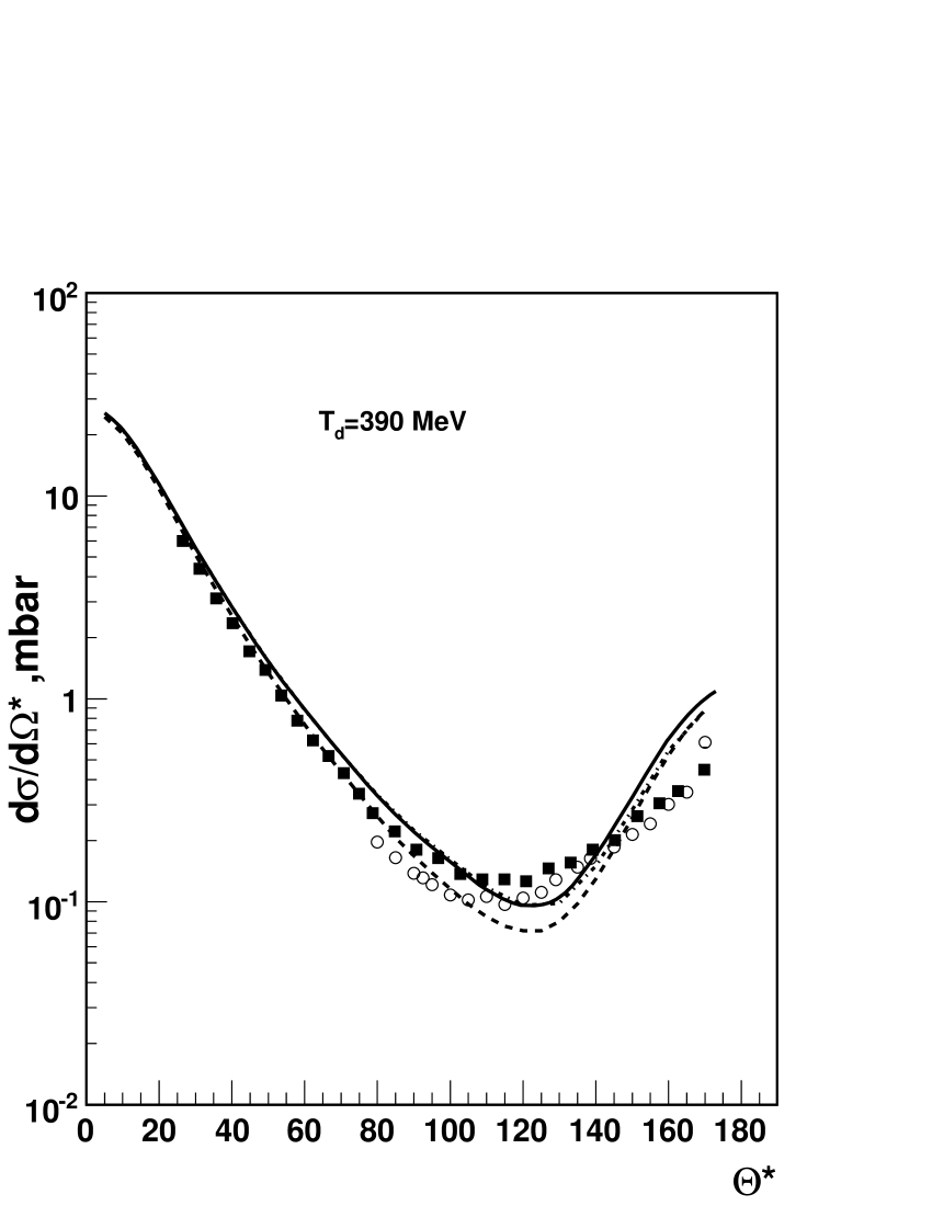
Figure 2: The differential cross section at the deuteron kinetic energy of 390 MeV as a function of the c.m. scattering angle. The dashed line corresponds to the calculations including only one-nucleon-exchange and single scattering diagrams into consideration. The solid and dashed-dotted lines are the results of the calculations taking into account also the double scattering diagram with the principal value part of the free propagator and without it, respectively. The data are taken from ermish ($\blacksquare$) and adelberger ($\bigcirc$).

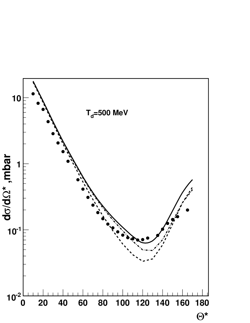
Figure 3: The differential cross section at the deuteron kinetic energy of 500 MeV as a function of the c.m. scattering angle. The lines are the same as in Fig.2. The data are taken fromcr500 .

4 Results and discussion

The results of the calculations for the differential cross sections are presented in Figs.2-5. The four deuteron kinetic energies, 390, 500, 880 and 1200 MeV, have been considered. All calculations were performed with the CD-Bonn deuteron wave function cd . The dashed line in Figs.2-5 corresponds to the calculations taking into account only ONE and single-scattering contributions. The dash-dotted line represents the calculation including the double-scattering term without the principal value part in the three-nucleon propagator, and the solid line stands for the calculations with the full three-nucleon propagator.

One can see that the results taking the double scattering into account and without it, are close to each other up to 50-60 degrees of the scattering angle for all the considered energies. At these angles the single-scattering gives the main contribution to the differential cross section. Then the difference between these results increases. It should be noted that the double scattering contribution is not large enough for the deuteron energy of 390 MeV (Fig.2). As a consequence, the curves corresponding to the results with and without the principal value part of the three-nucleon propagator, are practically undistinguished. However, the double-scattering effect increases with the energy. Already for the energy of 500 MeV (Fig.3) the difference between the results taking DS into consideration and without it, is significant – it is about 2 times in minimum of the differential cross section. For higher energies this factor is even larger: it is about 10 times for $T_{d}=880$ MeV (Fig.4), and about 20 times for the energy equal to 1200 MeV (Fig.5).

The difference between the results taking into account the principal value part of the three-nucleon propagator (”full” calculation) and without it, also increases with the energy. At small angles this deviation is practically invisible, while it is significant for the scattering in the backward hemisphere, $\theta^{*}\geq 90^{0}$, where the double scattering effect plays the main role. Such a discrepancy can be, probably, explained by the relativistic effects related with the off-energy-shell behaviour of the nucleon-nucleon $t$-matrices, and Fermi motion of the nucleons in the deuterons. It is interesting to emphasize that the curves corresponding to the calculations without the principal value part of the free propagator are close to the ONE+SS-results at the scattering angle above $160^{0}$ at all the energies under consideration.

The deviation of the theoretical predictions from the experimental data are observed at the scattering angles above $140^{0}$. One can assume some reasons of this distinction. It is possible that the multiple scattering series is not yet converged in the backward direction, and it is necessary to take the more orders of this series into account. This is supposed according to the results of the investigation performed in ref.witala .

The agreement between the experimental data and theoretical predictions could be also improved, if the three-nucleon forces are included into consideration. In fact, a good description of the differential cross sections, both in the diffraction minimum and the backward direction, was obtained at the energies below 400 MeV wit3N , when the three-nucleon forces were taken into account. Unfortunately, at present there are no such calculations at higher energies. However, it should be noted, that the three-nucleon forces can be effectively included through the $\Delta$-isobar excitation. The employment of this approach deltuva gives the results, which are in agreement with the results obtained in wit3N . The essential contribution of the $\Delta$-isobar excitation into the differential cross section was also demonstrated in ref.kapdelta , where the pd-backward elastic scattering was studied at the high energies.

Nevertheless, the results of the ”full” calculations are in a reasonable agreement with the experimental data up to the scattering angle of $140^{0}$ at all the considered energies.

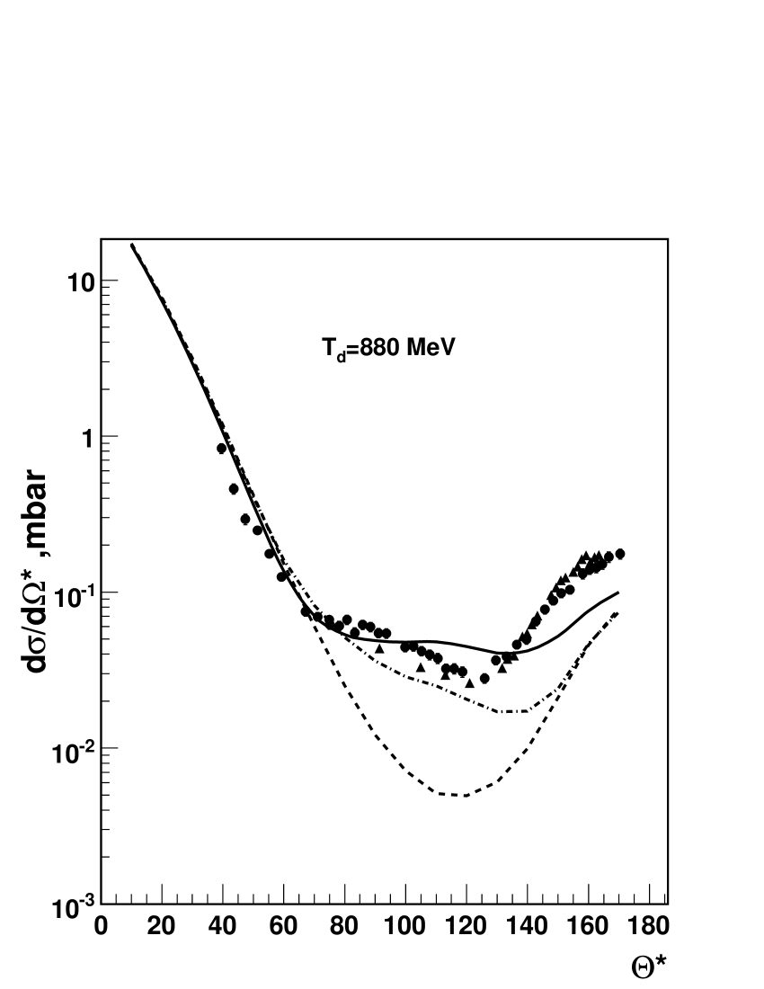
Figure 4: The differential cross section at the deuteron kinetic energy of 880 MeV as a function of the c.m. scattering angle. The lines are the same as in Fig.2. The data are taken from cr880_a ($\bullet$), andcr880_b ($\blacktriangle$).

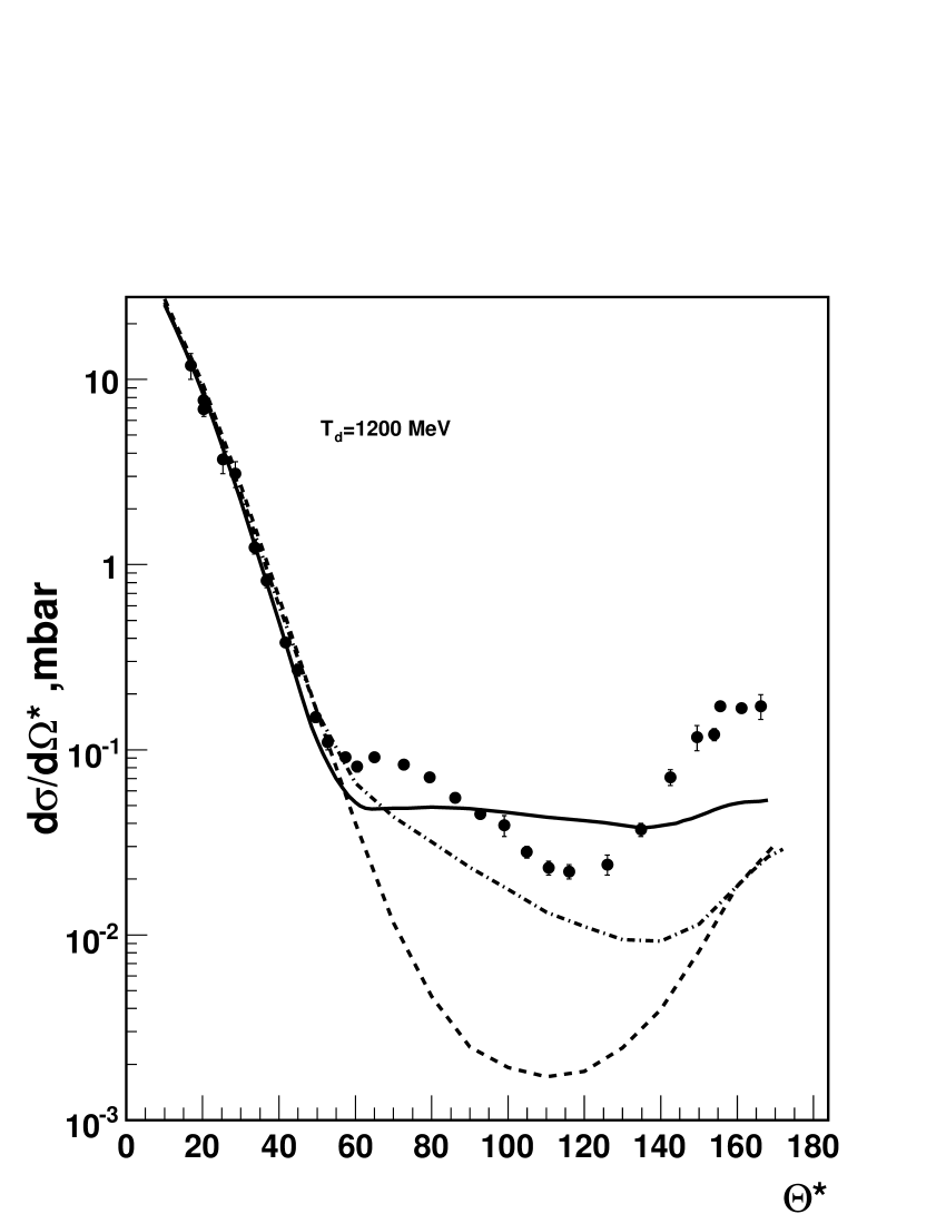
Figure 5: The differential cross section at the deuteron kinetic energy of 1200 MeV as a function of the c.m. scattering angle. The lines are the same as in Fig.2. The data are taken fromcr1200 .

5 Conclusion

In the paper we have presented a method to calculate the amplitude of the deuteron–proton elastic scattering at intermediate energies. Special attention was given to the questions connected with the relativistic effects. The transformation of the deuteron wave function in the rest frame to a moving system was performed, that allowed us to use the non-relativistic DWF at rather high energies. In order to describe nucleon–nucleon interactions in a wide energy range, we have used parameterization of the $NN$ $t$-matrix. The spin transformation technique has been also applied to relate this $t$-matrix given in the c.m. to that in the reference frame.

Using this method we have managed to describe the experimental data on the differential cross section at four energies: 395, 500, 880, and 1200 MeV. Good agreements have been obtained between the experimental data and the theoretical model calculations taking into consideration the one-nucleon-exchange, single- and double-scattering for all the four energies up to the scattering angle of $140^{0}$. The distinctions between the data and theoretical predictions at the backward angles should be studied more precisely, that is the subject for further investigations.

- (1) R.D.Schamberger, Phys.Rev.85, (1952) 424
- (2) O.Chamberlain, M.O.Stern, Phys.Rev.94, (1954) 666
- (3) O.Chamberlain, D.D.Clark, Phys.Rev.102, (1956) 473
- (4) A.V.Crewe, et al., Phys.Rev.114, (1959) 1361
- (5) L.Marshall, et al., Phys.Rev.95, (1954) 1020
- (6) S.Marcowitz, Phys.Rev.120, (1960) 891
- (7) H.Postma, R.Wilson, Phys.Rev.121, (1961) 1229
- (8) K.Hatanaka et al., Phys.Rev.C66, (2002) 044002
- (9) K.Ermish et al., Phys.Rev.C71, (2005) 064004
- (10) P.K.Kurilkin, et al., Eur.Phys.J.St.162, (2008) 137
- (11) W.Glöckle et al., Phys.Rep.274, (1996) 110.
- (12) H.Liu, Ch.Elster, W.Glöckle, Phys.Rev.C72, (2005) 054003
- (13) T.Lin, Ch.Elster, W.N.Polyzou, W.Glöckle, Phys.Rev.C76, (2007) 014010
- (14) T.Lin, et al., Phys.Rev.C78, (2008) 024002
- (15) Ch.Elster, et al, Phys.Rev.C78, (2008) 034002
- (16) A.Kievsky, M.Viviani, S.Rosati, Phys.Rev.C64, (2001) 024002
- (17) A.Deltuva et al., Phys.Rev.C71, (2005) 064003
- (18) V.Franco, Phys.Rev.Lett. 16, (1966) 944
- (19) V.Franco, E.Coleman, Phys.Rev.Lett. 17, (1966) 827
- (20) D.R.Harrington, Phys.Rev.Lett. 21, (1968) 1496
- (21) G.Alberi, M.Bleszynski, T.Jaroszewicz, Ann. Phys.(N.Y.) 142, (1982) 299 .
- (22) N.B.Ladygina, Phys.Atom.Nucl.71,(2008) 2039.
- (23) L.P.Kaptari et al., Phys.Rev. C57, (1998) 1097.
- (24) E.O.Alt, P.Grassberger, W.Sandhas, Nucl.Phys. B2, (1967) 167.
- (25) E.Schmid, H.Ziegelmann,The Quantum Mechanical Three-Body Problem (Oxford, Pergamon Press, 1974).
- (26) R.Machleidt, K.Holinde, Ch.Elster, Phys.Rep. 149, (1987) 1.
- (27) R.Machleidt, Phys. Rev. C63, (2001) 024001.
- (28) M. Lacombe et al., Phys.Lett.B101, (1981) 139.
- (29) V.A.Karmanov, Nucl.Phys.A362, (1981) 331.
- (30) V.A.Karmanov, Phys.Elem. Chast.Atom.Yadra 19, (1988) 525.
- (31) J.Carbonell and V.A.Karmanov, Nucl.Phys.A581, (1995) 625.
- (32) W.G.Love, M.A.Franey, Phys. Rev.C C24, (1981) 1073; W.G.Love, M.A.Franey, Phys.Rev. C 31, (1985) 488.
- (33) N.B.Ladygina, e-preprint nucl-th/0805.3021
- (34) http://gwdac.phys.gwu.edu
- (35) N.B.Ladygina, A.V.Shebeko, Few-Body Syst. 33, (2003) 49.
- (36) H. Garcilazo, Phys.Rev.C16, (1977) 1996.
- (37) R.E.Adelberger, C.N.Brown, Phys.Rev.D5, (1972) 2139.
- (38) N.E.Booth et al., Phys.Rev.D4, (1971) 1261.
- (39) J.C.Alder et al., Phys.Rev.C6, (1972) 2010.
- (40) E.T.Boschitz et al., Phys.Rev.C6, (1972) 457.
- (41) H.Witala et al., Phys.Pev.Lett.81, (1998) 1183.
- (42) A.Deltuva, K.Chmielewski, P.U.Sauer, Phys.Rev.C67, (2003) 034001.
- (43) L.P.Kaptari et al., Few Body Syst.27, (1999) 189.